Standard Analysis for Single-cell scATAC-seq & scRNA-seq Multi-omics: Dimensionality Reduction and Clustering

Author: SeekGene

Time: 8 min

Words: 1.5k words

Updated: 2025-11-20

Reads: 0 times

Overview

Unlike single-omics analysis, dimensionality reduction and clustering for single-cell multi-omics data mainly involves three strategies: RNA-based dimensionality reduction and clustering, ATAC-based dimensionality reduction and clustering, and joint RNA and ATAC integration using Weighted Nearest Neighbors (WNN) dimensionality reduction and clustering.

一. Why Perform Both Separate and Joint Dimensionality Reduction?

The dimensionality reduction strategies for single-cell multi-omics data occur at three levels:

1. RNA-only Dimensionality Reduction and Clustering: Identifies transcriptionally active cell types using gene expression data, reflecting the "functional state" (transcriptional output) of the cell.

2. ATAC-only Dimensionality Reduction and Clustering: Identifies cell types based on chromatin accessibility patterns, reflecting the "regulatory potential" (regulatory state) of the cell.

3. Joint Dimensionality Reduction (WNN): Integrates both RNA and ATAC information sources to construct a weighted nearest neighbor graph, enabling more robust and higher resolution recognition of cell types.

二. Dimensionality Reduction and Clustering on the RNA Modality

1) Data Normalization and Feature Extraction

• SCTransform Normalization: Removes technical factors such as sequencing depth and mitochondrial gene percentage, retaining biological variation.

• Principal Component Analysis (PCA): Reduces the dimensionality of high-dimensional gene expression data to a lower-dimensional space (typically the top 30 principal components), preserving major sources of variation.

2) UMAP Visualization and Clustering

• UMAP Dimensionality Reduction: Projects high-dimensional data into a two-dimensional (2D) space for intuitive visualization of cell distribution and clustering results.

• Clustering Analysis: Constructs a K-nearest neighbor (KNN) graph in the pca space, followed by clustering using the FindNeighbors() and FindClusters() functions.

library(Seurat)

# SCTransform normalization (correct for mitochondrial gene effects)
data <- SCTransform(data, assay = "RNA", vars.to.regress = "percent.mt", verbose = FALSE)
# PCA dimensionality reduction
data <- RunPCA(data, assay = "SCT", npcs = 30, verbose = FALSE)
# UMAP dimensionality reduction (alternatively, you can use `RunTSNE()` for t-SNE dimensionality reduction)
data <- RunUMAP(data, reduction = "pca", dims = 1:30, reduction.name = "umap")
# Clustering Analysis
data <- FindNeighbors(data, reduction = "pca", dims = 1:30)
data <- FindClusters(data, resolution = 0.6)
# Visualization
DimPlot(data, reduction = "harmony.rna.umap", label = TRUE)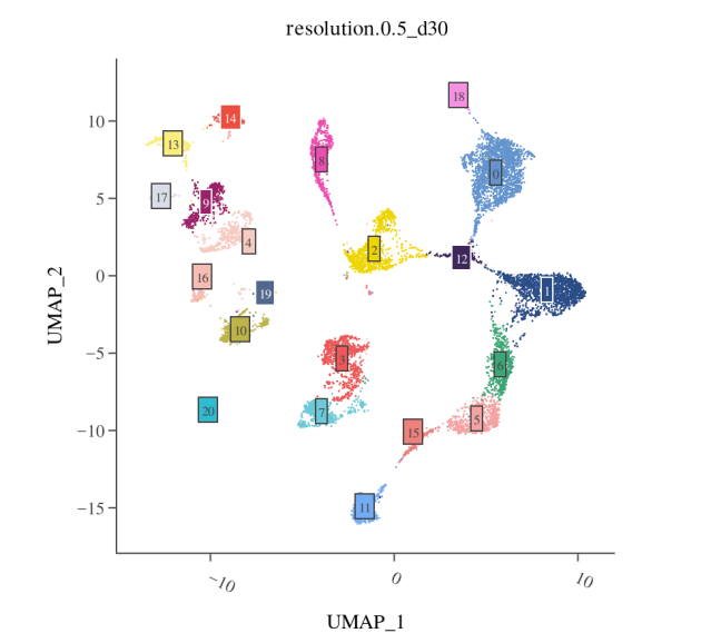

三. Dimensionality Reduction and Clustering on the ATAC Modality

1) TF-IDF Normalization and Feature Selection

• TF-IDF Transformation: scATAC-seq data consists of sparse count matrices. The RunTFIDF() function is used to normalize peak counts for each cell. This approach reduces the influence of peaks that are open in most cells (which lack specificity), and also helps mitigate batch effects caused by differences in sequencing depth.

• Top Features Selection: The FindTopFeatures() function is typically used to select peaks above the lowest quantile (e.g., min.cutoff = 'q0'). This reduces computational burden, improves the quality of dimensionality reduction, and significantly boosts the efficiency of subsequent LSI calculations.

2) LSI Dimensionality Reduction

• Latent Semantic Indexing (LSI): Similar to PCA, LSI reduces the high-dimensional peak matrix to a lower-dimensional space, usually into 50 LSI components.

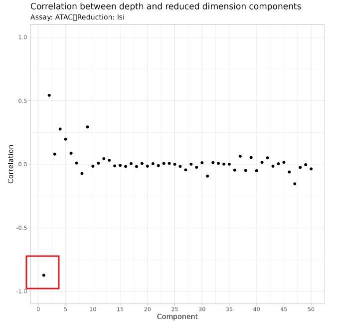
  TIP

  • LSI_1 mainly captures differences in sequencing depth rather than cell type differences. Including LSI_1 may cause clustering results to be dominated by sequencing depth rather than true biological variation.
  • Starting from LSI_2 provides a more accurate reflection of biologically meaningful chromatin state differences.

3) UMAP Visualization and Clustering

• UMAP Dimensionality Reduction: Projects high-dimensional data into a 2D space to facilitate intuitive observation of cell distribution and clustering results.

• Clustering Analysis: Constructs a K-nearest neighbor (KNN) graph in the lsi space and performs clustering using the FindNeighbors() and FindClusters() functions.

library(Signac)

# TF-IDF Transformation and Feature Selection on the ATAC Modality
data <- RunTFIDF(data, assay = "ATAC")
data <- FindTopFeatures(data, assay = "ATAC", min.cutoff = 'q0')
# LSI dimensionality reduction
data <- RunSVD(data, assay = "ATAC", reduction.key = "LSI_", n = 50)
# UMAP dimensionality reduction (alternatively, you can use `RunTSNE()` for t-SNE dimensionality reduction)
data <- RunUMAP(data, reduction = "lsi", dims = 2:50, reduction.name = "umap.atac")
# Clustering Analysis
data <- FindNeighbors(data, reduction = "lsi", dims = 2:50)
data <- FindClusters(data, resolution = 0.6)

# ATAC Visualization
DimPlot(data, reduction = "umap.atac", label = TRUE)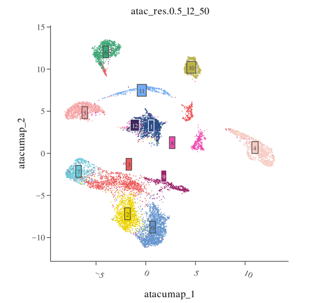

四. Joint Dimensionality Reduction: WNN (Weighted Nearest Neighbors)

1) Principle of WNN

• Core Idea of Weighted Nearest Neighbors: For each cell, WNN simultaneously considers its nearest neighbors in both the RNA and ATAC modalities, dynamically adjusting the weights based on the amount of informative signal from each modality.

• Weight Calculation Mechanism: If a cell contains more informative and distinctive features in the RNA modality (i.e., it is more distinguishable from other cells by RNA expression), the RNA weight will be higher; conversely, if the ATAC modality provides more reliable information, ATAC will receive a higher weight. Adaptive weighting allows WNN to fully leverage the advantages of both modalities while minimizing the interference from weaker modalities.

2) Steps to Implement WNN

• Step 1: Construct the Weighted Nearest Neighbor Graph

obj <- FindMultiModalNeighbors(
  obj,
  reduction.list = list("pca", "lsi"),
  dims.list = list(1:30, 2:50)
)

Parameter explanation:

• reduction.list: Specifies the list of dimensionality reduction results to use for building the neighbor graph (RNA and ATAC).

• dims.list: Specifies the range of dimensions used for RNA and ATAC, respectively. Note that for ATAC, it starts from the 2nd dimension.

• Step 2: Perform UMAP dimensionality reduction in the WNN space

obj <- RunUMAP(
  obj, 
  nn.name = "weighted.nn",
  reduction.name = "wnn.umap", 
  reduction.key = "wnnUMAP_"
)

Parameter explanation:

• nn.name: Specifies which neighbor graph to use; here, weighted.nn is selected.

• reduction.name: Name to save the dimensionality reduction result, used for downstream visualization.

• Step 3: Clustering Based on the WNN Graph

obj <- FindClusters(
  obj, 
  graph.name = "wnn", 
  resolution = 0.4, 
  algorithm = 3  # 3 stands for the Leiden algorithm
)

Parameter explanation:

• graph.name: Specifies to use the wnn graph (weighted shared nearest neighbor graph) for clustering.
• resolution: The clustering resolution; a higher value results in more clusters. It is recommended to start testing from 0.2.
• algorithm: The clustering algorithm; 3 corresponds to the Leiden algorithm (recommended).

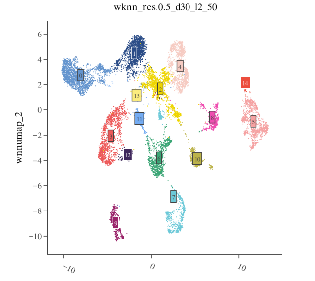
3) Visualization and Validation of WNN Results

五. Frequently Asked Questions

Q1: Why does ATAC LSI dimensionality reduction start from the 2nd dimension instead of the 1st?

A: The first dimension of LSI (LSI_1) mainly captures sequencing depth variation rather than biological variability. This differs from PCA, where the first principal component usually contains the most biological information. In ATAC-seq data, sequencing depth can vary greatly (from thousands to tens of thousands of fragments), and LSI_1 reflects this technical variation rather than true cell type differences. If LSI_1 is used, clustering results may be dominated by sequencing depth, leading to clusters of high-depth and low-depth cells, which does not reflect true cell types. Therefore, starting from LSI_2 allows for more accurate capture of biological variation.

Q2: Is it normal for clustering results of RNA and ATAC modalities to be inconsistent?

A: Yes, this is normal and commonly observed. RNA and ATAC capture different types of information:

• RNA reflects transcriptional output, influenced by transcriptional activity, RNA stability, and other factors.
• ATAC reflects chromatin accessibility, influenced by transcription factor binding, epigenetic modifications, etc.

Therefore, the clustering results of the two modalities may differ:

• If the difference is small, it suggests the information from both modalities is consistent, and cell types are clearly separated at both the transcriptional and regulatory levels.
• If the difference is large, this might indicate:
  1. Some cell subpopulations share similar transcriptional states but differ in regulatory states (or vice versa)—a situation where joint dimensionality reduction is especially beneficial.
  2. Data quality issues, making one modality unreliable.
  3. Biological reality, such as certain cells being in a transitional state with asynchronous transcription and regulation.

It is recommended to review RNA, ATAC, and WNN clustering results together; WNN typically provides the most robust results.

Q3: How can I validate if the WNN joint dimensionality reduction results are reasonable?

A: You can validate them from the following aspects:

1. Consistency with known marker genes: Check whether known cell type marker genes (e.g., CD3D for T cells, MS4A1 for B cells) are highly expressed in the corresponding WNN clusters.

2. Consistency between RNA and ATAC: Compare the clustering results of RNA, ATAC, and WNN, and see if WNN has appropriately integrated information from both modalities. If WNN clustering matches both RNA and ATAC clusters to some extent, the integration can be considered reasonable.

3. Biological plausibility: Check if the clustering results are consistent with biological expectations. For example, cell types related to the same developmental lineage should be adjacent in UMAP space; functionally similar cell types should cluster together.