ATAC + RNA Multi-omics: ATAC-Based Monocle3 Analysis

Author: SeekGene

Time: 42 min

Words: 8.4k words

Updated: 2026-07-07

Reads: 0 times

1. Tutorial Overview

This tutorial leverages single-cell ATAC-seq (scATAC-seq) data and the Monocle3 trajectory inference algorithm to reconstruct the continuous developmental or differentiation process of cells from "start" to "end." The core idea of pseudotime analysis is: to order discrete cells in high-dimensional space along an implicit biological progress trajectory, thereby revealing the dynamic patterns of gene regulation, chromatin accessibility, and transcription factor activity throughout this process.

This tutorial revolves around three core modalities, systematically reconstructing the complete logical chain of "regulatory initiation → chromatin changes → gene expression":

• Peak (Chromatin Accessibility Peak): Represents cis-regulatory elements in the genome (e.g., enhancers, promoters), whose accessibility dynamically changes along pseudotime.
• Motif (Transcription Factor Binding Motif): DNA sequence patterns enriched within accessible Peaks, reflecting the potential binding activity of TFs at the chromatin level.
• Gene (Gene Expression): The ultimate functional output of regulatory events at the transcriptional level, displaying spatiotemporally specific expression patterns along pseudotime.

Analysis Pipeline Overview:

1. Trajectory Inference: Based on dimensionality-reduction embedding (UMAP), Monocle3 learns the Principal Graph structure between cell states, and computes pseudotime values for each cell starting from a designated root cell population.
2. Differential Accessibility Peak Detection: Using generalized linear models (GLM), identify Peaks that change significantly along pseudotime.
3. Differential Motif Activity (chromVAR) Detection: Compute the chromatin accessibility deviation value of each TF Motif in every cell, and evaluate its significant change along pseudotime via a linear model.
4. Differentially Expressed Gene Detection (graph_test): Based on the Monocle3 Principal Graph topology, detect genes displaying spatial autocorrelation along pseudotime.
5. Multi-Modal Joint Visualization: Integrate the dynamic changes of RNA, Motif, and Peak along pseudotime into the same heatmap framework, enabling global display of cross-modal signal transmission.

💡 Note: The figures shown in the documentation represent only a subset of representative visualizations. For the complete analysis results across all cell populations or comparison groups (including detailed data tables and all high-resolution plots), please refer to the ./output/ directory.

suppressPackageStartupMessages({
    library(Signac)
    library(Seurat)
    library(SeuratWrappers)
    library(SummarizedExperiment)
    library(monocle3)
    library(cicero)
    library(Matrix)
    library(ggplot2)
    library(patchwork)
    library(parallel)
    library(Biostrings)
    library(TFBSTools)
    library(JASPAR2020)
    library(GenomeInfoDb)
    library(ComplexHeatmap)
    library(circlize)
})

2. Input File Preparation

2.1 Input File Preparation and Parameter Configuration

Before running the analysis, please ensure that the following input files and parameters are properly configured. A unified parameter configuration section is provided at the top of the script; users can modify it according to their actual project needs:

• input.rds: Pre-processed single-cell ATAC-seq Seurat object (must contain ATAC Assay, clustering information, and UMAP dimensionality reduction results).
• meta.tsv (optional): Additional cell metadata file containing a barcodes column and extra annotation columns.
• genome.fa: Reference genome FASTA file for the corresponding species, used for background correction in chromVAR Motif activity analysis.

💡 Note Parameters here need to be filled in according to the actual situation of your own data, especially file paths, species information, and target cell types. All paths are recommended to be absolute paths to avoid working directory confusion.

## outdir: Output directory path; all analysis results (plots, tables) will be saved in the output subfolder under this directory
outdir = "./"

## ref_genome: Path to the reference genome FASTA file, used for GC-content background correction in chromVAR Motif activity analysis
ref_genome = "/path/to/genome.fa"

## rds: Path to the input Seurat object RDS file; must contain both ATAC and RNA assays along with preprocessing results
rds = "/path/to/input.rds"

## meta: (Optional) Path to the cell metadata TSV file; must contain a barcodes column for matching with the Seurat object
meta = "/path/to/meta.tsv"

## Reduction: Dimensionality-reduction embedding method used for trajectory inference; options include "UMAP", "ATACUMAP", "WNNUMAP" (case-insensitive)
Reduction = "WNNUMAP"

## species: Species information, "human" or "mouse" etc., used to automatically select the corresponding JASPAR Motif database
species = "human"

## root: Name of the cell type designated as the pseudotime starting point; must exist in the column corresponding to clusters_col
root = "CMP"

## clusters_col: Name of the column in the Seurat object's meta.data that stores cell type / cluster information
clusters_col = "Celltype"

## celltypes: Comma-separated list of cell types to be analyzed; only cells of these types are retained for analysis
celltypes = "Monocytes,Pro B cells,CMP"

## sample_col: Name of the column in the Seurat object's meta.data that stores sample origin information
sample_col = "Sample"

## samples: Comma-separated list of sample IDs to be analyzed; used to filter cells from specific samples
samples = "25030508_pbmc_1_arc,25030508_pbmc_1_arc"

## use_partition: Whether to use Monocle3's partition information for trajectory learning; TRUE or FALSE
use_partition = "TRUE"

## downsample: Whether to downsample cells to reduce computational load; TRUE or FALSE
downsample = "FALSE"

## downsample_num: When downsampling is enabled, the maximum number of cells retained per cell type
downsample_num = "1000"

💡 Note: For the first analysis, it is not recommended to modify the use_partition and downsample parameters. use_partition = TRUE will automatically partition by connected components for trajectory inference when the number of cells is large, helping to improve learning efficiency on large-scale data; downsample = FALSE retains all cells to maximize trajectory resolution.

⚠️ Note:

• The cell type specified by the root parameter must exist in the celltypes list; otherwise, trajectory ordering will fail.
• The name of the Reduction parameter (e.g., "WNNUMAP") must exactly match the key name in obj@reductions of the Seurat object (this tool supports case-insensitive matching).

2.2 Auxiliary Parameters

Configure auxiliary parameters used in plotting and analysis.

Core Parameter Descriptions:

• n_bins: Number of bins to divide the pseudotime range into (default 10), used for cell binning in Peak differential analysis.
• top_n_heatmap: Maximum total number of differential features (RNA/Motif/Peak) displayed in the heatmap.

n_bins <- 10
top_n_heatmap <- 100
my36colors <- c(
  "#E5D2DD", "#53A85F", "#F1BB72", "#F3B1A0", "#D6E7A3", "#57C3F3", "#476D87",
  "#E95C59", "#E59CC4", "#AB3282", "#23452F", "#BD956A", "#8C549C", "#585658",
  "#9FA3A8", "#E0D4CA", "#5F3D69", "#C5DEBA", "#58A4C3", "#E4C755", "#F7F398",
  "#AA9A59", "#E63863", "#E39A35", "#C1E6F3", "#6778AE", "#91D0BE", "#B53E2B",
  "#712820", "#DCC1DD", "#CCE0F5", "#CCC9E6", "#625D9E", "#68A180", "#3A6963",
  "#968175", "#6495ED", "#FFC1C1", "#f1ac9d", "#f06966", "#dee2d1", "#6abe83",
  "#39BAE8", "#B9EDF8", "#221a12", "#b8d00a", "#74828F", "#96C0CE", "#E95D22",
  "#017890"
)

2.3 Output Directory Initialization and Parameter Parsing

Before entering the formal analysis, create the output directory and convert string parameters to R native types.

Core Steps Breakdown:

1. Directory Creation: Create the output/ subdirectory under the main output directory; all analysis artifacts are saved here.
2. String Splitting: Split the comma-separated celltypes and samples strings into character vectors.
3. Type Conversion: Convert "TRUE"/"FALSE" strings to logical values, and downsample_num to numeric.

⚠️ Note: Parameter validation is executed immediately after conversion; if type conversion of downsample_num, use_partition, or downsample fails (returning NA), a clear error message will be raised.

# ---- Cell 4 ----
outdir <- paste0(outdir, "/output")
dir.create(outdir, recursive = TRUE, showWarnings = FALSE)

celltypes <- strsplit(celltypes, ",")[[1]]
celltypes <- trimws(celltypes)
samples <- strsplit(samples, ",")[[1]]

use_partition <- as.logical(use_partition)
downsample <- as.logical(downsample)
downsample_num <- as.numeric(downsample_num)
if (is.na(downsample_num)) stop("downsample_num must be numeric.")
if (is.na(use_partition)) stop("use_partition must be TRUE/FALSE.")
if (is.na(downsample)) stop("downsample must be TRUE/FALSE.")

2.4 Helper Functions

Before entering the formal analysis, first define a set of helper functions that will be repeatedly used throughout the pipeline. These functions handle name normalization, dimensionality-reduction mapping resolution, feature selection, matrix smoothing, and plotting of various visualization types.

💡 Note: The following functions are internal implementations of this tutorial and do not involve modifications to core statistical methods. Each function has a clear input/output contract and can be independently reused.

(1) Name Normalization Function Used for fuzzy matching of dimensionality-reduction embedding names (case-insensitive).

normalize_name <- function(x) {
  gsub("[^a-z0-9]", "", tolower(x))
}

(2) Dimensionality-Reduction Embedding Resolution Function

1. Extract all available dimensionality-reduction result names from the Seurat object.
2. Normalize the user-input reduction_name (remove special characters, unify to lowercase).
3. Match against the available list to find the corresponding original key name.

⚠️ Note: If the specified dimensionality reduction method does not exist, the function will list all available reduction names for debugging. Common available options include umap, ATACUMAP, WNNUMAP, etc.

resolve_reduction <- function(obj, reduction_name) {
  available <- names(obj@reductions)
  if (length(available) == 0) {
    stop("No reductions found in Seurat object.")
  }
  normalized_available <- normalize_name(available)
  target <- normalize_name(reduction_name)
  idx <- match(target, normalized_available)
  if (is.na(idx)) {
    stop(
      paste0(
        "Reduction '", reduction_name, "' not found. Available reductions: ",
        paste(available, collapse = ", ")
      )
    )
  }
  available[idx]
}

(3) Feature Column Auto-Selection Function In different analysis steps, the column name of differential result tables may be site_name, id, or feature_id. This function automatically identifies and returns the first matching column name.

pick_feature_col <- function(df, candidates) {
  existing <- intersect(candidates, colnames(df))
  if (length(existing) == 0) {
    stop(paste0("Feature column not found. Candidates: ", paste(candidates, collapse = ", ")))
  }
  existing[1]
}

(4) Multi-Modal CDS Switching Function

The CellDataSet (CDS) object of Monocle3 binds by default to one modality's count matrix (in this tutorial, ATAC accessibility). However, during differential gene analysis, we need to apply the same trajectory topology to the RNA expression matrix to detect dynamic changes in gene expression along pseudotime.

This function replaces the CDS's count matrix from ATAC to RNA while keeping the Principal Graph structure and dimensionality-reduction embeddings unchanged, achieving one trajectory framework, multi-modal analysis.

Core Steps Breakdown:

1. Extract the normalized expression matrix of the specified Assay (e.g., "RNA") from the Seurat object.
2. Create a new CDS object, replacing only the expression_data field.
3. Fully inherit the original CDS's reducedDims, principal_graph, and principal_graph_aux.

💡 Note: This "modality switching" is a standard paradigm for Monocle3 multi-omics analysis: the trajectory is learned using ATAC, and gene expression is tested along the same trajectory via graph_test.

swap_cds_assay <- function(main_cds, seurat_obj, assay) {
  common_cells <- intersect(colnames(main_cds), colnames(seurat_obj))
  main_cds <- main_cds[, common_cells]
  mat <- GetAssayData(seurat_obj, assay = assay, layer = "data")
  mat <- mat[, common_cells]
  
  new_cds <- new_cell_data_set(
    expression_data = mat,
    cell_metadata = colData(main_cds),
    gene_metadata = data.frame(gene_short_name = rownames(mat), row.names = rownames(mat))
  )
  reducedDims(new_cds) <- reducedDims(main_cds)
  new_cds@principal_graph_aux <- main_cds@principal_graph_aux
  new_cds@principal_graph <- main_cds@principal_graph
  return(new_cds)
}

(5) Pseudotime-Smoothed Matrix Construction Function

Core Steps Breakdown:

1. Pseudotime Ordering: Sort all valid cells from smallest to largest by pseudotime value.
2. Equidistant Sampling: Uniformly generate n_points (default 100) sampling points across the pseudotime range [min(pt), max(pt)].
3. Neighborhood-Mean Smoothing: For each sampling point, select the K nearest cells (at least 10, or 5% of the total cell count) and compute the mean of their feature expression. This step effectively eliminates the sparse noise (Drop-out) of single-cell data.
4. Z-score Normalization: Row-wise (feature-wise) Z-score normalize the smoothed matrix, making the relative change trends of different features comparable on the same scale.

💡 Note: The smoothed matrix is a key intermediate product for heatmap visualization. It transforms discrete cell expression data into continuous signal curves along pseudotime, enabling precise alignment and comparison of heatmaps across the RNA, Motif, and Peak modalities.

build_smoothed_matrix <- function(mat, pt, features, n_points = 100) {
  features <- intersect(features, rownames(mat))
  if (length(features) == 0) return(NULL)
  
  common_cells <- intersect(colnames(mat), names(pt))
  pt <- pt[common_cells]
  valid <- is.finite(pt)
  common_cells <- common_cells[valid]
  pt <- pt[valid]
  
  ord <- order(pt)
  common_cells <- common_cells[ord]
  pt <- pt[ord]
  m <- mat[features, common_cells, drop = FALSE]
  pt_seq <- seq(min(pt), max(pt), length.out = n_points)
  
  smooth_m <- matrix(0, nrow = length(features), ncol = n_points)
  rownames(smooth_m) <- features
  colnames(smooth_m) <- paste0("P", 1:n_points)
  
  for (i in 1:n_points) {
    dist <- abs(pt - pt_seq[i])
    idx <- order(dist)[1:max(10, floor(length(pt)*0.05))]
    smooth_m[, i] <- Matrix::rowMeans(m[, idx, drop=FALSE])
  }
  
  z <- t(scale(t(smooth_m)))
  z[is.na(z)] <- 0
  return(list(z = z, pseudotime = pt_seq))
}

(6) Complex Heatmap Plotting Function

This function plots a feature dynamic change heatmap along pseudotime based on ComplexHeatmap.

Core Steps Breakdown:

1. Motif Name Mapping: Map internal Motif IDs (e.g., MA0001.1) to human-readable TF names (e.g., SP1).
2. Pseudotime Color Bar: Add a pseudotime gradient color bar (deep purple → cyan-green → bright yellow) at the top of the heatmap, intuitively annotating cell positions on the trajectory.
3. Key Feature Annotation: Use anno_mark to automatically annotate the names of Top features with the largest effect values, linking them to the corresponding heatmap rows via connecting lines.

💡 Note: Heatmap rows are partitioned into row_km = 2 groups by K-means, typically representing the "up-regulated along pseudotime" and "down-regulated along pseudotime" feature clusters respectively.

plot_complex_heatmap <- function(z_obj, title_text, top_labels, motif_names = NULL) {
  if (is.null(z_obj)) return(NULL)
  z_mat <- z_obj$z
  pt_vec <- z_obj$pseudotime
  
  if (!is.null(motif_names)) {
    rn <- rownames(z_mat)
    mapped <- motif_names[rn]
    rn <- ifelse(is.na(mapped), rn, mapped)
    rownames(z_mat) <- rn
    
    mapped_top <- motif_names[top_labels]
    top_labels <- ifelse(is.na(mapped_top), top_labels, mapped_top)
  }
  
  col_fun <- colorRamp2(c(-2, 0, 2), c("#2166AC", "#F7F7F7", "#B2182B"))
  pt_range <- range(pt_vec, na.rm = TRUE)
  if (!all(is.finite(pt_range)) || diff(pt_range) == 0) {
    pt_range <- c(0, 1)
  }
  pt_col_fun <- colorRamp2(
    c(pt_range[1], mean(pt_range), pt_range[2]),
    c("#440154", "#21908C", "#FDE725")
  )
  top_anno <- HeatmapAnnotation(
    Pseudotime = pt_vec,
    col = list(Pseudotime = pt_col_fun),
    show_annotation_name = TRUE
  )
  
  idx <- which(rownames(z_mat) %in% top_labels)
  row_anno <- NULL
  if (length(idx) > 0) {
    row_anno <- rowAnnotation(
      link = anno_mark(at = idx, labels = rownames(z_mat)[idx], labels_gp = gpar(fontsize = 8))
    )
  }
  
  ht <- Heatmap(
    z_mat,
    name = "Z-score",
    column_title = title_text,
    cluster_columns = FALSE,
    cluster_rows = TRUE,
    row_km = 2,
    col = col_fun,
    show_row_names = FALSE,
    show_column_names = FALSE,
    top_annotation = top_anno,
    right_annotation = row_anno,
    use_raster = TRUE,
    raster_quality = 3
  )
  return(ht)
}

(7) Top Feature Scatter Plot Function

Plot single-cell expression scatter plots of Top features (RNA genes, Motifs, or Peaks) along pseudotime, with a LOESS smoothed curve overlaid.

Core Steps Breakdown:

1. Data Alignment: Align the feature matrix, pseudotime vector, and cell-type annotation to a common cell set.
2. Faceted Visualization: Use facet_wrap to generate an independent subplot for each feature, facilitating individual evaluation of its dynamic pattern.
3. LOESS Trend Line: Overlay a LOESS smoothed curve (black) on each subplot, intuitively displaying the overall change direction of the feature along pseudotime.

💡 Note:

• Scatter Point Colors: Mapped from cell-type annotation, helping identify which cell subpopulations contribute the main signal for that feature.
• LOESS Curve: Reflects the overall trend direction of the feature. Curve upward = up-regulated along pseudotime; curve downward = down-regulated along pseudotime.

plot_top_feature_scatter <- function(
  mat,
  features,
  pseudotime_vec,
  cell_types,
  ct_colors,
  title_prefix,
  y_label,
  out_prefix,
  outdir
) {
  features <- unique(features)
  features <- features[features %in% rownames(mat)]
  if (length(features) == 0) return(invisible(NULL))

  common_cells <- intersect(colnames(mat), names(pseudotime_vec))
  common_cells <- intersect(common_cells, names(cell_types))
  pt <- pseudotime_vec[common_cells]
  valid <- is.finite(pt)
  common_cells <- common_cells[valid]
  pt <- as.numeric(pt[valid])
  ct <- as.character(cell_types[common_cells])

  plot_df_list <- lapply(features, function(feat) {
    y <- as.numeric(mat[feat, common_cells])
    data.frame(
      feature = feat,
      pseudotime = pt,
      value = y,
      celltype = ct,
      stringsAsFactors = FALSE
    )
  })
  plot_df <- do.call(rbind, plot_df_list)
  if (nrow(plot_df) == 0) return(invisible(NULL))

  plot_df$feature <- factor(plot_df$feature, levels = features)
  plot_df$celltype <- factor(plot_df$celltype, levels = names(ct_colors))

  p <- ggplot(plot_df, aes(x = pseudotime, y = value, color = celltype)) +
    geom_point(size = 0.6, alpha = 0.75) +
    geom_smooth(aes(group = feature), method = "loess", se = FALSE, color = "black", linewidth = 0.6) +
    facet_wrap(~feature, scales = "free_y", ncol = 2) +
    scale_color_manual(values = ct_colors, drop = FALSE) +
    labs(x = "pseudotime", y = y_label, title = title_prefix, color = "CellType") +
    theme_bw(base_size = 11) +
    theme(
      panel.grid = element_blank(),
      strip.background = element_rect(fill = "white"),
      plot.title = element_text(hjust = 0.5)
    )
  print(p) 
  ggsave(file.path(outdir, paste0(out_prefix, ".png")), plot = p, width = 10, height = 12, dpi = 300)
  ggsave(file.path(outdir, paste0(out_prefix, ".pdf")), plot = p, width = 10, height = 12)
}

3. Data Loading and Preprocessing

3.1 Reading the Seurat Object

Load the pre-processed single-cell ATAC-seq data from the RDS file. If an additional metadata file (meta.tsv) is provided, merge it into the Seurat object by barcode.

obj <- readRDS(rds)
if (meta != "") {
  meta_df <- read.table(meta, header = TRUE, sep = "\t", check.names = FALSE)
  rownames(meta_df) <- meta_df$barcodes
  obj <- AddMetaData(obj, meta_df)
}

3.2 Cell Type and Sample Selection

• Retain only cell types in the clusters_col column that match the celltypes list.
• Retain only samples in the sample_col column that match the samples list.

obj@meta.data[[clusters_col]] <- as.character(obj@meta.data[[clusters_col]])
obj <- subset(obj, subset = !!sym(clusters_col) %in% celltypes)
obj <- subset(obj, subset = !!sym(sample_col) %in% samples)

3.3 Downsample Balancing

If downsample = TRUE, perform random downsampling by downsample_num on each cluster to reduce computational burden.

DefaultAssay(obj) <- "ATAC"
Idents(obj) <- obj@meta.data[[clusters_col]]
if (downsample) {
  obj <- subset(obj, cells = WhichCells(obj, downsample = downsample_num))
}

⚠️ Note:

• If the number of cells after filtering is too small (e.g., < 50), Monocle3's graph learning algorithm may fail to converge. It is recommended to check the total cell count after filtering before running.
• The meta.tsv file must contain a barcodes column, and its values must be consistent with the cell barcodes in the Seurat object.

4. Monocle3 Trajectory Inference

4.1 Dimensionality-Reduction Embedding Mapping

Monocle3 internally uses UMAP as the dimensionality-reduction coordinates. Since dimensionality-reduction results in the Seurat object may be named WNNUMAP or ATACUMAP, we need to extract them and re-register them as the "UMAP" reduction recognizable by Monocle3.

Core Steps Breakdown:

1. Reduction Name Resolution: Call the resolve_reduction() function to match the user-specified Reduction name to the actual key name in the Seurat object (case-insensitive).
2. Extract Embedding Coordinates: Obtain the coordinate matrix of all cells under that dimensionality reduction.
3. Create Monocle3-Compatible Reduction: Register the extracted coordinates as the "umap" reduction.

# ---- Cell 6 ----
selected_reduction <- resolve_reduction(obj, Reduction)
umap_embed <- Embeddings(obj, reduction = selected_reduction)
obj[["umap"]] <- CreateDimReducObject(
  embeddings = umap_embed,
  key = "UMAP_",
  assay = DefaultAssay(obj)
)

💡 Note: Monocle3 has strict requirements on the reduction key name (must contain "UMAP"). Directly using non-standard names will cause learn_graph() to raise an error.

4.2 CDS Conversion and Principal Graph Learning

Core Steps Breakdown:

1. Seurat → CDS Conversion: Use as.cell_data_set() to convert the Seurat object to Monocle3's CellDataSet object. This is the data structure foundation for all Monocle3 analyses.
2. UMAP Coordinate Injection: Write the previously extracted UMAP embedding coordinates directly into the CDS's reducedDims, ensuring that Monocle3 uses dimensionality-reduction results consistent with ours.
3. Gene Detection: Call detect_genes() to mark genes/features expressed in each cell, providing the background set for subsequent differential analysis.
4. Cell Clustering: Perform cluster_cells() based on UMAP coordinates to identify cell state populations.
5. Principal Graph Learning (learn_graph): Monocle3's core algorithm — learn the graph structure (Principal Graph) connecting each cell state population in the dimensionality-reduced space. The use_partition parameter controls whether to use partition mode in large datasets.
6. Pseudotime Ordering (order_cells): Using the designated root cell population as the starting point, compute the pseudotime value of each cell along the Principal Graph.
7. Result Saving: Save the complete CDS object as an RDS file, and inject the pseudotime values back into the Seurat object's metadata.

💡 Note:

• Root Cell Selection: The cell type specified by the root parameter must be a biologically plausible developmental starting point (e.g., stem cells, progenitor cells). Choosing an incorrect root cell will cause the entire pseudotime direction to be reversed.
• Partition Mode: When cells have multiple disconnected developmental branches, use_partition = TRUE will automatically split the data into independent partitions for separate learning. If use_partition = FALSE is forced, Monocle3 will attempt to connect all cells into a single graph, potentially causing unreasonable cross-lineage connections.

counts_mat <- GetAssayData(obj, assay = "ATAC", layer = "counts")

counts_mat <- as(counts_mat, "dgCMatrix")

cds <- new_cell_data_set(
  expression_data = counts_mat,
  cell_metadata = obj@meta.data,
  gene_metadata = data.frame(
    gene_short_name = rownames(counts_mat),
    row.names = rownames(counts_mat)
  )
)

reducedDims(cds)$UMAP <- umap_embed[colnames(cds), , drop = FALSE]

cds <- detect_genes(cds)
cds <- cluster_cells(cds = cds, reduction_method = "UMAP")
cds <- learn_graph(cds, use_partition = use_partition)

root_cells <- rownames(obj@meta.data[obj@meta.data[[clusters_col]] == root, ])
if (length(root_cells) == 0) {
  stop("No root cells found. Check root and clusters_col.")
}
cds <- order_cells(cds, reduction_method = "UMAP", root_cells = root_cells)
saveRDS(cds, file.path(outdir, "cds.rds"))

pseudotime_vec <- pseudotime(cds)
obj <- AddMetaData(obj, metadata = pseudotime_vec, col.name = "Monocle3_pseudotime")

output

|======================================================================| 100%

4.3 Trajectory Visualization

Map pseudotime and cell type onto UMAP respectively, generating a four-panel plot (with/without trajectory graph × two coloring schemes).

Output Files:

• pseudotime.png/pdf: Left panel shows pseudotime gradient + trajectory skeleton; right panel shows pseudotime gradient only.
• celltype.png/pdf: Left panel shows cell-type distribution + trajectory skeleton; right panel shows cell-type distribution only.

💡 Note: Comparing the pseudotime plot and cell-type plot can help you verify: whether the trajectory direction is consistent with the expected developmental order of each cell type (e.g., progenitor → intermediate → terminally differentiated cell).

p1 <- plot_cells(
  cds = cds,
  color_cells_by = "pseudotime",
  label_cell_groups = FALSE,
  show_trajectory_graph = TRUE
)

p2 <- plot_cells(
  cds = cds,
  color_cells_by = "pseudotime",
  label_cell_groups = FALSE,
  show_trajectory_graph = FALSE
)
p3 <- plot_cells(
  cds = cds,
  color_cells_by = clusters_col,
  show_trajectory_graph = TRUE,
  label_cell_groups = FALSE
)
p4 <- plot_cells(
  cds = cds,
  color_cells_by = clusters_col,
  show_trajectory_graph = FALSE,
  label_cell_groups = FALSE
)
ggsave(p1 + p2, file = file.path(outdir, "pseudotime.png"), width = 12, height = 5, dpi = 300)
ggsave(p3 + p4, file = file.path(outdir, "celltype.png"), width = 12, height = 5, dpi = 300)
ggsave(p1 + p2, file = file.path(outdir, "pseudotime.pdf"), width = 12, height = 5)
ggsave(p3 + p4, file = file.path(outdir, "celltype.pdf"), width = 12, height = 5)

options(repr.plot.width = 14, repr.plot.height = 7)
p1 + p2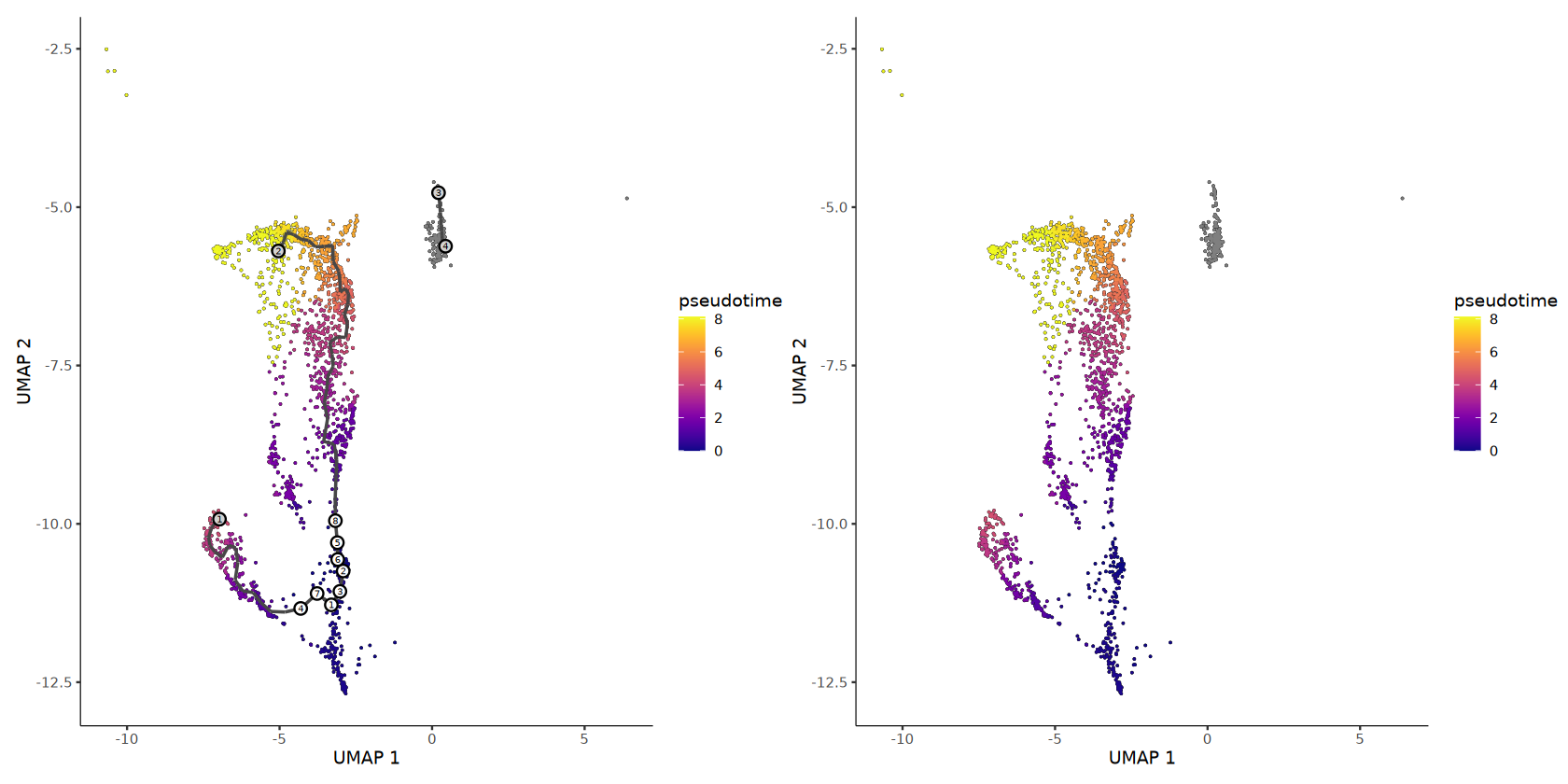

options(repr.plot.width = 14, repr.plot.height = 7)
p3 + p4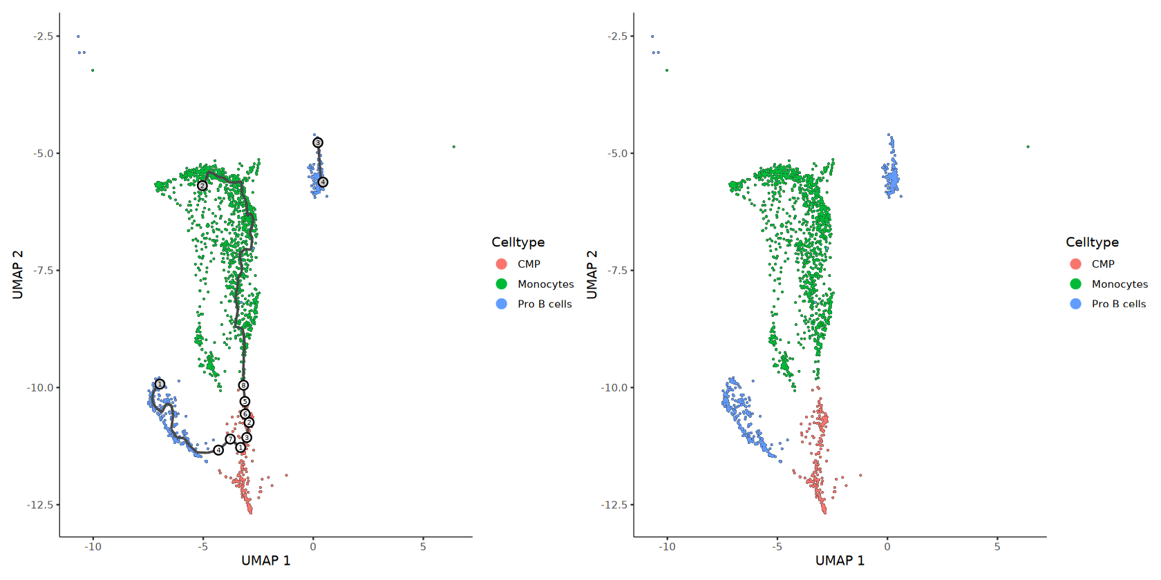

5. Multi-Omics Dynamic Feature Detection (Along Pseudotime)

Use Monocle3's fit_models() function to evaluate with a generalized linear model (GLM) whether the accessibility of each Peak changes significantly along pseudotime.

5.1 Differential Chromatin Accessibility Analysis Along Pseudotime

Core Steps Breakdown:

1. Filter Invalid Cells: Retain only cells with finite pseudotime values (excluding cells that cannot be ordered).
2. Pseudotime Binning: Divide the pseudotime range into n_bins equal intervals, treating each interval as a "pseudo-sample."
3. Cell Aggregation: Call aggregate_by_cell_bin() to aggregate cells within the same bin into a pseudo-bulk sample, reducing sparsity.
4. GLM Fitting: Fit a generalized linear model for each Peak using the formula ~Pseudotime + num_genes_expressed. Wherein:
   • Pseudotime: The main effect term, evaluating the change of Peak accessibility along pseudotime.
   • num_genes_expressed: Covariate, correcting for sequencing depth differences.
5. Significance Filtering: Extract Peaks with term == "Pseudotime" and q_value < 0.05, saving as a CSV file.

💡 Note:

• q_value: P-value after Benjamini-Hochberg (BH) multiple-testing correction. q_value < 0.05 means significant at the 5% false discovery rate (FDR) level.
• Estimate Sign: A positive value indicates Peak accessibility increases along pseudotime (enhanced opening); a negative value indicates it decreases along pseudotime (progressively closing).

⚠️ Note: The computational cost of fit_models() is proportional to the number of Peaks. For datasets with > 50K Peaks, it is recommended to use the cores parameter to specify multi-threading for acceleration. This tutorial automatically uses 80% of the system's cores (capped at 25).

cores <- ifelse(detectCores() > 32, 25, trunc(0.8 * detectCores()))

input_cds_lin <- cds[, is.finite(pseudotime_vec[colnames(cds)])]
pData(input_cds_lin)$Pseudotime <- pseudotime(input_cds_lin)
pData(input_cds_lin)$cell_subtype <- cut(pseudotime(input_cds_lin), n_bins)
binned_input_lin <- aggregate_by_cell_bin(input_cds_lin, "cell_subtype")
acc_fits <- fit_models(
  binned_input_lin,
  cores = cores,
  model_formula_str = "~Pseudotime + num_genes_expressed"
)
fit_coefs <- coefficient_table(acc_fits)
significant_sites <- subset(fit_coefs, term == "Pseudotime" & q_value < 0.05)

important_cols <- intersect(
  c("site_name", "estimate", "normalized_effect", "p_value", "q_value"),
  colnames(significant_sites)
)
important_data <- significant_sites[, important_cols, drop = FALSE]
write.csv(
  important_data,
  file.path(outdir, "pseudotime_differentially_accessible_sites.csv"),
  row.names = FALSE
)
peak <- unique(important_data$site_name)

writeLines(
  as.character(peak),
  con = file.path(outdir, "peak.txt")
)

head(important_data)

A tibble: 6 × 5

site_name	estimate	normalized_effect	p_value	q_value
<chr>	<dbl>	<dbl>	<dbl>	<dbl>
chr14-69042674-69044104	0.1474021	0.21239396	1.579794e-07	0.021606051
chr16-30496998-30497771	1.3722741	0.00000000	2.556358e-07	0.034961780
chr16-71972739-71973671	1.6343574	0.00000000	5.002789e-08	0.006842215
chr17-76604881-76606067	1.3722741	0.00000000	2.556358e-07	0.034961780
chr2-85963580-85964391	3.7951820	0.03617204	2.921967e-08	0.003996345
chr4-106266040-106266712	1.3586657	0.00000000	9.671732e-08	0.013227641

5.2 Top Changing Peak Visualization

Sort significantly changing Peaks by effect size (estimate), separately extracting the Top 5 most significantly up-regulated and down-regulated Peaks, and plot their accessibility change curves along pseudotime.

Output Files:

• top_increasing.png/pdf: Top Peaks progressively opening along pseudotime.
• top_decreasing.png/pdf: Top Peaks progressively closing along pseudotime.

💡 Note: The genomic regions corresponding to these Peaks may contain key cis-regulatory elements (e.g., development-specific enhancers). Combined with downstream Motif analysis, the transcription factors driving these changes can be further revealed.

# ---- Cell 9: top changing peaks ----
# Plotting top increasing/decreasing point plots
peak_feature_col <- pick_feature_col(significant_sites, c("site_name", "id", "feature_id"))
positive_sites <- significant_sites[significant_sites$estimate > 0, , drop = FALSE]
negative_sites <- significant_sites[significant_sites$estimate < 0, , drop = FALSE]
top_increasing <- head(positive_sites[order(-positive_sites$estimate), , drop = FALSE], 5)
top_decreasing <- head(negative_sites[order(-abs(negative_sites$estimate)), , drop = FALSE], 5)
top_increasing <- top_increasing[!is.na(top_increasing[[peak_feature_col]]), ]
top_decreasing <- top_decreasing[!is.na(top_decreasing[[peak_feature_col]]), ]

if (nrow(top_increasing) > 0) {
  p5 <- plot_accessibility_in_pseudotime(input_cds_lin[top_increasing[[peak_feature_col]]])
  ggsave(p5, file = file.path(outdir, "top_increasing.png"), width = 5, height = 8, dpi = 300)
  ggsave(p5, file = file.path(outdir, "top_increasing.pdf"), width = 5, height = 8)
} else {
  message("No positive pseudotime peaks found after filtering; skip top_increasing plot.")
}

if (nrow(top_decreasing) > 0) {
  p6 <- plot_accessibility_in_pseudotime(input_cds_lin[top_decreasing[[peak_feature_col]]])
  ggsave(p6, file = file.path(outdir, "top_decreasing.png"), width = 5, height = 8, dpi = 300)
  ggsave(p6, file = file.path(outdir, "top_decreasing.pdf"), width = 5, height = 8)
} else {
  message("No negative pseudotime peaks found after filtering; skip top_decreasing plot.")
}

output

No negative pseudotime peaks found after filtering; skip top_decreasing plot.

p5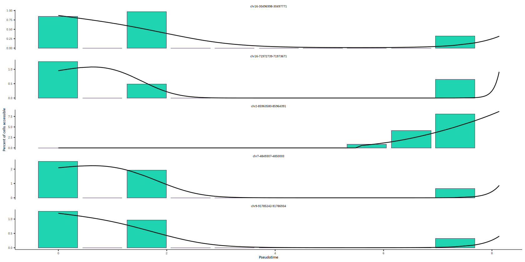

💡 Interpretation Guide

Global Description: top_increasing.png displays the 5 accessibility sites with the most significant increase along pseudotime, for observing the dynamic pattern of "progressive chromatin opening."

• X-axis (pseudotime): Represents the relative progress of cells along the trajectory from start to end; further right typically indicates closer to the terminal state.
• Y-axis (accessibility): Represents the accessibility intensity (raw or normalized value) of the corresponding peak; the higher the value, the more open the site.
• Trend Assessment: If the curve overall rises with pseudotime, it indicates the site is progressively activated during developmental progression and may participate in late-stage establishment.
• Cross-Site Comparison: Sites with steeper rise and higher terminal levels often suggest stronger stage-specific opening signals and can be prioritized for downstream validation.

#p6

💡 Interpretation Guide

Global Description: top_decreasing.png displays the 5 accessibility sites with the most significant decrease along pseudotime, reflecting the dynamic process of "progressive chromatin closing."

• X-axis (pseudotime): Represents the trajectory progress of cells from start to end; further right typically indicates closer to the terminal state.
• Y-axis (accessibility): Represents the accessibility level of the corresponding peak; decreasing values indicate that region is progressively closing.
• Trend Assessment: If the curve overall declines, it suggests the site is continuously inactivated during differentiation progression and may correspond to exit from early programs.
• Cross-Site Comparison: Sites with steeper decline and lower terminal levels typically have stronger stage-specific closing characteristics and can be key candidates.

5.3 Differential Gene Expression Analysis Along Pseudotime (RNA)

Changes in gene expression level are a direct reflection of cell state transitions. To identify genes that fluctuate significantly along pseudotime, the program switches to the RNA expression matrix for analysis:

• CDS Switching: Through the swap_cds_assay function, replace the CDS object's expression data with RNA Assay data, while retaining the original trajectory structure and dimensionality-reduction information, ensuring analysis proceeds within the same pseudotime framework.
• Low-Expression Gene Filtering: Remove genes expressed in fewer than 10 cells, reducing interference from sparse noise on the analysis.
• Spatial Autocorrelation Test: Use the graph_test function, with the Principal Graph (principal_graph) as the neighbor graph structure, to compute each gene's Moran's I statistic. Moran's I measures the spatial autocorrelation of gene expression in trajectory space — a high Moran's I value means gene expression shows a continuous, smooth change pattern along the trajectory, rather than a random distribution.
• Significant Gene Selection: Use dual thresholds of q_value < 0.05 and morans_I > 0.05 to select trajectory-related genes that are both statistically significant and biologically meaningful.

Analysis results are saved as pseudotime_differentially_expressed_genes.csv, and the gene list is also output as genes.txt for subsequent functional enrichment analysis or cross-validation with other omics data.

# ---- Cell 11: differential genes along pseudotime ----
cds_rna <- swap_cds_assay(cds, obj, "RNA")
# Filter genes expressed in at least 10 cells to speed up graph_test
cds_rna <- cds_rna[Matrix::rowSums(SingleCellExperiment::counts(cds_rna) > 0) > 10, ]
rna_graph_res <- graph_test(cds_rna, neighbor_graph="principal_graph", cores=cores)
significant_genes <- subset(rna_graph_res, q_value < 0.05 & morans_I > 0.05)

write.csv(
  as.data.frame(significant_genes),
  file.path(outdir, "pseudotime_differentially_expressed_genes.csv"),
  row.names = FALSE
)

gene_list <- unique(as.character(significant_genes$gene_short_name))
gene_list <- gene_list[!is.na(gene_list) & nzchar(gene_list)]

writeLines(gene_list, con = file.path(outdir, "genes.txt"))

5.4 Differential Motif Activity Analysis Along Pseudotime

Transcription factors regulate gene expression by binding to specific DNA motifs; the dynamic changes in their binding activity are key to understanding upstream regulatory logic. This tutorial uses the Motif activity matrix inferred by chromVAR for differential analysis:

• Activity Matrix Extraction: Extract the Motif activity score matrix from the chromvar Assay of the Seurat object; each value represents the relative binding activity of that Motif in a single cell.
• Linear Regression Modeling: Since chromVAR activity data do not conform to count distribution assumptions, the program uses classical linear regression models, independently fitting the relationship activity ~ pseudotime for each Motif, extracting the regression slope (estimate) and significance (p_value).
• Multiple Hypothesis Testing Correction: Apply Benjamini-Hochberg correction to all Motif P-values, using q_value < 0.05 as the threshold to select Motifs whose activity changes significantly along pseudotime.
• TF Name Mapping: Map Motif IDs (e.g., MA0137.3) to readable transcription factor names (e.g., STAT1), improving result interpretability. Motifs with failed mapping retain their original IDs.

Analysis results are saved as pseudotime_differentially_active_motifs.csv, containing Motif ID, TF name, effect estimate, and significance metrics. The transcription factor list is also output as TFs.txt, which can be directly used for subsequent regulatory network construction.

# ---- Cell 10: motif activity analysis ----
genome_seq <- readDNAStringSet(ref_genome)
names(genome_seq) <- sub(" .*", "", names(genome_seq))
keep_chromosomes <- unique(as.character(seqnames(granges(obj[["ATAC"]]))))
genome_seq <- genome_seq[names(genome_seq) %in% keep_chromosomes]
obj@assays$ATAC@ranges <- keepSeqlevels(
  obj@assays$ATAC@ranges,
  keep_chromosomes,
  pruning.mode = "coarse"
)

if (species == "human") {
  pfm <- getMatrixSet(x = JASPAR2020, opts = list(species = 9606, all_versions = TRUE))
} else if (species == "mouse") {
  pfm <- getMatrixSet(x = JASPAR2020, opts = list(species = 10090, all_versions = TRUE))
} else {
  stop("The value of 'species' is not supported.")
}

obj <- AddMotifs(object = obj, genome = genome_seq, pfm = pfm)
obj <- RunChromVAR(object = obj, genome = genome_seq)
saveRDS(obj, file.path(outdir, "output.rds"))

# ---- Cell 12: differential motif activity along pseudotime ----
DefaultAssay(obj) <- "chromvar"
motif_mat_tmp <- GetAssayData(obj, assay = "chromvar", layer = "data")
motif_cells <- intersect(colnames(motif_mat_tmp), names(pseudotime_vec))
motif_pt <- pseudotime_vec[motif_cells]
valid_pt <- is.finite(motif_pt)
motif_cells <- motif_cells[valid_pt]
motif_pt <- as.numeric(motif_pt[valid_pt])
motif_mat_tmp <- motif_mat_tmp[, motif_cells, drop = FALSE]

fit_single_motif <- function(y, x) {
  ok <- is.finite(y) & is.finite(x)
  if (sum(ok) < 10 || sd(y[ok]) == 0) {
    return(c(estimate = NA_real_, p_value = NA_real_, normalized_effect = NA_real_))
  }
  model <- lm(y[ok] ~ x[ok])
  est <- unname(coef(model)[2])
  pval <- summary(model)$coefficients[2, 4]
  norm_eff <- est / sd(y[ok])
  c(estimate = est, p_value = pval, normalized_effect = norm_eff)
}

motif_stats <- t(vapply(
  seq_len(nrow(motif_mat_tmp)),
  function(i) fit_single_motif(as.numeric(motif_mat_tmp[i, ]), motif_pt),
  numeric(3)
))

motif_coef <- data.frame(
  id = rownames(motif_mat_tmp),
  term = "Pseudotime",
  estimate = motif_stats[, "estimate"],
  p_value = motif_stats[, "p_value"],
  normalized_effect = motif_stats[, "normalized_effect"],
  stringsAsFactors = FALSE
)
motif_coef$q_value <- p.adjust(motif_coef$p_value, method = "BH")
motif_coef$status <- ifelse(is.na(motif_coef$p_value), "FAIL", "OK")




significant_motifs <- subset(motif_coef, status == "OK" & q_value < 0.05)

if (!exists("motif_name_map") || is.null(motif_name_map)) {
  motif_obj <- Motifs(obj[["ATAC"]])
  motif_name_map <- if (!is.null(motif_obj)) unlist(motif_obj@motif.names) else NULL
}

if (!is.null(motif_name_map)) {
  mapped_tf <- unname(motif_name_map[significant_motifs$id])
  significant_motifs$TF_name <- ifelse(is.na(mapped_tf), significant_motifs$id, mapped_tf)
} else {
  significant_motifs$TF_name <- significant_motifs$id
}

write.csv(
  significant_motifs,
  file.path(outdir, "pseudotime_differentially_active_motifs.csv"),
  row.names = FALSE
)

tf_list <- unique(as.character(significant_motifs$TF_name))
tf_list <- tf_list[!is.na(tf_list) & nzchar(tf_list)]
writeLines(tf_list, con = file.path(outdir, "TFs.txt"))

6. Multi-Omics Dynamic Feature Visualization

After completing differential analysis of the three types of molecular features, the core task is to present these dynamic changes in an intuitive form. This tutorial performs visualization from two dimensions: smoothed heatmaps display global dynamic patterns, and scatter plots display continuous change trends of individual features.

6.1 Smoothed Heatmap Data Construction

To continuously display the dynamic changes of a large number of features along the pseudotime axis, the program first constructs a smoothed expression matrix:

• Motif ID Mapping: Extract the Motif name mapping table (motif_name_map) from the ATAC Assay of the Seurat object, converting MA IDs (e.g., MA0137.3) to readable transcription factor names (e.g., STAT1), improving heatmap interpretability.
• Top Label Selection: From each of the three types of significant features, select the Top 50 (top_n_heatmap / 2) most representative features ranked by absolute effect size as the row labels of the heatmap:
  • RNA: Sorted by Moran's I in descending order, selecting genes with the strongest spatial autocorrelation of expression along the trajectory.
  • Motif: Sorted by absolute linear regression estimate in descending order, selecting Motifs with the largest activity change magnitude.
  • Peak: Sorted by absolute fit_models regression estimate in descending order, selecting Peaks with the largest accessibility change magnitude.
• Full Feature Matrix Construction: Use all significant features (not only Top labels) as the heatmap row data, ensuring the heatmap displays the complete dynamic landscape.
• Smoothed Matrix Computation: Use the build_smoothed_matrix function to perform locally weighted average smoothing (100 equidistant points) along the pseudotime direction for each feature's expression/activity value, generating a Z-score normalized matrix, effectively reducing single-cell noise.
• Cell-Type Color Mapping: Assign a unified color scheme to all involved cell types, ensuring consistency across plots.

# Map motif IDs to names
motif_obj <- Motifs(obj[["ATAC"]])
if (!is.null(motif_obj)) {
  motif_name_map <- unlist(motif_obj@motif.names)
} else {
  motif_name_map <- NULL
}

# Select top labels based on absolute effect size or morans_I
top_rna_labels <- rownames(head(significant_genes[order(-significant_genes$morans_I), ], top_n_heatmap / 2))
# Motif uses LM estimate, order by absolute estimate
top_motif_labels <- significant_motifs$id[order(-abs(significant_motifs$estimate))][1:(top_n_heatmap / 2)]
top_motif_labels <- top_motif_labels[!is.na(top_motif_labels)]
# Peak uses fit_models estimate
peak_feature_col <- pick_feature_col(significant_sites, c("site_name", "id", "feature_id"))
top_atac_labels <- significant_sites[[peak_feature_col]][order(-abs(significant_sites$estimate))][1:(top_n_heatmap / 2)]
top_atac_labels <- top_atac_labels[!is.na(top_atac_labels)]

# Use ALL significant features for heatmap rows
all_sig_genes <- rownames(significant_genes)
all_sig_motifs <- significant_motifs$id
all_sig_peaks <- significant_sites[[peak_feature_col]]

rna_mat <- GetAssayData(obj, assay = "RNA", layer = "data")
motif_mat <- GetAssayData(obj, assay = "chromvar", layer = "data")
atac_mat <- GetAssayData(obj, assay = "ATAC", layer = "data")
cell_types <- obj@meta.data[[clusters_col]]
names(cell_types) <- colnames(obj)

z_rna_obj <- build_smoothed_matrix(rna_mat, pseudotime_vec, all_sig_genes, n_points = 100)
z_motif_obj <- build_smoothed_matrix(motif_mat, pseudotime_vec, all_sig_motifs, n_points = 100)
z_peak_obj <- build_smoothed_matrix(atac_mat, pseudotime_vec, all_sig_peaks, n_points = 100)

6.2 Heatmap Plotting and Output

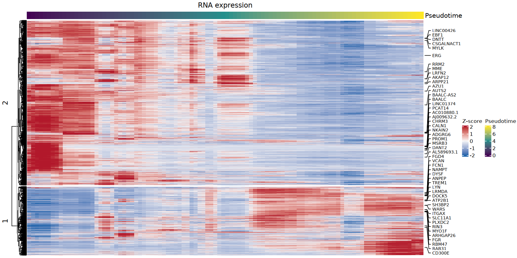
The program uses the plot_complex_heatmap function to generate three types of heatmap objects, then safely outputs them to files via the safe_draw_heatmap function:

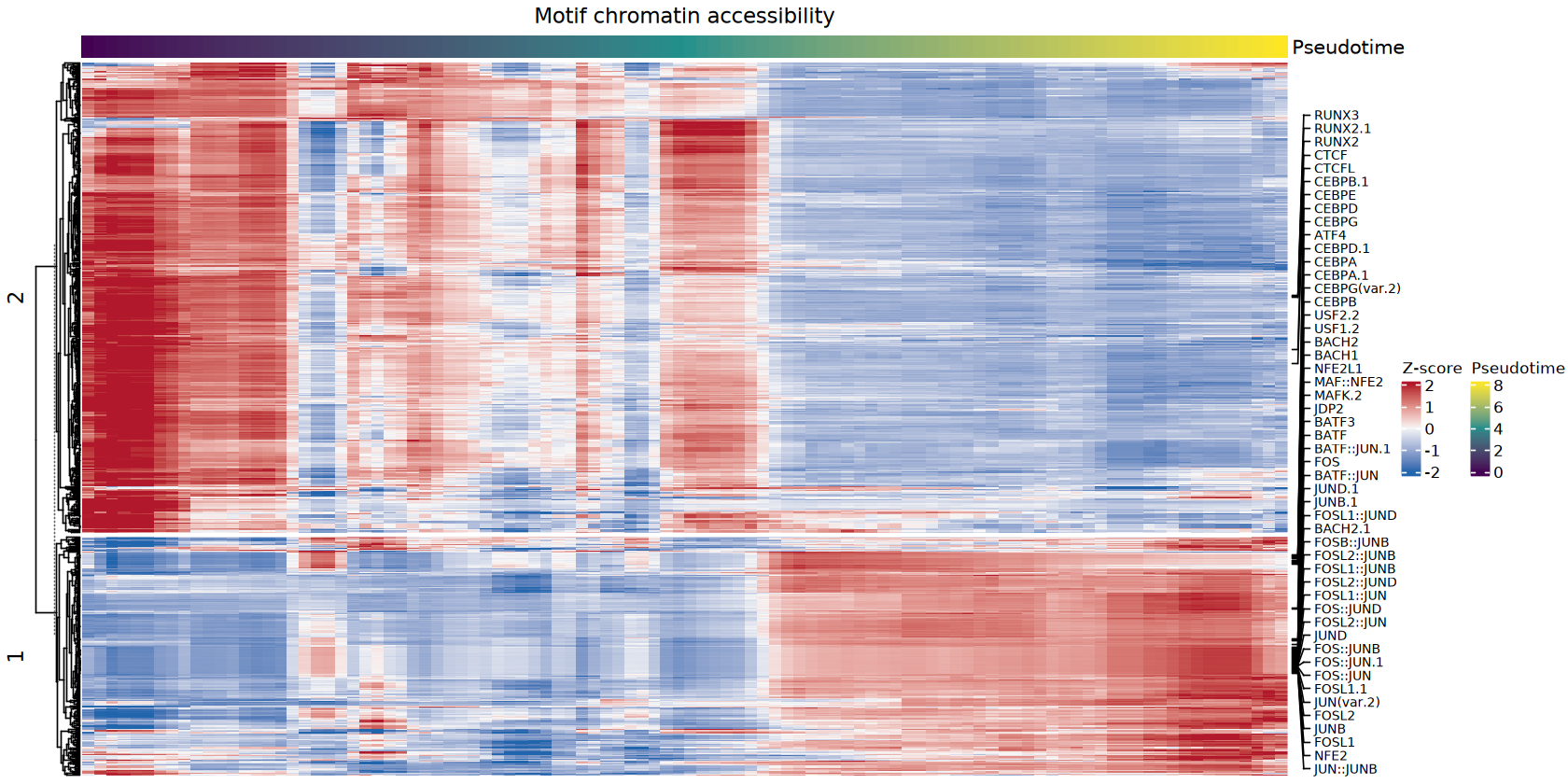
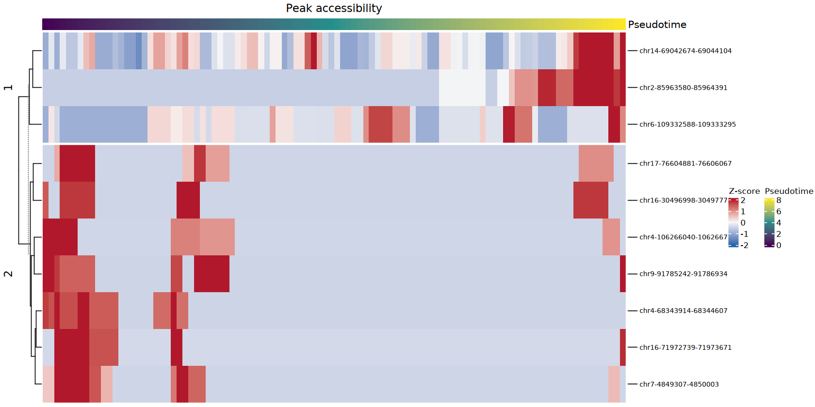
• plot_complex_heatmap Function: Constructs a ComplexHeatmap object with pseudotime color bar annotation and feature labels. Heatmap rows are automatically clustered into 2 groups, corresponding respectively to the two dynamic patterns of rising and falling along pseudotime. Top 50 feature names are annotated on the right using anno_mark, facilitating identification of key molecules.
• safe_draw_heatmap Function: Wraps a tryCatch exception handling mechanism, ensuring the heatmap is stably output in both PNG (300 DPI high-resolution bitmap) and PDF (vector graphics) formats. Even if one format fails to generate, it will not interrupt the overall analysis pipeline.

Three heatmap files are finally generated:

• trajectory_rna_heatmap.png/pdf: Dynamic changes in gene expression along pseudotime.
• trajectory_motif_heatmap.png/pdf: Dynamic changes in Motif chromatin accessibility along pseudotime.
• trajectory_peak_heatmap.png/pdf: Dynamic changes in Peak accessibility along pseudotime.

# Generate consistent colors for cell types
unique_cell_types <- sort(unique(as.character(cell_types)))
unique_cell_types <- unique_cell_types[!is.na(unique_cell_types) & nzchar(unique_cell_types)]
n_colors <- length(unique_cell_types)
if (n_colors == 0) {
  stop("No valid cell types found for heatmap annotation.")
}
ct_colors <- rep(my36colors, length.out = n_colors)
names(ct_colors) <- unique_cell_types

ht_rna <- plot_complex_heatmap(z_rna_obj, "RNA expression", top_rna_labels)
ht_motif <- plot_complex_heatmap(z_motif_obj, "Motif chromatin accessibility", top_motif_labels, motif_name_map)
ht_peak <- plot_complex_heatmap(z_peak_obj, "Peak accessibility", top_atac_labels)

safe_draw_heatmap <- function(ht_obj, file_prefix, width = 12, height = 8, outdir = outdir) {
  pdf_file <- file.path(outdir, paste0(file_prefix, ".pdf"))
  tryCatch({
    pdf(pdf_file, width = width, height = height)
    draw(ht_obj, ht_gap = unit(1, "cm"))
    dev.off()
    print(draw(ht_obj, ht_gap = unit(1, "cm")))  
    #message("Successfully generated: ", pdf_file)
  }, error = function(e) {
    if (names(dev.cur()) != "null device") dev.off()
    warning("Failed to generate PDF for ", file_prefix, ". Reason: ", e$message)
  })
}
# RNA Panel
if (exists("ht_rna")) {
  safe_draw_heatmap(ht_rna, "trajectory_rna_heatmap", outdir = outdir)
} else {
  warning("ht_rna object does not exist. Skipping RNA heatmap.")
}

# Motif Panel
if (exists("ht_motif")) {
  safe_draw_heatmap(ht_motif, "trajectory_motif_heatmap", outdir = outdir)
} else {
  warning("ht_motif object does not exist. Skipping Motif heatmap.")
}

# Peak Panel
if (exists("ht_peak")) {
  safe_draw_heatmap(ht_peak, "trajectory_peak_heatmap", outdir = outdir)
} else {
  warning("ht_peak object does not exist. Skipping Peak heatmap.")
}

💡 Interpretation Guide

Global Description: The heatmap displays Z-score normalized expression/activity changes of all significant features along pseudotime; rows represent features, columns represent pseudotime progress (left to right).

• Color Mapping: Red indicates high expression/high activity, blue indicates low expression/low activity, white indicates moderate levels.
• Top Annotation Bar: Shows the pseudotime gradient process from start (purple) to end (yellow).
• Row Clustering: The heatmap automatically partitions features into two clusters — the upper cluster typically rises along pseudotime (late activation), the lower cluster falls along pseudotime (early programs that exit).
• Right-Side Labels: Annotates the names of Top 50 features with the largest change magnitude, facilitating rapid identification of key regulators.

6.3 Top 10 Feature Scatter Plots

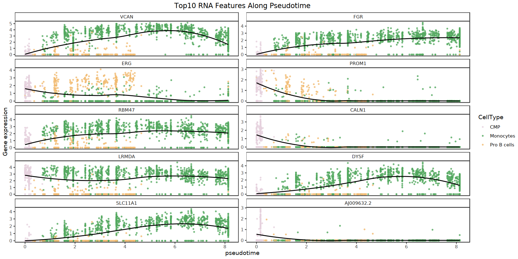
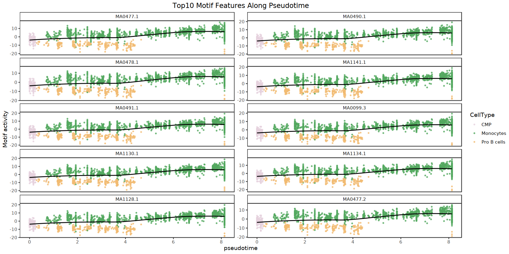
To observe the dynamic change patterns of individual features in more detail, the program further extracts the Top 10 most significantly changing features from each feature type and plots scatter plots along pseudotime:

• Feature Selection:
  • RNA: Top 10 genes by Moran's I in descending order.
  • Motif: Top 10 Motifs by absolute regression estimate in descending order.
  • Peak: Top 10 Peaks by absolute regression estimate in descending order.
• Scatter Plot Drawing: Use the plot_top_feature_scatter function, with pseudotime as the x-axis and feature value as the y-axis; each point represents a cell, colored by cell type. A black LOESS smoothed curve is overlaid to display the overall trend.
• Faceted Display: Each feature has its own small panel, arranged in 2 columns for individual inspection.
• Result Output: Scatter plots for the three feature types are saved respectively as:
  • top10_rna_scatter_pseudotime.png/pdf
  • top10_motif_scatter_pseudotime.png/pdf
  • top10_peak_scatter_pseudotime.png/pdf

# ---- Cell 13.5: top10 feature scatter plots along pseudotime ----
top10_rna <- rownames(head(significant_genes[order(-significant_genes$morans_I), ], 10))
top10_motif <- significant_motifs$id[order(-abs(significant_motifs$estimate))][1:min(10, nrow(significant_motifs))]
top10_peak <- significant_sites[[peak_feature_col]][order(-abs(significant_sites$estimate))][1:min(10, nrow(significant_sites))]

plot_top_feature_scatter(
  mat = rna_mat,
  features = top10_rna,
  pseudotime_vec = pseudotime_vec,
  cell_types = cell_types,
  ct_colors = ct_colors,
  title_prefix = "Top10 RNA Features Along Pseudotime",
  y_label = "Gene expression",
  out_prefix = "top10_rna_scatter_pseudotime",
  outdir = outdir
)

output

\`geom_smooth()\` using formula = 'y ~ x'
\`geom_smooth()\` using formula = 'y ~ x'
\`geom_smooth()\` using formula = 'y ~ x'

plot_top_feature_scatter(
  mat = motif_mat,
  features = top10_motif,
  pseudotime_vec = pseudotime_vec,
  cell_types = cell_types,
  ct_colors = ct_colors,
  title_prefix = "Top10 Motif Features Along Pseudotime",
  y_label = "Motif activity",
  out_prefix = "top10_motif_scatter_pseudotime",
  outdir = outdir
)

output

\`geom_smooth()\` using formula = 'y ~ x'
\`geom_smooth()\` using formula = 'y ~ x'
\`geom_smooth()\` using formula = 'y ~ x'

plot_top_feature_scatter(
  mat = atac_mat,
  features = top10_peak,
  pseudotime_vec = pseudotime_vec,
  cell_types = cell_types,
  ct_colors = ct_colors,
  title_prefix = "Top10 Peak Features Along Pseudotime",
  y_label = "Peak accessibility",
  out_prefix = "top10_peak_scatter_pseudotime",
  outdir = outdir
)

output

\`geom_smooth()\` using formula = 'y ~ x'
\`geom_smooth()\` using formula = 'y ~ x'
\`geom_smooth()\` using formula = 'y ~ x'

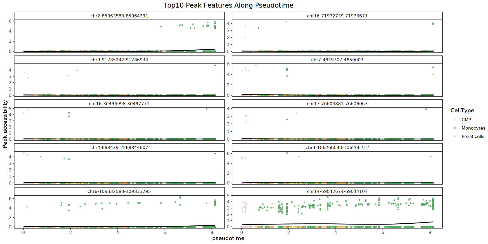
💡 Interpretation Guide

Global Description: The scatter plots display the continuous change of Top 10 features along pseudotime; each panel corresponds to one feature.

• X-axis (pseudotime): Represents the trajectory progress of cells from start to end; further right indicates closer to the terminal state.
• Y-axis: Corresponds to the feature's expression/activity/accessibility value.
• Scatter Point Colors: Colored by cell type, facilitating observation of the distribution positions of different cell types along the trajectory.
• Black Smoothed Curve: LOESS-fitted trend line, intuitively displaying the overall change direction of the feature — rising, falling, or rising then falling.
• Application Scenarios: By observing the curve's shape and steepness, one can determine whether the feature is early-activated, late-activated, or transiently expressed, providing clues for subsequent functional validation.

6.4 TF Specificity Analysis: Focusing on Transcription Factor Dynamics

After completing gene-level differential expression analysis, to further focus on upstream regulators, the program specifically filters transcription factors (TFs) from significantly differentially expressed genes and performs independent visualization analysis.

• TF Name List Construction: Extract all known TF names from the Motif annotation of the Seurat object. For heterodimers (e.g., FOS::JUN), split by :: into independent TF names (FOS and JUN), and remove version labels (e.g., (var.2)) and leading/trailing spaces, ensuring clean and accurate name matching.
• TF Selection: Perform case-insensitive matching between the gene names of significantly differentially expressed genes and the TF name list, filtering out the subset that are transcription factors (significant_tfs). These TFs represent potential upstream regulators whose expression levels change significantly during cell differentiation.
• Result Export: Save the filtered TF list as pseudotime_differentially_expressed_TFs.csv, containing statistical information such as Moran's I, P-value, q-value for each TF, facilitating subsequent functional validation or literature search.
• TF Expression Heatmap: Using the same smoothed matrix construction pipeline as the RNA heatmap, specifically plot an expression heatmap along pseudotime for all significant TFs. The heatmap is output as trajectory_tf_expression_heatmap.png/pdf, with row labels annotating the Top 50 TF names with the most significant changes, intuitively displaying the expression dynamics of transcription factors during the differentiation process.

if (!is.null(motif_obj)) {
  motif_names_raw <- unlist(motif_obj@motif.names)
  # Split heterodimers like FOS::JUN and remove version tags like (var.2)
  tf_names_clean <- unique(unlist(strsplit(motif_names_raw, "::")))
  tf_names_clean <- gsub("\\(var\\.[0-9]+\\)", "", tf_names_clean)
  tf_names_clean <- trimws(tf_names_clean)
  
  # Filter significant genes to only include TFs
  rna_genes <- rownames(significant_genes)
  is_tf <- toupper(rna_genes) %in% toupper(tf_names_clean)
  significant_tfs <- significant_genes[is_tf, , drop = FALSE]
  
  write.csv(
    as.data.frame(significant_tfs),
    file.path(outdir, "pseudotime_differentially_expressed_TFs.csv"),
    row.names = FALSE
  )
      
  # Plot TF heatmap
  if (nrow(significant_tfs) > 0) {
    all_sig_tfs <- rownames(significant_tfs)
    # Select top TFs for labeling
    top_tf_labels <- rownames(head(significant_tfs[order(-significant_tfs$morans_I), ], top_n_heatmap / 2))
    
    z_tf_obj <- build_smoothed_matrix(rna_mat, pseudotime_vec, all_sig_tfs, n_points = 100)
    
    if (!is.null(z_tf_obj)) {
      ht_tf <- plot_complex_heatmap(z_tf_obj, "TF RNA expression", top_tf_labels)
      pdf(file.path(outdir, "trajectory_tf_expression_heatmap.pdf"), width = 8, height = 8)
      draw(ht_tf)
      dev.off()
      draw(ht_tf)        
    }
  }
}

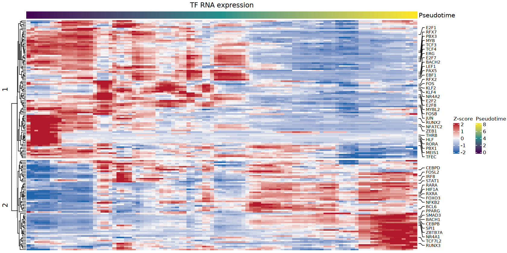
💡 Interpretation Guide

Global Description: The TF-specificity heatmap focuses on the special category of transcription factors, helping researchers quickly locate upstream regulators potentially driving cell fate decisions.

• Filtering Logic: Only genes satisfying both conditions appear in this heatmap: (1) significantly differentially expressed along pseudotime at the RNA level; (2) the gene name exists in the known transcription factor database.
• Biological Significance: If a TF's expression changes significantly along pseudotime, it suggests it may play stage-specific regulatory roles during differentiation — TFs highly expressed early may initiate differentiation programs, while TFs highly expressed late may maintain the terminal state.
• Distinction from Motif Heatmap: The Motif heatmap reflects TF binding activity at the chromatin level (inferred by chromVAR), while the TF heatmap reflects the TF's own expression level at the RNA level. Combining the two can determine: whether the change in TF expression is consistent with the change in its binding activity, thereby inferring whether regulation occurs at the transcriptional or post-translational level.