ATAC + RNA Multi-omics: Basic Analysis Based on ArchR

Author: SeekGene

Time: 24 min

Words: 4.7k words

Updated: 2026-07-07

Reads: 0 times

1. Tutorial Overview

This tutorial leverages the ArchR analysis framework to perform data import and preprocessing, multi-sample joint analysis, dimensionality reduction and clustering, and cell-type annotation on SeekArc single-cell multi-omics data (RNA + ATAC).

This pipeline is intended for SeekArc data where the same cell simultaneously obtains transcriptomic expression and chromatin accessibility: it uses ATAC fragments to build Arrow projects, mounts the seekARC gene expression matrix onto the ArchRProject, and completes the entire workflow — from annotation preparation, quality control, and filtering through joint analysis and regulatory mechanism dissection — in multi-sample scenarios, achieving the following core analytical objectives:

• Multi-Sample Multi-Omics Joint Analysis: Within the same sample or across multiple SeekArc samples, simultaneously leverage RNA expression and ATAC open-chromatin information to more comprehensively characterize cellular states and biological heterogeneity.
• Data Import and Preprocessing: Build gene coordinate annotation based on GTF; read RNA from filtered_feature_bc_matrix and integrate it into a SummarizedExperiment; create Arrow files from fragments (containing Tile Matrix and Gene Score Matrix); initialize ArchRProject and complete RNA/ATAC barcode matching and gene expression matrix mounting, providing a unified project object for subsequent analyses.
• Data Quality Control and Filtering: Perform quality control on ATAC cells based on metrics such as TSS enrichment and fragment count, combined with a stringent matching strategy during RNA mounting, retaining reliable cells consistent across both modalities.
• Single-Modality and Multi-Modality Clustering Analysis: Perform dimensionality reduction and clustering separately based on peak accessibility (ATAC) and Gene Expression (RNA), and integrate both modalities through ArchR's joint dimensionality reduction strategy to compare cell grouping results across different modalities.
• Joint Dimensionality Reduction and Visualization: Fuse RNA and ATAC information to construct a more stable low-dimensional representation, and display cell distribution and inter-sample integration effects via UMAP.
• Cell-Type Annotation: Provide biological interpretation and cell-type labeling of clustering results by combining marker gene expression and genomic accessibility patterns.

library(ArchR)
library(rtracklayer)
library(GenomicFeatures)
library(dplyr)
library(DropletUtils)
library(SummarizedExperiment)

2. Input File Preparation

Input File Requirements

Please ensure that each sample is organized according to a unified directory structure. Each sample should be placed in its own folder; the folder name is recommended to be the sample ID directly, e.g., pbmc_1, pbmc_2, etc. Each sample directory should contain the following:

• filtered_feature_bc_matrix: scRNA-seq expression matrix directory, containing barcodes.tsv.gz, features.tsv.gz, and matrix.mtx.gz.
• filtered_peaks_bc_matrix: scATAC-seq peak accessibility matrix directory, containing barcodes.tsv.gz, features.tsv.gz, and matrix.mtx.gz.
• {sampleID}_A_fragments.tsv.gz: ATAC fragment file, used for downstream construction of ChromatinAssay, computation of TSS enrichment, nucleosome signal, and related analyses.
• {sampleID}_A_fragments.tsv.gz.tbi: Index file corresponding to the ATAC fragment file.
• genes.gtf: Reference genome annotation file, consistent with the genome version used for alignment.

Example Directory Structure

pbmc_1/
├── filtered_feature_bc_matrix/
│   ├── barcodes.tsv.gz
│   ├── features.tsv.gz
│   └── matrix.mtx.gz
├── filtered_peaks_bc_matrix/
│   ├── barcodes.tsv.gz
│   ├── features.tsv.gz
│   └── matrix.mtx.gz
├── pbmc_1_A_fragments.tsv.gz
└── pbmc_1_A_fragments.tsv.gz.tbi

pbmc_2/
├── filtered_feature_bc_matrix/
│   ├── barcodes.tsv.gz
│   ├── features.tsv.gz
│   └── matrix.mtx.gz
├── filtered_peaks_bc_matrix/
│   ├── barcodes.tsv.gz
│   ├── features.tsv.gz
│   └── matrix.mtx.gz
├── pbmc_2_A_fragments.tsv.gz
└── pbmc_2_A_fragments.tsv.gz.tbi

addArchRGenome("hg38") # Select according to your own species information
samples = c('pbmc_1', 'pbmc_2')
rna_dirs <- c(
  "pbmc_1" = "/path/to/pbmc_1/filtered_feature_bc_matrix",
  "pbmc_2" = "/path/to/pbmc_2/filtered_feature_bc_matrix"
)

frag_files <- c(
  "pbmc_1" = "/path/to/pbmc_1/pbmc_1_A_fragments.tsv.gz",
  "pbmc_2" = "/path/to/pbmc_2/pbmc_2_A_fragments.tsv.gz"
)
gtf_file <- "/path/to/genes.gtf"   # genes.gtf annotation file from the human reference genome

3. Data Loading and Preprocessing

This part builds the initial analysis objects from ATAC fragment files and RNA matrix files, providing the data structure foundation for multi-omics integration.

3.1 Initializing ArchRProject

First, use the ATAC fragment files to construct ArchR's dedicated Arrow file format, which is the standard input format for ArchR to process ATAC data. The createArrowFiles function generates Arrow files from each sample's fragment file, containing the genomic tile matrix and gene score matrix. Subsequently, initialize the project object via the ArchRProject function, establishing the container for subsequent analyses.

# --------------------------
# 4. 构建 ArchR 项目
# --------------------------
ArrowFiles <- createArrowFiles(
  inputFiles = frag_files,
  sampleNames = names(frag_files),
  minTSS = 1,
  minFrags = 200,
  addTileMat = TRUE,
  addGeneScoreMat = TRUE
)

projMulti <- ArchRProject(ArrowFiles = ArrowFiles, outputDirectory = "Save-ProjMulti", copyArrows = TRUE)

💡 NoteNote: By default, ArchR filters out cells with TSS enrichment score below 4 and unique alignment count below 1000 (i.e., retaining cells with TSS enrichment score ≥ 4 and unique alignment count ≥ 1000). In practice, it is recommended to reasonably set the minTSS and minFrags parameters to adjust the filtering criteria based on the actual distribution of the data. Creating Arrow files generates a QualityControl directory in the current directory, which includes 2 sample-related quality control plots. The first plot shows a scatter plot of log10(unique nuclear fragments) versus TSS enrichment score, with dashed lines indicating the filtering thresholds. The second plot shows the fragment size distribution.

3.2 Constructing the SummarizedExperiment Object

Since RNA and ATAC matrices are separated in seekARC data, and ArchR's import10xFeatureMatrix function only supports the multi-modal integrated file format output by Cell Ranger ARC, we need to manually construct the SummarizedExperiment object for RNA data. The core steps include: extracting gene coordinate information from the GTF file, reading the RNA expression matrix, matching gene coordinates and filtering out genes without positional information, converting row names to unique gene symbols, and finally generating a data structure compatible with ArchR's addGeneExpressionMatrix function.

gtf <- rtracklayer::import(gtf_file)
genes_gtf <- gtf[gtf$type == "gene"]
gene_id_name <- unique(data.frame(
  gene_id = genes_gtf$gene_id,
  gene_name = genes_gtf$gene_name,
  stringsAsFactors = FALSE
))

txdb <- makeTxDbFromGFF(gtf_file, format = "gtf", organism = "Mus musculus", taxonomyId = 10090)
genes_gr <- genes(txdb)
gene_ids <- mcols(genes_gr)$gene_id
names(genes_gr) <- gene_ids

load_rna_se <- function(sample_id) { 
  sce <- read10xCounts(rna_dirs[[sample_id]], col.names = TRUE) 
  rowData(sce)$gene_id <- rowData(sce)$ID 
  rowData(sce)$gene_name <- rowData(sce)$Symbol 
  
  se <- SummarizedExperiment( 
    assays = list(counts = counts(sce)), 
    rowData = rowData(sce), 
    colData = colData(sce) 
  ) 
  rownames(se) <- rowData(se)$gene_id 
  
  keep <- rowData(se)$gene_id %in% names(genes_gr) 
  if (any(!keep)) { 
    message(sprintf("Sample %s has %d genes lacking gene coordinates.", sample_id, sum(!keep))) 
  } 
  se <- se[keep, ] 
  
  matched_gene_ids <- rowData(se)$gene_id 
  gr <- genes_gr[matched_gene_ids] 
  matched_gene_names <- gene_id_name$gene_name[match(matched_gene_ids, gene_id_name$gene_id)] 
  mcols(gr)$gene_name <- matched_gene_names 
  
  rowRanges(se) <- gr 
  rowData(se)$symbol <- matched_gene_names 
  colnames(se) <- paste(sample_id, colnames(se), sep = "#") 
  
  rownames(se) <- make.unique(rowData(se)$symbol)
  
  rm(sce) 
  gc() 
  se 
}

RNA_list <- lapply(samples, load_rna_se)
se_combined <- do.call(cbind, RNA_list)

3.3 Adding RNA's SummarizedExperiment to ArchRProject

By matching the shared barcodes between ATAC and RNA data, filter to retain cells common to both modalities. Use the addGeneExpressionMatrix function to integrate the RNA expression matrix into the ArchRProject, creating the gene expression matrix, enabling joint storage of RNA and ATAC data, and establishing the foundation for subsequent multi-modal joint analysis.

common_cells <- intersect(getCellNames(projMulti), colnames(se_combined))


if (length(common_cells) == 0) {
  stop("No cells could be matched simultaneously. Please check the barcode format or whitelist.")
}

projMulti <- subsetArchRProject(
  ArchRProj = projMulti,
  cells = common_cells,
  outputDirectory = "Save-ProjMulti2",
  force = TRUE
)

se_combined <- se_combined[, common_cells, drop = FALSE]

projMulti <- addGeneExpressionMatrix(
  input = projMulti,
  seRNA = se_combined,
  strictMatch = TRUE,
  force = TRUE
)

4. Data Quality Control

4.1 Quality Metrics

After completing data reading and project initialization, comprehensive quality control must be performed on each cell to remove low-quality cells and ensure the reliability of subsequent analyses. ArchR automatically computes various quality metrics during Arrow file construction, covering both ATAC and RNA modalities.

RNA Quality Metrics:

• Gex_nUMI: Total RNA molecules (total UMI count) detected in each cell, reflecting sequencing depth. Too low may indicate low cell capture efficiency; too high may suggest doublets.
• Gex_nGenes: Number of unique genes detected in each cell, reflecting transcriptome complexity. Too low is usually accompanied by high mitochondrial proportion, indicating low-quality cells; too high may suggest doublets.
• Gex_MitoRatio: Mitochondrial gene expression proportion, used to assess cell status. Normal cells typically have < 0.2; too high (> 0.2–0.3) may indicate damaged or low-quality cells.

ATAC Quality Metrics:

• TSSEnrichment: Transcription start site enrichment score, evaluating the degree to which open-chromatin signal is enriched in gene promoter regions. High values indicate good data quality; typically > 2 is acceptable, > 4 is high quality.
• nFrags: Total ATAC fragments per cell, measuring the strength of chromatin accessibility signal. Too low indicates insufficient sequencing coverage; too high may suggest multiple captures or doublets.
• NucleosomeRatio: Nucleosome signal ratio, reflecting fragment length distribution characteristics. Normal cells typically have < 2; too high (> 4) may indicate apoptotic or low-quality cells.

plotQC <- plotGroups(
  ArchRProj = projMulti,
  groupBy = "Sample",
  colorBy = "cellColData",
  name = c("TSSEnrichment", "nFrags", "NucleosomeRatio"),
  alpha = 0.4,
  plotAs = "violin"
)

plotQC_RNA <- plotGroups(
  ArchRProj = projMulti,
  groupBy = "Sample",
  colorBy = "cellColData",
  name = c("Gex_nUMI", "Gex_MitoRatio","Gex_nGenes"),
  alpha = 0.4,
  plotAs = "violin"
)

plotQC$`nFrags`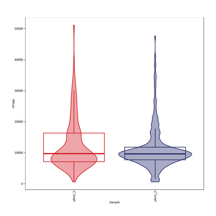

plotQC$NucleosomeRatio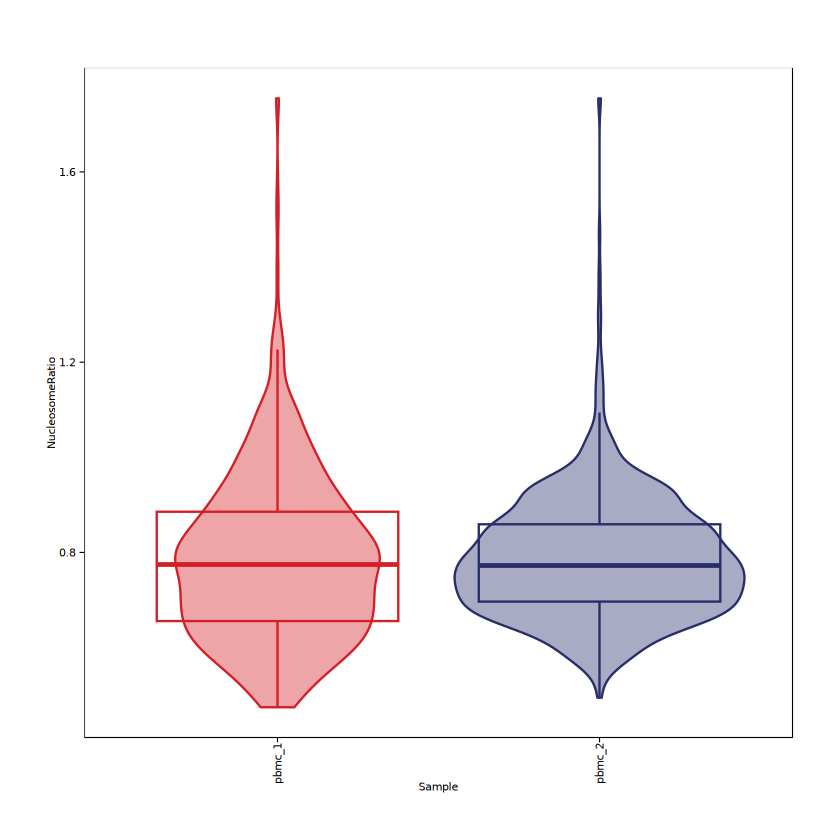

plotQC$TSSEnrichment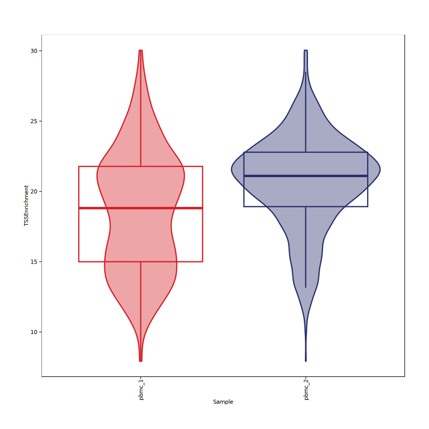

plotQC_RNA$Gex_MitoRatio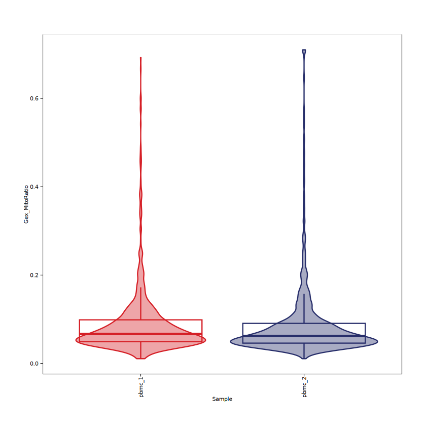

plotQC_RNA$Gex_nUMI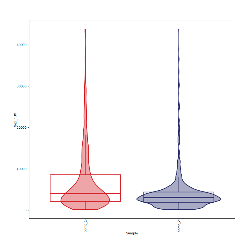

plotQC_RNA$Gex_nGenes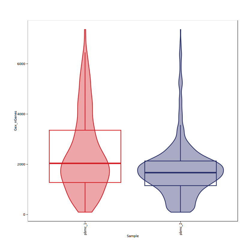

Note It is recommended to focus on the following:

• Whether there are obvious outliers, long-tailed distributions, or bimodal distributions: In the visualization of quality metrics, check for outlier cells with extreme high or low values, which may represent low-quality cells, doublets, or technical artifacts. Long-tailed or bimodal distributions may indicate the presence of cell subpopulations in different states within the sample.
• Whether the distribution of quality metrics is consistent across different samples: Compare the distribution differences across samples in key quality metrics (e.g., TSS enrichment score, fragment count, mitochondrial proportion, etc.). Significant batch differences may require batch correction before dimensionality reduction.
• Reasonably adjust filtering thresholds based on visualization results: Avoid using fixed absolute thresholds; instead, set filtering criteria based on the actual data distribution, retaining enough cells while removing obvious low-quality cells, to improve the clarity and reliability of downstream clustering and UMAP visualization.

4.2 Filtering Out Low-Quality Cells

Based on the quality metrics shown in the preceding violin plots, filter out low-quality cells to remove abnormal cells and improve the reliability of downstream analysis results. Specific filtering thresholds should be set according to the actual sample conditions, typically guided by the violin plots and scatter plots of the quality metrics.

projMulti_filtered <- subsetArchRProject(
  ArchRProj = projMulti,
  cells = getCellNames(projMulti)[
    projMulti$TSSEnrichment > 1 &
    projMulti$nFrags > 500 &
    projMulti$nFrags < 50000 &
    projMulti$NucleosomeRatio < 1 &
    projMulti$Gex_nUMI > 500 &
    projMulti$Gex_nUMI < 30000 &
    projMulti$Gex_nGenes > 200 &
    projMulti$Gex_nGenes < 8000 &
    projMulti$Gex_MitoRatio < 0.20
  ],
  outputDirectory = "Filtered_Project",
  force = TRUE
)

4.3 Doublet Identification

After low-quality cell filtering, ArchR's automated doublet detection and filtering functionality can be used to further remove potential doublets.

• Compute each cell's doublet score using the addDoubletScores() function; this function predicts the likelihood of a cell being a doublet based on its chromatin accessibility features (simulated doublets).
• Filter cells based on the doublet score using the filterDoublets() function. The key filterRatio parameter in the function controls the filtering stringency, defined as: the maximum filtering proportion of predicted doublets computed based on the number of cells passing quality control.

projMulti_filtered <- addDoubletScores(projMulti_filtered, force = TRUE)

projMulti_filtered <- filterDoublets(projMulti_filtered)

5. Linear Dimensionality Reduction Analysis

After constructing the multi-modal data object, perform dimensionality reduction separately on ATAC and RNA data to extract the core data structure and reduce computational dimensions. ArchR employs the iterative Latent Semantic Indexing (LSI) algorithm, which effectively handles high-dimensional sparse chromatin accessibility data and gene expression data.

5.1 Iterative LSI Dimensionality Reduction

For the two data types, different feature selection strategies are adopted:

1. ATAC Data: Build a tile matrix based on 500-bp genome-wide windows, and progressively focus on the most variable chromatin accessibility regions through iterative LSI.
2. RNA Data: Build an expression matrix based on highly variable genes, and identify major transcriptomic patterns through LSI.

5.2 Multi-Modal Data Integration

Integrate the LSI dimensionality reduction results of ATAC and RNA via the addCombinedDims function to generate the joint dimensionality reduction result LSI_Combined, providing a unified foundation for subsequent multi-modal joint analysis.

projMulti_filtered <- addIterativeLSI(
  ArchRProj = projMulti_filtered, 
  clusterParams = list(
    resolution = 0.2, 
    sampleCells = 10000,
    n.start = 10
  ),
  saveIterations = FALSE,
  useMatrix = "TileMatrix", 
  depthCol = "nFrags",
  name = "LSI_ATAC"
)

projMulti_filtered <- addIterativeLSI(
  ArchRProj = projMulti_filtered, 
  clusterParams = list(
    resolution = 0.2, 
    sampleCells = 10000,
    n.start = 10
  ),
  saveIterations = FALSE,
  useMatrix = "GeneExpressionMatrix", 
  depthCol = "Gex_nUMI",
  varFeatures = 2500,
  firstSelection = "variable",
  binarize = FALSE,
  name = "LSI_RNA"
)

projMulti_filtered <- ArchR::addCombinedDims(projMulti_filtered, 
                                             reducedDims = c("LSI_ATAC", "LSI_RNA"),   
                                             name = "LSI_Combined")

6. Nonlinear Dimensionality Reduction and Clustering Analysis

After completing LSI dimensionality reduction and multi-modal integration, we map the high-dimensional data to two-dimensional space through nonlinear dimensionality reduction (UMAP) to visualize the complex relationships between cells. UMAP effectively preserves both local and global structures in high-dimensional space, facilitating intuitive observation of cell subpopulation distribution.

6.1 Three Dimensionality Reduction Strategies

1. Integrated Modality Dimensionality Reduction: Perform UMAP visualization based on the integrated multi-modal LSI results (LSI_Combined), reflecting the joint signal of ATAC and RNA data.
2. ATAC Single-Modality Dimensionality Reduction: Perform UMAP visualization based on pure ATAC LSI results (LSI_ATAC), highlighting chromatin accessibility patterns.
3. RNA Single-Modality Dimensionality Reduction: Perform UMAP visualization based on pure RNA LSI results (LSI_RNA), reflecting gene expression profile similarity.

projMulti_filtered <- addUMAP(projMulti_filtered, reducedDims = "LSI_Combined", name = "UMAP_Combined", minDist = 0.8, force = TRUE)
projMulti_filtered <- addUMAP(projMulti_filtered, reducedDims = "LSI_ATAC", name = "UMAP_ATAC", minDist = 0.8, force = TRUE)
projMulti_filtered <- addUMAP(projMulti_filtered, reducedDims = "LSI_RNA", name = "UMAP_RNA", minDist = 0.8, force = TRUE)
projMulti_filtered <- addClusters(projMulti_filtered, reducedDims = "LSI_Combined", name = "Clusters_Combined", resolution = 0.4, force = TRUE)
projMulti_filtered <- addClusters(projMulti_filtered, reducedDims = "LSI_ATAC", name = "Clusters_ATAC", resolution = 0.4, force = TRUE)
projMulti_filtered <- addClusters(projMulti_filtered, reducedDims = "LSI_RNA", name = "Clusters_RNA", resolution = 0.4, force = TRUE)

Note

Parameter Description

• minDist = 0.8: Controls the minimum distance between points in UMAP; lower values separate tight cell subpopulations, higher values present more continuous cell-state transitions. Typically set to 0.1–0.8.
• resolution = 0.4: Controls clustering granularity; lower values produce coarser clusters (fewer clusters), higher values produce finer subpopulation divisions (typically based on Seurat's FindClusters algorithm).

6.2 Dimensionality Reduction and Clustering Visualization

p1 <- plotEmbedding(projMulti_filtered, name = "Clusters_ATAC", embedding = "UMAP_ATAC", size = 1, labelAsFactors=F, labelMeans=F)
p2 <- plotEmbedding(projMulti_filtered, name = "Clusters_RNA", embedding = "UMAP_RNA", size = 1, labelAsFactors=F, labelMeans=F)
p3 <- plotEmbedding(projMulti_filtered, name = "Clusters_Combined", embedding = "UMAP_Combined", size = 1, labelAsFactors=F, labelMeans=F)

options(repr.plot.width = 14, repr.plot.height = 7)
p1+p2+p3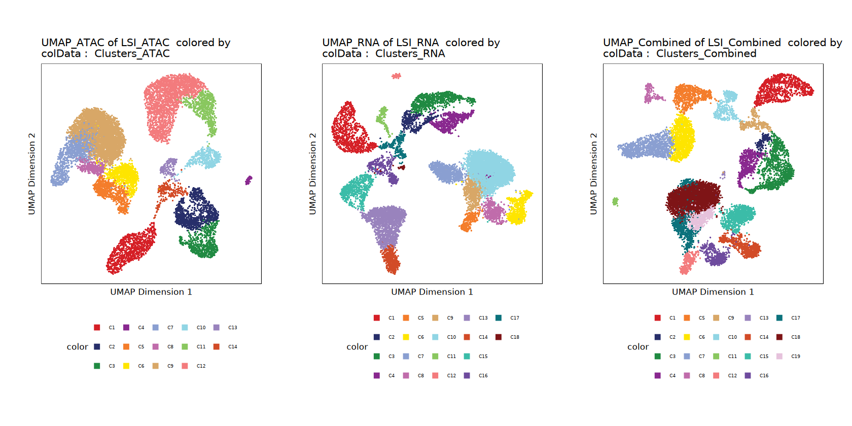

p4 <- plotEmbedding(projMulti_filtered, name = "Sample", embedding = "UMAP_ATAC", size = 1, labelAsFactors=F, labelMeans=F)
p5 <- plotEmbedding(projMulti_filtered, name = "Sample", embedding = "UMAP_RNA", size = 1, labelAsFactors=F, labelMeans=F)
p6 <- plotEmbedding(projMulti_filtered, name = "Sample", embedding = "UMAP_Combined", size = 1, labelAsFactors=F, labelMeans=F)

options(repr.plot.width = 14, repr.plot.height = 7)
p4+p5+p6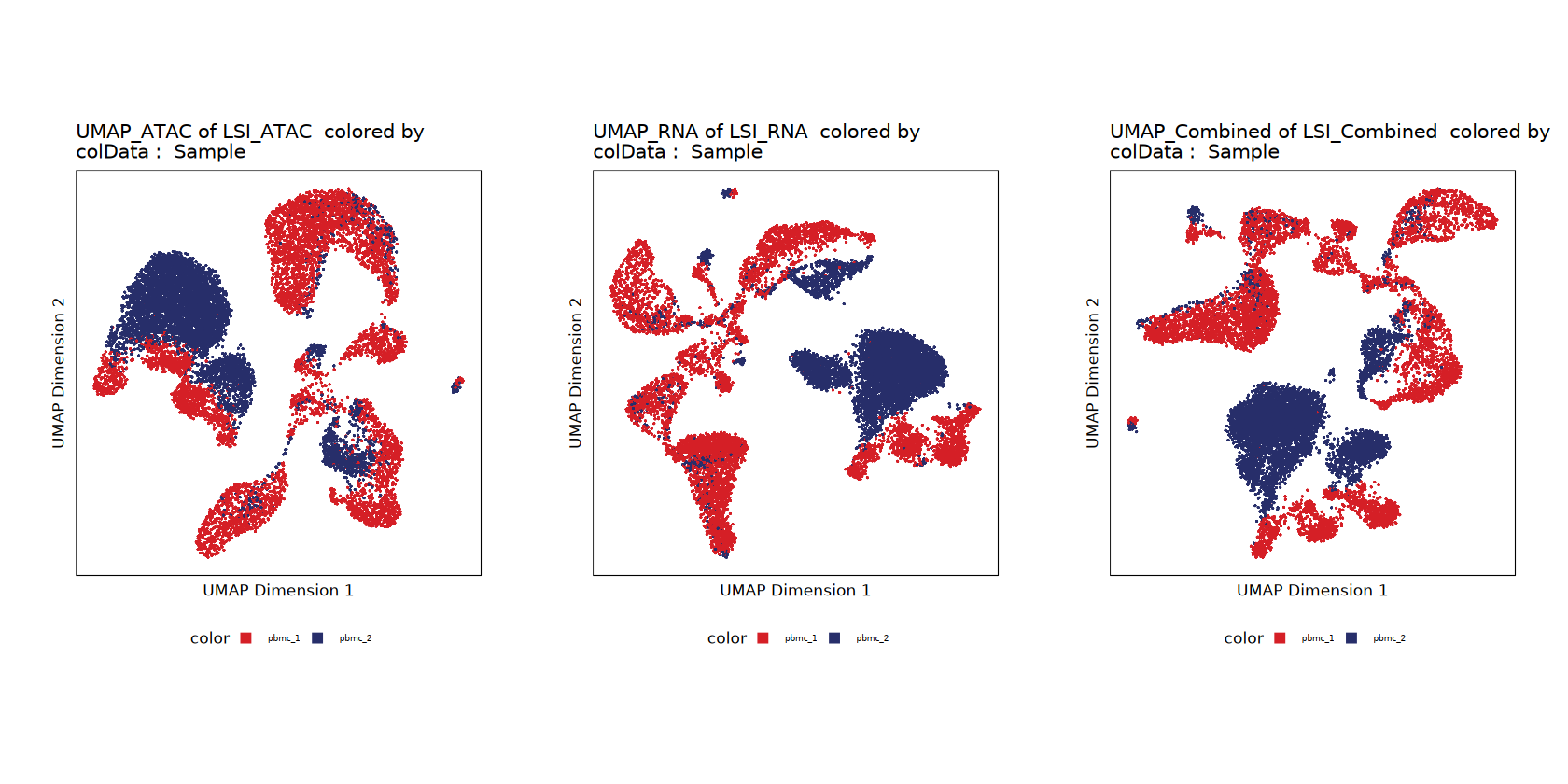

Note Obvious batch separation between samples is observed in UMAP visualization, indicating that although iterative LSI dimensionality reduction can alleviate some batch effects introduced by experimental techniques, its correction ability may be limited for significant inter-sample technical variation. If batch effects still interfere with the interpretation of downstream biological signals, it is recommended to consider applying additionally a dedicated batch correction algorithm (such as Harmony) after LSI dimensionality reduction for further processing.

6.3 Batch Correction of ATAC and RNA Separately Using Harmony

In multi-sample data analysis, if obvious inter-sample batch separation is still observed after LSI dimensionality reduction, an additional batch correction step is needed. ArchR has the Harmony algorithm built in, designed specifically for single-cell data; through iterative clustering and linear correction of principal components, it can effectively integrate data from different samples or experimental batches.

Harmony is invoked in ArchR via the addHarmony() function, where the user needs to specify the groupBy parameter to define the batch variable to be corrected (typically sample origin).

In this analysis, independent Harmony batch correction is performed separately on ATAC and RNA data:

1. ATAC Data Correction: Based on the LSI_ATAC dimensionality reduction results, generate the corrected embedding Harmony_ATAC.
2. RNA Data Correction: Based on the LSI_RNA dimensionality reduction results, generate the corrected embedding Harmony_RNA.

Finally, the two corrected dimensionality reduction results are integrated via addCombinedDims() to generate the joint batch-corrected dimensionality reduction representation LSI_Combined_Harmony, for subsequent multi-modal joint analysis.

projMulti_filtered <- addHarmony(
    ArchRProj = projMulti_filtered,
    reducedDims = "LSI_ATAC",
    name = "Harmony_ATAC",
    groupBy = "Sample",
    theta = 5, 
    sigma = 0.01,
    force = TRUE
)


projMulti_filtered <- addHarmony(
    ArchRProj = projMulti_filtered,
    reducedDims = "LSI_RNA",
    name = "Harmony_RNA",
    groupBy = "Sample",
    theta = 5,
    sigma = 0.01,
    force = TRUE
)

projMulti_filtered <- ArchR::addCombinedDims(projMulti_filtered, 
                                             reducedDims = c("Harmony_ATAC", "Harmony_RNA"),   
                                             name = "LSI_Combined_Harmony")

6.4 Dimensionality Reduction and Clustering Based on Batch-Corrected Results

After completing Harmony batch correction, re-execute UMAP nonlinear dimensionality reduction and cell clustering based on the corrected dimensionality reduction results, to evaluate the batch correction effect and obtain more accurate cell groupings.

Dimensionality Reduction and Clustering Strategy

1. ATAC Batch-Corrected Results: Perform UMAP dimensionality reduction and clustering based on Harmony_ATAC, obtaining UMAP_Harmony_ATAC and Clusters_Harmony_ATAC, reflecting chromatin accessibility patterns after batch effect removal.

2. RNA Batch-Corrected Results: Perform UMAP dimensionality reduction and clustering based on Harmony_RNA, obtaining UMAP_Harmony_RNA and Clusters_Harmony_RNA, reflecting transcriptomic features after batch effect removal.

3. Joint Batch-Corrected Results: Perform UMAP dimensionality reduction and clustering based on the integrated LSI_Combined_Harmony, obtaining UMAP_Combined_Harmony and Clusters_Combined_Harmony, comprehensively considering multi-modal information after batch removal.

projMulti_filtered <- addUMAP(projMulti_filtered, reducedDims = "Harmony_ATAC", 
                              name = "UMAP_Harmony_ATAC", minDist = 0.8, force = TRUE)
projMulti_filtered <- addUMAP(projMulti_filtered, reducedDims = "Harmony_RNA", 
                              name = "UMAP_Harmony_RNA", minDist = 0.8, force = TRUE)
projMulti_filtered <- addUMAP(projMulti_filtered, reducedDims = "LSI_Combined_Harmony", 
                              name = "UMAP_Combined_Harmony", minDist = 0.8, force = TRUE)


projMulti_filtered <- addClusters(projMulti_filtered, reducedDims = "Harmony_ATAC", 
                                  name = "Clusters_Harmony_ATAC", resolution = 0.4, force = TRUE)
projMulti_filtered <- addClusters(projMulti_filtered, reducedDims = "Harmony_RNA", 
                                  name = "Clusters_Harmony_RNA", resolution = 0.4, force = TRUE)
projMulti_filtered <- addClusters(projMulti_filtered, reducedDims = "LSI_Combined_Harmony", 
                                  name = "Clusters_Combined_Harmony", resolution = 0.4, force = TRUE)

p7 <- plotEmbedding(projMulti_filtered, name = "Sample", embedding = "UMAP_Harmony_ATAC", size = 1, labelAsFactors=F, labelMeans=F)
p8 <- plotEmbedding(projMulti_filtered, name = "Sample", embedding = "UMAP_Harmony_RNA", size = 1, labelAsFactors=F, labelMeans=F)
p9 <- plotEmbedding(projMulti_filtered, name = "Sample", embedding = "UMAP_Combined_Harmony", size = 1, labelAsFactors=F, labelMeans=F)

options(repr.plot.width = 14, repr.plot.height = 7)
p7+p8+p9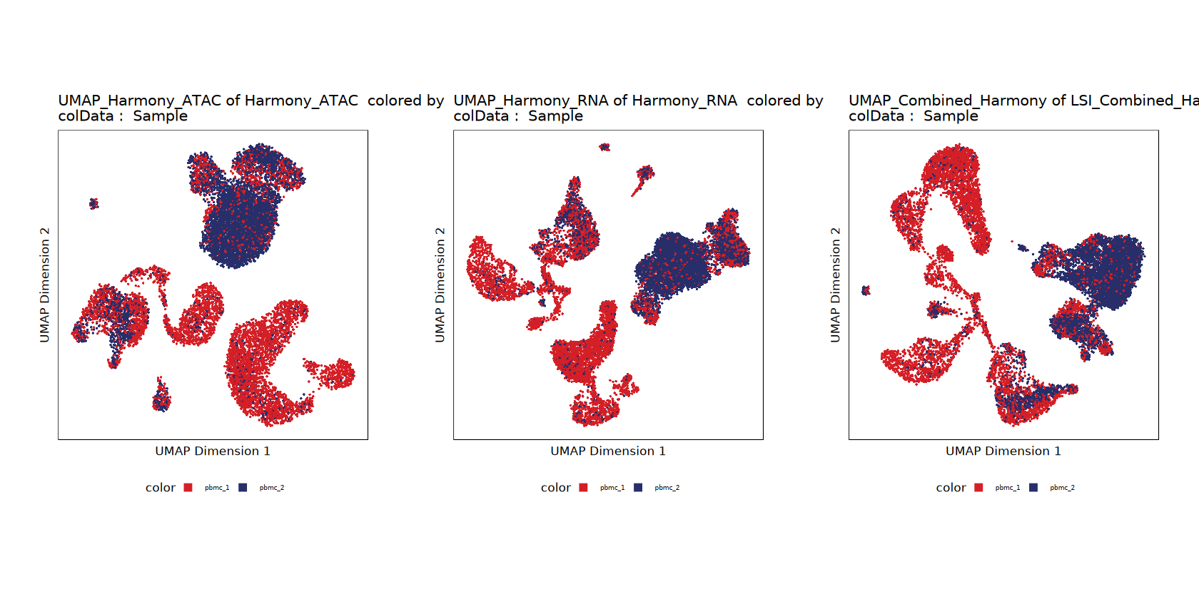

library(cowplot)

sample_list <- unique(projMulti_filtered$Sample)

plot_list <- lapply(sample_list, function(sample_i) {
  plotEmbedding(
    ArchRProj = projMulti_filtered,
    embedding = "UMAP_Combined_Harmony",
    colorBy = "cellColData",
    name = "Clusters_Combined_Harmony",
    highlightCells = getCellNames(projMulti_filtered)[projMulti_filtered$Sample == sample_i],
    pal = c("Non.Highlighted" = "lightgrey"),
    size = 0.8,
    baseSize = 8,
    title = sample_i
  )
})

p_faceted <- plot_grid(plotlist = plot_list, ncol = 3)
print(p_faceted)

Note: Batch Correction Effect Evaluation

Evaluation of batch correction effectiveness needs to be judged based on visualization results:

1. Mixing Check: Compare sample distributions before and after batch correction (UMAP_Combined vs. UMAP_Combined_Harmony); ideally, cells from different samples should mix more uniformly in UMAP space after correction, rather than separating by sample.
2. Biological Signal Retention: Check whether batch correction preserves clear cell-type separation. Over-correction causes blurring of cell subpopulation boundaries, while under-correction fails to effectively integrate samples.
3. Clustering Consistency: Observe whether the same cell type across different samples is assigned to the same cluster, ensuring that batch correction has not introduced new technical bias.
4. Downstream Analysis Selection: If the correction effect is ideal, it is recommended to use the batch-corrected clustering results (e.g., Clusters_Combined_Harmony) for subsequent differential analysis and functional annotation, to obtain more stable and reproducible biological findings.

p10 <- plotEmbedding(projMulti_filtered, name = "Clusters_Harmony_ATAC", embedding = "UMAP_Harmony_ATAC", size = 1, labelAsFactors=F, labelMeans=F)
p11 <- plotEmbedding(projMulti_filtered, name = "Clusters_Harmony_RNA", embedding = "UMAP_Harmony_RNA", size = 1, labelAsFactors=F, labelMeans=F)
p12 <- plotEmbedding(projMulti_filtered, name = "Clusters_Combined_Harmony", embedding = "UMAP_Combined_Harmony", size = 1, labelAsFactors=F, labelMeans=F)

options(repr.plot.width = 14, repr.plot.height = 7)
p10+p11+p12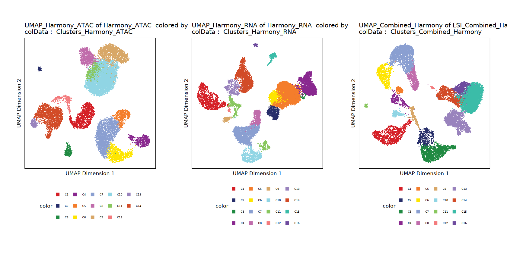

7. Grouped Peak Calling and Matrix Construction

After completing cell clustering (Clusters_Combined_Harmony) analysis, based on cell-type grouping results, we adopt a grouped strategy to re-perform chromatin accessible region (Peak) identification and construct a cell × Peak count matrix, providing high-resolution input for downstream regulatory element analysis.

7.1 Group Coverage Computation

The addGroupCoverages() function merges the ATAC-seq fragments of all cells within the same cluster, based on the specified cell grouping (groupBy = "Clusters_Combined_Harmony"), generating aggregated coverage files for each cell subpopulation. The purpose of this step is to accumulate sufficient signal depth for each cell type, ensuring the sensitivity of downstream Peak Calling, and particularly helping to capture regions with weak but biologically important accessibility in rare cell subpopulations.

addArchRThreads(4)

projMulti_filtered <- addGroupCoverages(ArchRProj = projMulti_filtered, groupBy = "Clusters_Combined_Harmony", verbose = FALSE)

7.2 Grouped Peak Calling

addReproduciblePeakSet() is the core execution step, adopting a group-independent identification strategy:

1. Independent Identification: Run MACS2 independently within each cell subpopulation (specifying the pathToMacs2 path) for Peak Calling, thereby identifying accessible regions specific to that cell type.
2. Merging and Deduplication: Merge the Peak coordinates identified from all subpopulations to generate a non-redundant unified Peak set (Union Peak Set). Compared to calling on the entire dataset at once, this strategy more robustly captures cell-type-specific regulatory elements, avoiding signal dilution or masking.

pathToMacs2 <- "/PROJ/development/changyanxia/software/bin/macs2"
projMulti_filtered <- addReproduciblePeakSet(ArchRProj = projMulti_filtered, groupBy = "Clusters_Combined_Harmony", pathToMacs2 = pathToMacs2)

7.3 Peak Matrix Construction

The addPeakMatrix() function computes fragment counts in these regions for each cell based on the integrated Peak set, constructing the cell × Peak accessibility matrix. This matrix is the core data foundation for subsequent differential Peak analysis, Motif enrichment, Peak-to-Gene association, and other epigenetic analyses.

projMulti_filtered <- addPeakMatrix(ArchRProj = projMulti_filtered)

8. Cell-Type Annotation

8.1 Differential Gene Expression Analysis

Identify genes that are specifically highly expressed in each cell cluster, and screen for representative marker genes based on expression proportion and fold change, providing a preliminary basis for cell-type identification. A heatmap can be used to inspect the expression of Top differentially expressed genes across different clusters, assisting in determining the cell type corresponding to each cluster.

addArchRThreads(threads = 1) 
getAvailableMatrices(projMulti_filtered)
DEG <- getMarkerFeatures(
    ArchRProj = projMulti_filtered,
    groupBy = "Clusters_Combined_Harmony",
    #groupBy = "Clusters_Combined",
    useMatrix = "GeneExpressionMatrix",
    bias = c("TSSEnrichment", "log10(nFrags)", "log10(Gex_nUMI)")  # 包含RNA偏差
)

markerList <- getMarkers(DEG, cutOff = "FDR < 0.05 & Log2FC > 0.5")
#markerList <- markerList[c(1:11,14)]
top_n <- 4
top_markers_list <- lapply(markerList, function(df) {
  df_sorted <- df[order(df$Log2FC, decreasing = TRUE), ]
  return(head(df_sorted, top_n))
})
for(cluster in names(top_markers_list)){
  top_markers_list[[cluster]]$Cluster <- cluster
}
all_top_markers <- do.call(rbind, top_markers_list)

heatmap_plot1 <- plotMarkerHeatmap(
  seMarker = DEG,
  cutOff = "FDR <= 0.1 & Log2FC >= 1",
  binaryClusterRows = TRUE,
  labelMarkers = unique(all_top_markers$name),
  clusterCols = TRUE,
  transpose = FALSE
)

heatmap_plot1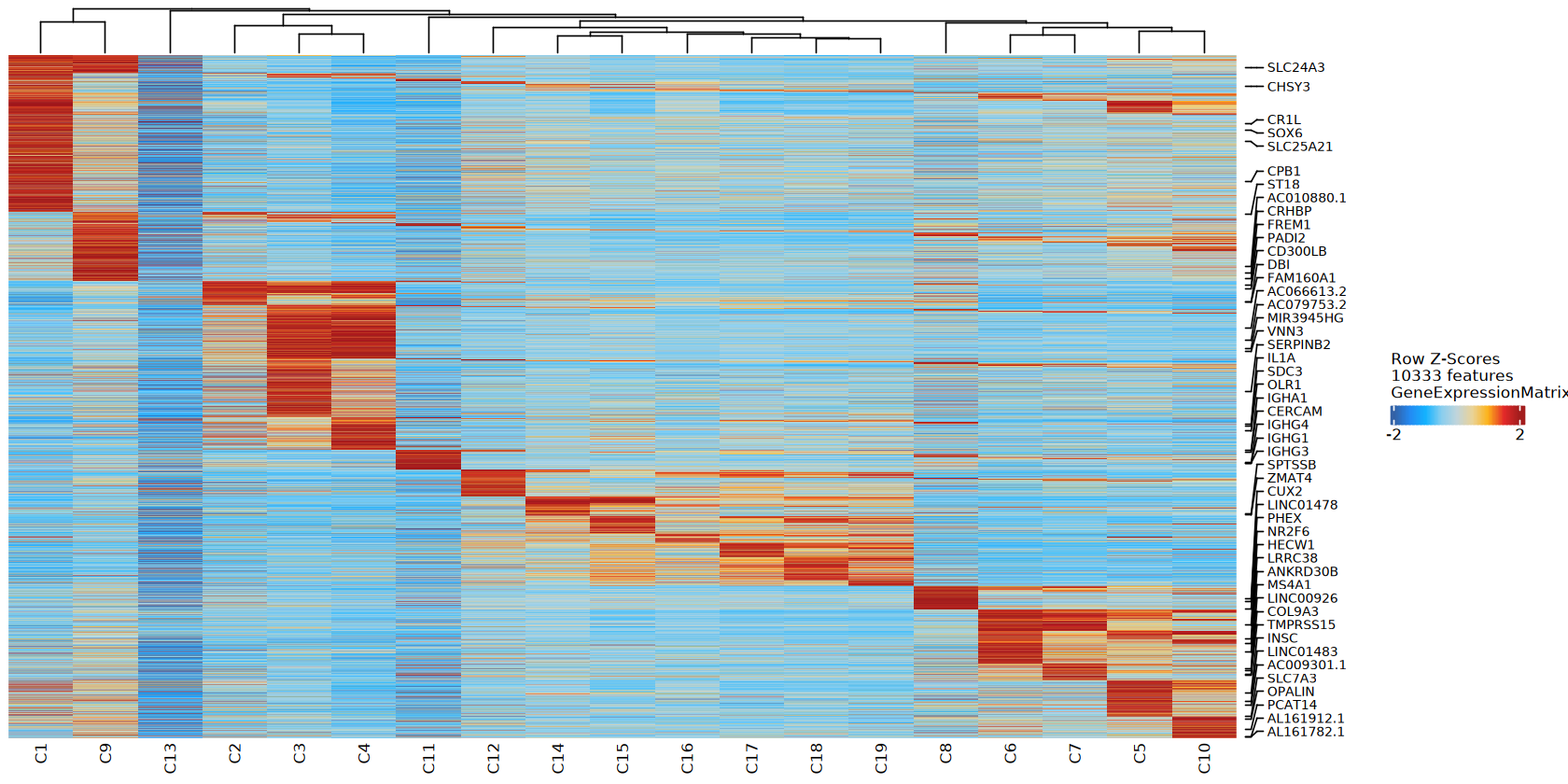

8.2 Inspecting Marker Gene Expression at the scRNA-seq Data Level

The example data in this tutorial are PBMC, so we have compiled common immune cell types and their corresponding marker gene sets. In actual analyses, marker genes should be customized according to sample origin and tissue type. Subsequently, a heatmap can be used to inspect the expression of marker genes across different clusters, assisting in determining the cell type corresponding to each cluster.

pbmc_marker_integrated <- list(
  "Plasma Cells" = c("IGHG1", "IGKC"),
  "Monocytes" = c("VCAN", "FCN1", "TREM1"),
  "B cells" = c("MS4A1", "BACH2", "PAX5"),
  "CMP" = c("MPO"),
  "Pro B cells" = c("DNTT"),
  "Erythroblast" = c("ALAS2", "NFIA", "SOX6"),
  "T cells" = c("PLXNA4", "THEMIS", "ITK", "BCL11B"),
  "NK cells" = c("NCAM1", "KLRC3"),
  "Dividing B cells" = c("MKI67", "TOP2A"),
  "pDC" = c("RUNX2")
)

heatmap_plot <- plotMarkerHeatmap(
  seMarker = DEG,
  cutOff = "FDR <= 0.1 & Log2FC >= 1",
  labelMarkers = unlist(pbmc_marker_integrated),
  binaryClusterRows = TRUE,
  clusterCols = TRUE,
  transpose = FALSE
)

heatmap_plot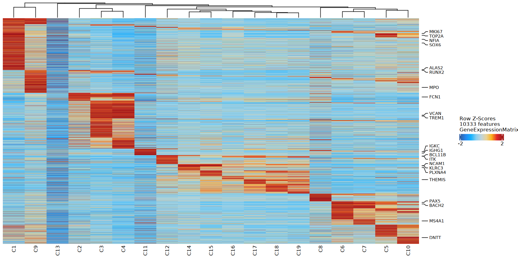

8.3 Inspecting Marker Gene Genomic Region Accessibility at the scATAC-seq Data Level

In addition to RNA expression, the accessibility of regulatory regions around marker genes can also be inspected at the scATAC-seq data level to further assist cell-type annotation. Typically, by combining the peak signal near the gene, the degree of chromatin accessibility, and the accessibility differences between different clusters, one can determine whether a specific marker gene is in an active regulatory state in the corresponding cell population.

my_clusters <- sort(unique(projMulti_filtered$Clusters_Combined_Harmony))

p1 <- plotBrowserTrack(
  ArchRProj = projMulti_filtered,
  geneSymbol  = c("VCAN", "RUNX2", "MPO", "ALAS2", "THEMIS", "KLRC3"),
  groupBy = "Clusters_Combined_Harmony",
  #groupBy = "Clusters_Combined",  
  useGroups = my_clusters,
  tileSize = 100,
  upstream = 5000,
  downstream = 5000,
  title = "VCAN Region"
)

options(repr.plot.width = 16, repr.plot.height = 8)
patchwork::wrap_plots(p1)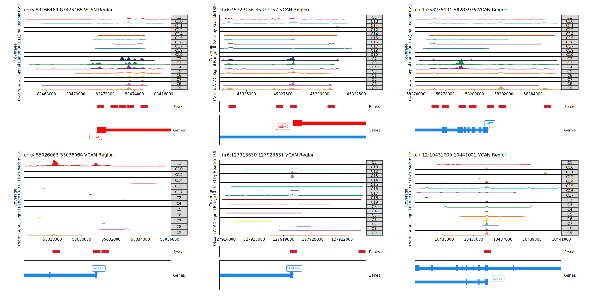

8.4 Cell-Type Labeling and Visualization

Map and write the inferred cell-type names into the ArchRProject via addCellColData, facilitating display in subsequent visualizations and differential analyses directly by biologically meaningful categories (e.g., T cells, B cells).

print(table(projMulti_filtered$UMAP_Combined_Harmony))

celltype_mapping <- c(
  "C1" = "T cells", "C2" = "Monocytes", "C3" = "NK cells",
  "C4" = "Erythroblast", "C5" = "B cells", "C6" = "T cells",
  "C7" = "B cells", "C8" = "Dividing B cells", "C9" = "Pro B cells",
  "C10" = "CMP", "C11" = "T cells", "C12" = "pDC",
  "C13" = "T cells", "C14" = "B cells", "C15" = "Monocytes",
  "C16" = "Plasma Cells", "C17" = "NK cells", "C18" = "NA","C19" = "NA","C20" = "NA"
)

celltype_annotations <- celltype_mapping[as.character(projMulti_filtered$UMAP_Combined_Harmony)]

projMulti_filtered <- addCellColData(
  ArchRProj = projMulti_filtered,
  data = celltype_annotations,
  name = "CellType",
  cells = getCellNames(projMulti_filtered)
)

print(table(projMulti_filtered$CellType))

p1=plotEmbedding(projMulti_filtered, name = "CellType", embedding = "UMAP_Combined_Harmony", size = 1, labelAsFactors=F, labelMeans=F)

options(repr.plot.width = 10, repr.plot.height = 10)
p1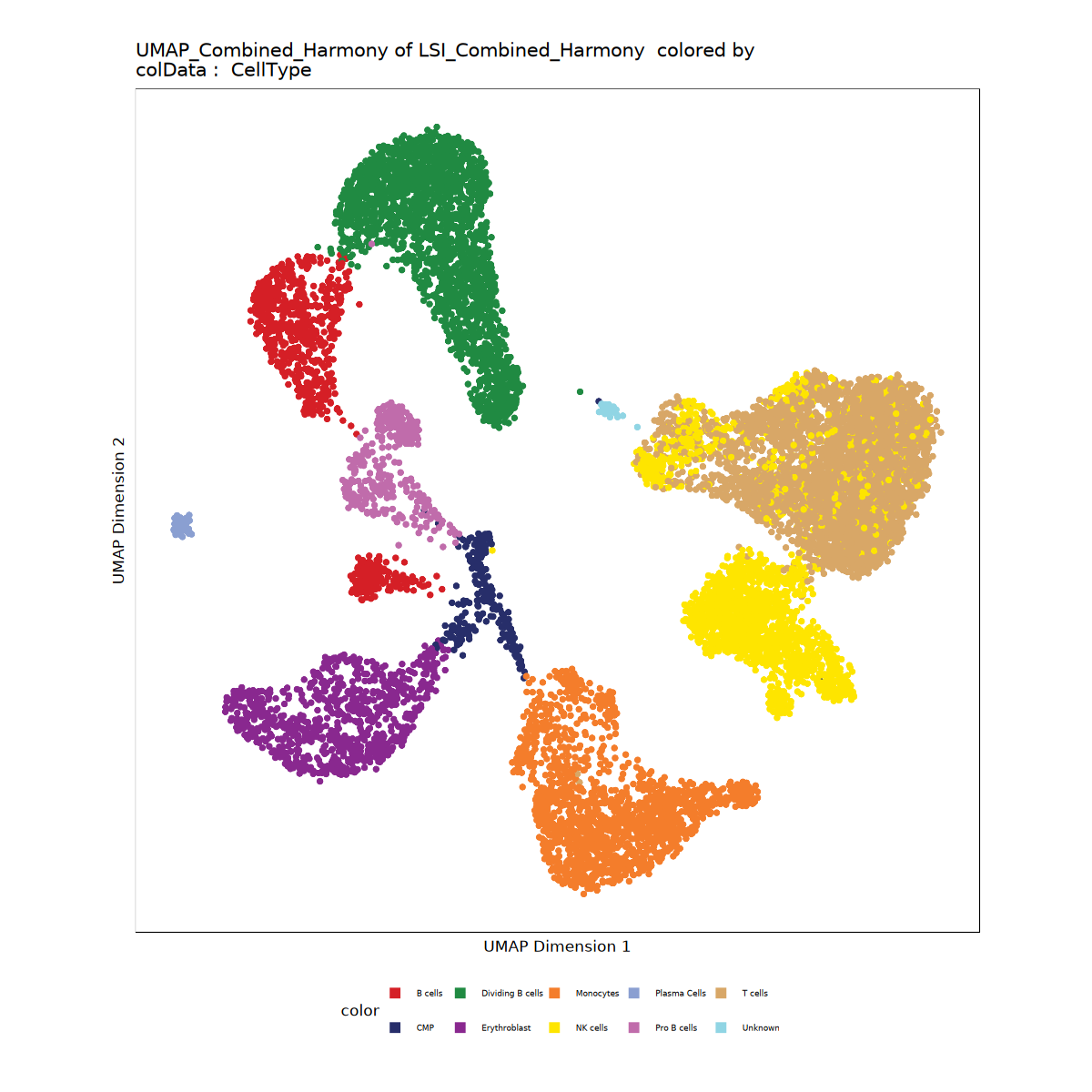

9. Saving Results

projMulti_filtered <- saveArchRProject(ArchRProj = projMulti_filtered, outputDirectory = "Save-ProjMulti2", overwrite = TRUE, load = TRUE)