ATAC + RNA Multi-omics: DORC Analysis

Author: SeekGene

Time: 26 min

Words: 5.1k words

Updated: 2026-07-07

Reads: 0 times

1. Tutorial Overview

This tutorial leverages single-cell multi-omics analysis tools including Seurat and Signac, and is dedicated to in-depth DORC (Domains of Regulatory Chromatin) analysis on SeekArc single-cell multi-omics data (scRNA-seq + scATAC-seq). This tutorial is intended for SeekArc multi-omics data that have already undergone basic quality control, cell-population annotation, and preliminary Peak Calling. By integrating chromatin accessibility with gene expression levels, it achieves the following three core analytical objectives:

• Peak–Gene Association Network Construction (Peak-to-Gene Linkage): Based on the co-variation hypothesis, compute the correlation between each gene and each Peak in its vicinity (typically within a range of several hundred kb), identifying Peak–Gene regulatory pairs with significant cis-regulatory relationships.
• DORC Gene Identification: Breaking through the limitation of single-enhancer regulation, search for "super target genes" coordinately controlled by a large number (e.g., ≥ 10) of cis-regulatory elements. These DORC genes are typically core regulatory hubs that determine cell fate, maintain cell state, or drive disease progression.
• DORC Activity Assessment and Cell-Specificity Analysis (Activity Scoring & Differential Analysis): Integrate the accessibility signals of multiple Peaks associated with each DORC gene to quantify their comprehensive regulatory activity at single-cell resolution, and reveal the deep biological mechanisms determining specific cellular states through differential analysis and clustering heatmaps.

suppressPackageStartupMessages(suppressWarnings({
    library(future)
    library(Seurat)
    library(BiocGenerics)
    library(S4Vectors)
    library(IRanges)
    library(Signac)
    library(ComplexHeatmap)
    library(Biobase)
    library(AnnotationDbi)
    library(stringr)
    library(dplyr)
    library(foreach)
    library(doParallel)
}))

2. Input Files and Parameter Configuration

2.1 Input File Requirements

This analysis tutorial performs DORC (Domains of Regulatory Chromatin) analysis based on a pre-processed Seurat multi-omics object. Before starting, the following core input files need to be prepared:

• input.rds: The pre-processed Seurat object file. This object must contain both RNA and ATAC assays, and the ATAC modality must have already undergone basic Peak Calling as well as dimensionality reduction and clustering analysis.
• meta.tsv: Cell metadata file (tab-separated, optional). Used to provide additional cell annotation information. Must contain columns defining cell type and sample grouping, enabling subsequent precise extraction of cell subpopulations and dimensionality reduction/clustering analyses as needed.
• genome.fa: Reference genome FASTA file for the corresponding species. Its main purpose is to extract the actual DNA sequences based on the genomic coordinates of ATAC peaks, providing underlying sequence support for subsequent computation of Peak sequence features such as GC content and length (RegionStats), thereby constructing the background null model for Peak–Gene correlation.

2.2 Core Parameter Configuration

The following parameters control file paths, filtering thresholds, and analysis details. Please modify them according to your actual data:

# rds: Path to the input Seurat object RDS file; must contain pre-processed RNA and ATAC data.
rds = "/path/to/input.rds"

# meta: Path to the cell metadata file (TSV format), used to provide additional grouping or sample information. Leave empty if not needed.
meta = "/path/to/meta.tsv"

# genome_file: Path to the reference genome FASTA file for the corresponding species, used to extract sequences for Motif analysis.
genome_file = "/path/to/genome.fa"

# dorc_peak_thresh: Threshold for defining DORC genes (typically set at ≥ 10 associated Peaks).
dorc_peak_thresh = "10"

# clusters_col: Specifies which column in the metadata serves as the grouping basis for cell subpopulations (e.g., cell type).
clusters_col = "Celltype"

# celltypes: Comma-separated string specifying the names of cell subpopulations to include in the analysis.
celltypes = "B cells,CMP,Dividing B cells,Erythroblast,NK cells,pDC,Plasma Cells,Pro B cells,T cells"

# sample_col: Specifies which column in the metadata serves as the sample batch discriminator.
sample_col = "Sample"

# samples: Comma-separated string specifying the names of samples to include in the analysis.
samples = "25030508_pbmc_1_arc,XYRD_pbmc_2_arc"

# filter: Logical value string ("TRUE"/"FALSE"), whether to perform significance and variance filtering on Peak–Gene association pairs before analysis.
filter = "FALSE"

# corCutOff: Correlation score filtering threshold (absolute value). Only effective when filter is TRUE.
corCutOff = ""

# pCutOff: P-value significance filtering threshold. Only effective when filter is TRUE.
pCutOff = ""

# downsample: Logical value string ("True"/"False"), whether to randomly downsample each cell subpopulation before analysis to save memory.
downsample = "True"

# downsample_num: Downsample count — the maximum number of cells retained per cell subpopulation. Only effective when downsample is "True".
downsample_num = "500"

dorc_peak_thresh <- as.numeric(dorc_peak_thresh)

outdir <- "./result/"
dir.create(outdir, recursive = TRUE)

celltypes <- strsplit(celltypes,",")[[1]]
samples <- strsplit(samples,",")[[1]]

filter <- as.logical(filter)
corCutOff <- as.numeric(corCutOff)
pCutOff <- as.numeric(pCutOff)

3. Data Loading and Preprocessing

3.1 Environment Initialization and Parallel Computing

Before formally loading the data, set the number of parallel cores and memory limits to accelerate subsequent analysis steps.

if (requireNamespace("future", quietly = TRUE)) {
    cores <- parallelly::availableCores()
    workers <- as.integer(floor(cores * 0.7))
    
    if (.Platform$OS.type == "unix") {
        future::plan(future::multicore, workers = workers)
    } else {
        future::plan(future::multisession, workers = workers)
    }
    
    message("total cores =", cores, "，uses ", workers, " works")
}

if (requireNamespace("memuse", quietly = TRUE)) {
    total_mem <- memuse::Sys.meminfo()$totalram
    total_mem_bytes <- as.numeric(total_mem)
    future_mem <- total_mem_bytes * 0.7
    future_mem_gb <- future_mem / 1024^3
    total_mem_gb <- total_mem_bytes / 1024^3
} else {
    future_mem <- 50 * 1024^3
    future_mem_gb <- 50
    total_mem_gb <- 50 / 0.6
}
options(future.globals.maxSize = future_mem)

3.2 Loading the Seurat Object and Metadata

Read the pre-processed multi-omics object and integrate additional cell classification information as needed.

obj <- readRDS(rds)
if (meta != ""){
  meta <- read.table(meta,header=T,sep='\t',check.names=F)
  #rownames(meta) <- meta$barcodes
  rownames(meta) <- meta$barcode
  obj <- AddMetaData(obj, meta)
}
Idents(obj) <- obj@meta.data[[clusters_col]]

3.3 Cell Type Selection and Downsample Balancing

To reduce false-positive correlations caused by the extremely large quantity of certain cell types, and to control overall memory consumption during analysis, specific cell populations can be extracted based on the celltypes parameter, and the downsample mechanism can be enabled to randomly sample overly large cell populations.

if (exists("downsample") && downsample != "" && !is.na(as.logical(downsample)) && as.logical(downsample)) {
  if (exists("downsample_num") && downsample_num != "" && !is.na(as.numeric(downsample_num)) && as.numeric(downsample_num) > 1) {
    obj <- subset(obj, downsample = as.numeric(downsample_num))
  }
}

obj <- subset(obj, subset = !!sym(clusters_col) %in% celltypes)
obj <- subset(obj, subset = !!sym(sample_col) %in% samples)

v <- obj@meta.data[[clusters_col]]
sorted_levels <- str_sort(unique(as.character(v)), numeric = TRUE, na_last = TRUE)
obj@meta.data[[clusters_col]] <- factor(v, levels = sorted_levels, ordered = TRUE)

3.4 Reference Genome Processing

To prepare for sequence feature extraction (RegionStats) in downstream Peak-to-Gene association analysis, the genome sequence file must first be processed: read genome.fa and convert it into a DNAStringSet object, while aligning the chromosome names of ATAC peaks in the object (retaining only shared chromosome information).

DefaultAssay(obj) <- "ATAC"
Idents(obj) <- clusters_col

library(Biostrings)
genome <- readDNAStringSet(genome_file)
names(genome) <- sub(" .*", "", names(genome)) 
keep_chromosomes <- unique(as.character(seqnames(granges(obj[["ATAC"]]))))
genome <- genome[which(names(genome) %in% keep_chromosomes)]
obj@assays$ATAC@ranges <- keepSeqlevels(granges(obj),keep_chromosomes, pruning.mode="coarse")

4. Peak-to-Gene Association Analysis Across Cell Populations

Peak-to-Gene (LinkPeaks) association analysis is the core prerequisite step for DORC identification.

• Why must LinkPeaks be performed before DORC analysis?

The essence of DORC (Domains of Regulatory Chromatin) is "genes under the dense, cooperative control of cis-regulatory elements." Therefore, to identify these super regulatory hubs, we must first exhaustively enumerate and verify, across the genome, whether a genuine regulatory relationship exists between every Peak and every potential target gene.

The traditional linear distance hypothesis (e.g., simply assuming that the Peak closest to the TSS is the enhancer regulating that gene) has severe limitations, because three-dimensional chromatin folding allows distal enhancers to regulate target genes across hundreds of kb. Therefore, this step adopts a "co-variation-driven" strategy: using the LinkPeaks algorithm provided by Signac, compute the statistical correlation between each Peak's accessibility and the expression level of nearby genes at the cross-cell (Pseudobulk) level.

• Core Logic: If changes in a Peak's accessibility are consistently accompanied by synchronous fluctuations in a specific target gene's expression, we consider that Peak to be a genuine enhancer driving that gene's transcription. Only after this most basic "one-to-one" regulatory connection network is constructed can we proceed in subsequent steps to count "which genes are associated with an abnormally large number (≥ 10) of regulatory elements," thereby completing the final DORC gene identification.

invisible(capture.output({
  suppressMessages(suppressWarnings({ 
    links_all <- Signac::Links(obj[["ATAC"]]) 
    
    if (length(links_all) == 0) { 
    
      obj <- RegionStats( 
        object = obj, 
        genome = genome, 
        assay = "ATAC" 
      ) 
      
      obj <- LinkPeaks( 
          object = obj, 
          peak.assay = "ATAC", 
          expression.assay = "RNA" 
      ) 
      
      links_all <- Signac::Links(obj[["ATAC"]]) 
      
      if (length(links_all) == 0) { 
        stop("未找到peak-to-gene链接") 
      } 
    } 
    
    write.table( 
      as.data.frame(links_all), 
      file = file.path(outdir, "Gene2PeakLinks.xls"), 
      sep = "\t", 
      row.names = FALSE, 
      col.names = TRUE, 
      quote = FALSE 
    )          
  }))
}))

saveRDS(obj, file.path(outdir, "output.rds"))

5. DORC Gene Identification and Analysis

This is the most core analytical step in this tutorial. Building on the global Peak-to-Gene association analysis, we will further introduce the concept of DORC (Domains of Regulatory Chromatin) to scan the genome for super regulatory hubs, enabling DORC identification and downstream analyses and visualization.

dorc_use_filter <- filter

links_dorc <- as.data.frame(links_all)
links_dorc <- links_dorc[, c("peak", "gene", "score", "pvalue")]

5.1 DORC Gene Identification

Systematically inventory all significant Peak–Gene connections, counting the total number of cis-regulatory elements (Peaks) associated with each target gene across the genome. Set a stringent background threshold (controlled by the dorc_peak_thresh parameter, typically set at ≥ 10 associated Peaks). When the number of regulatory elements associated with a specific gene significantly exceeds this threshold, that gene is defined as a DORC gene.

plotGeneLinkCountRank <- function(links, dorc_peak_thresh = 10, label_n = 10, seed = 1) {
  set.seed(seed)
  link_df <- data.frame(
    gene = links$gene,
    peak = links$peak,
    stringsAsFactors = FALSE
  )
  link_df <- link_df[!is.na(link_df$gene) & !is.na(link_df$peak), , drop = FALSE]
  
  gene_link_df <- link_df %>%
    dplyr::distinct(gene, peak) %>%
    dplyr::count(gene, name = "link_count") %>%
    dplyr::arrange(link_count) %>%
    dplyr::mutate(
      rank = dplyr::row_number(),
      is_dorc = link_count > dorc_peak_thresh
    )
    
  n_dorc <- sum(gene_link_df$is_dorc)

  total_genes <- nrow(gene_link_df)
  split_x <- total_genes - n_dorc + 0.5
  ymax <- max(gene_link_df$link_count, na.rm = TRUE)

  dorc_genes_df <- gene_link_df %>% dplyr::filter(is_dorc == TRUE)
  label_data <- data.frame()
  if (nrow(dorc_genes_df) > 0) {
    n_sample <- min(label_n, nrow(dorc_genes_df))
    label_data <- dorc_genes_df %>%
      dplyr::arrange(dplyr::desc(link_count)) %>%
      dplyr::slice_head(n = n_sample)
  }
  
  dorc_color <- "#4A90E2"
  
label_x <- total_genes / 2

p <- ggplot2::ggplot(gene_link_df, ggplot2::aes(x = rank, y = link_count)) +
  ggplot2::geom_line(linewidth = 1) +
  ggplot2::geom_point(ggplot2::aes(color = is_dorc), size = 1.2, alpha = 0.9) +
  ggplot2::geom_vline(xintercept = split_x, linetype = "dashed", color = dorc_color) +
  ggplot2::geom_hline(yintercept = dorc_peak_thresh, linetype = "dashed", color = "grey50") +
  ggplot2::scale_color_manual(values = c("TRUE" = dorc_color, "FALSE" = "grey70"), guide = "none") +
  ggplot2::annotate(
    "text",
    x = label_x,
    y = ymax,
    label = paste0("DORC n=", n_dorc),
    vjust = -0.6,
    hjust = 0.5,
    color = dorc_color,
    size = 4
  ) +
  ggplot2::labs(
    x = "Rank of genes by linked peak count (Ascending)",
    y = "Number of linked peaks per gene"
  ) +
  ggplot2::theme_classic() +
  ggplot2::theme(
    legend.position = "none",
  # text = element_text(family = "sans"),
    axis.title = ggplot2::element_text(size = 14),
    axis.text = ggplot2::element_text(size = 12),
    plot.title = ggplot2::element_text(hjust = 0.5, size = 14),
    axis.text.x = ggplot2::element_blank(),
    axis.ticks.x = ggplot2::element_blank()
  )
    
  if (nrow(label_data) > 0) {
    p <- p + ggrepel::geom_text_repel(
      data = label_data,
      ggplot2::aes(label = gene),
      color = "black",
      size = 3,
      box.padding = 0.5,
      point.padding = 0.3,
      force = 0.03,
      max.overlaps = 50,
      segment.color = "grey50",
      nudge_x = -0.1 * total_genes,
      direction = "y"
    )
  }
  
  return(p)
}

options(repr.plot.width = 10, repr.plot.height = 5)
print(plotGeneLinkCountRank(links_all, dorc_peak_thresh = dorc_peak_thresh))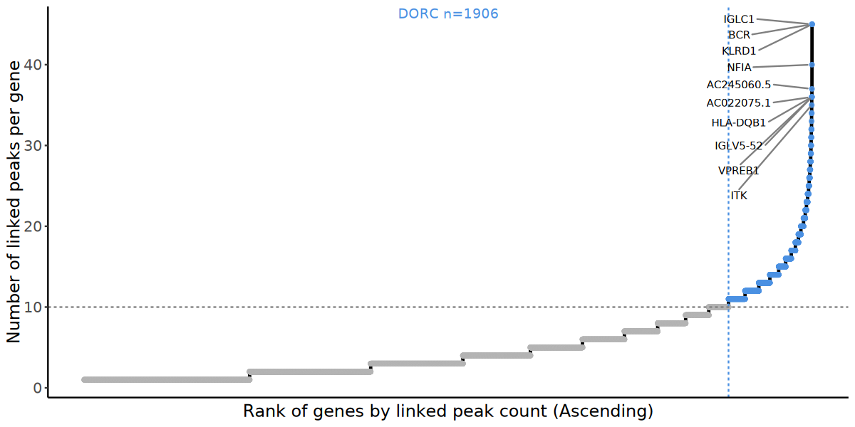

💡 Plot InterpretationDORC Gene Identification Ranking Plot (Peak2GeneGeneLinkCountRank):

• X-axis: Represents all target genes. Genes are arranged in ascending order by the number of associated Peaks (from fewest to most).
• Y-axis: Represents the absolute number of Peaks significantly associated with each target gene across the genome.
• Dashed Line Meaning: The horizontal gray dashed line represents the cutoff threshold defining DORC genes (by default, ≥ 10 associated Peaks); the vertical blue dashed line separates the super-regulatory genes on the right satisfying the threshold condition (blue dots) from the ordinary genes on the left (gray dots).
• Text Annotation: The top of the plot annotates the total number of identified DORC genes, while on the right dense region a subset of representative DORC gene names is randomly sampled and bold-marked to help researchers quickly pinpoint potential key core driver genes.

5.2 DORC Activity Assessment

Compute the cumulative accessibility of all Peaks targeting the same DORC gene in each cell, generating a single-cell-level DORC activity score (Accessibility Score) matrix. This is not merely a simple counting process. We weight or aggregate the ATAC accessibility signals (Pseudobulk Counts) of all associated Peaks belonging to the same DORC gene, thereby producing a comprehensive "DORC Score" for each cell population that represents the overall upstream regulatory strength of that DORC gene.

invisible(capture.output({
  suppressMessages(suppressWarnings({
    
    links_dorc <- links_dorc[!is.na(links_dorc$peak) & !is.na(links_dorc$gene), , drop = FALSE] 
    
    if (dorc_use_filter) { 
      links_dorc <- links_dorc[abs(links_dorc$score) >= corCutOff & links_dorc$pvalue <= pCutOff, , drop = FALSE] 
    } 
    
    if (nrow(links_dorc) == 0) { 
      stop("DORC analysis failed") 
    } 
    
    atac_counts <- GetAssayData(obj, assay = "ATAC", slot = "counts") 
    if (!inherits(atac_counts, "dgCMatrix")) atac_counts <- as(atac_counts, "dgCMatrix") 
    
    peak_idx <- match(links_dorc$peak, rownames(atac_counts)) 
    if (any(is.na(peak_idx))) { 
      stop("DORC analysis failed.") 
    } 
    
    peak_idx_by_gene <- split(peak_idx, links_dorc$gene) 
    peak_idx_by_gene <- lapply(peak_idx_by_gene, unique) 
    peak_count <- vapply(peak_idx_by_gene, length, integer(1)) 
    peak_idx_by_gene <- peak_idx_by_gene[peak_count > dorc_peak_thresh] 
    
    if (length(peak_idx_by_gene) == 0) { 
      stop(paste0("DORC analysis failed.", dorc_peak_thresh)) 
    } 
    
    peak_count <- vapply(peak_idx_by_gene, length, integer(1)) 
    gene_names <- names(peak_idx_by_gene) 
    
    cell_sums <- Matrix::colSums(atac_counts) 
    cell_sums[cell_sums == 0] <- 1 
    scale_diag <- Matrix::Diagonal(x = 1e6 / cell_sums) 
    atac_cpm <- atac_counts %*% scale_diag 
    
    dorc_mat <- matrix(0, nrow = ncol(atac_cpm), ncol = length(gene_names)) 
    rownames(dorc_mat) <- colnames(atac_counts) 
    colnames(dorc_mat) <- gene_names 
    
    for (i in seq_along(gene_names)) { 
      idx <- peak_idx_by_gene[[i]] 
      if (length(idx) == 1) { 
        dorc_mat[, i] <- as.numeric(atac_cpm[idx, ]) 
      } else { 
        dorc_mat[, i] <- as.numeric(Matrix::colSums(atac_cpm[idx, , drop = FALSE])) 
      } 
    } 
    
    peak_sum_df <- data.frame( 
      peak_count = peak_count, 
      row.names = gene_names 
    ) 
    peak_sum_sorted <- peak_sum_df[order(peak_sum_df$peak_count, decreasing = TRUE), , drop = FALSE] 
    
    output_dorc_peaks <- file.path(outdir, paste0("DORC_peaks_thresh", dorc_peak_thresh, "_sum_sorted.tsv")) 
    write.table(peak_sum_sorted, output_dorc_peaks, sep = "\t", row.names = TRUE, col.names = FALSE, quote = FALSE) 
    
    output_dorc <- file.path(outdir, paste0("DORC_scores_thresh", dorc_peak_thresh, ".tsv")) 
    write.table(dorc_mat, output_dorc, sep = "\t", row.names = TRUE, col.names = NA, quote = FALSE) 
    
    saveRDS(dorc_mat, file.path(outdir, paste0("DORC_scores_thresh", dorc_peak_thresh, ".rds"))) 
    
  }))
}))

5.3 DORC Activity Differential Analysis

Based on the single-cell DORC activity score matrix constructed in the previous step, perform differential activity analysis using Seurat's FindAllMarkers function. This step aims to identify DORC genes that specifically exhibit high regulatory activity in each cell subpopulation, thereby pinpointing the landmark regulatory hubs that maintain specific population homeostasis or drive their differentiation.

invisible(capture.output({
  suppressMessages(suppressWarnings({
    
    dorc_df <- as.data.frame(dorc_mat, check.names = FALSE) 
    if (!all(colnames(obj) %in% rownames(dorc_df))) { 
      stop("DORC analysis failed.") 
    } 
    dorc_df <- dorc_df[colnames(obj), , drop = FALSE] 
    
    dorc_meta <- dorc_df 
    colnames(dorc_meta) <- paste0(colnames(dorc_meta), "_dorc") 
    existing_dorc_meta <- intersect(colnames(obj@meta.data), colnames(dorc_meta)) 
    if (length(existing_dorc_meta) > 0) { 
      obj@meta.data <- obj@meta.data[, setdiff(colnames(obj@meta.data), existing_dorc_meta), drop = FALSE] 
    } 
    obj@meta.data <- cbind(obj@meta.data, dorc_meta[rownames(obj@meta.data), , drop = FALSE]) 
    
    dorc_assay_mat <- t(as.matrix(dorc_df)) 
    if (!inherits(dorc_assay_mat, "dgCMatrix")) { 
      dorc_assay_mat <- as(dorc_assay_mat, "dgCMatrix") 
    } 
    obj[["DORC"]] <- CreateAssayObject(counts = dorc_assay_mat) 
    
    if (!(clusters_col %in% colnames(obj@meta.data))) { 
      stop("DORC analysis failed.", clusters_col) 
    } 
    Idents(obj) <- as.factor(as.character(obj@meta.data[[clusters_col]])) 
    DefaultAssay(obj) <- "DORC" 
    
    markers_dorc <- FindAllMarkers( 
      object = obj, 
      assay = "DORC", 
      only.pos = TRUE, 
      logfc.threshold = 0, 
      min.pct = 0.05 
    ) 
    
    if (!"gene" %in% colnames(markers_dorc)) { 
      markers_dorc$gene <- rownames(markers_dorc) 
    } 
    output_dorc_markers <- file.path(outdir, "DORC_FindAllMarkers.tsv") 
    write.table(markers_dorc, output_dorc_markers, sep = "\t", row.names = FALSE, col.names = TRUE, quote = FALSE)     
    markers_sig <- markers_dorc[!is.na(markers_dorc$p_val_adj) & markers_dorc$p_val_adj < 0.05 & markers_dorc$avg_log2FC > 0, , drop = FALSE] 
    if (nrow(markers_sig) == 0) { 
      stop("DORC analysis failed.") 
    } 
    
    markers_top10 <- markers_sig %>% 
      group_by(cluster) %>% 
      slice_max(n = 10, order_by = avg_log2FC, with_ties = FALSE) %>% 
      ungroup() 
    
    output_top10 <- file.path(outdir, "DORC_top10_per_cluster_markers.tsv") 
    write.table(markers_top10, output_top10, sep = "\t", row.names = FALSE, col.names = TRUE, quote = FALSE) 

  }))
}))

head(markers_sig)

A data.frame: 6 × 7

	p_val	avg_log2FC	pct.1	pct.2	p_val_adj	cluster	gene
	<dbl>	<dbl>	<dbl>	<dbl>	<dbl>	<fct>	<chr>
DTX1	2.397218e-189	2.463573	0.924	0.462	4.569098e-186	B cells	DTX1
RASAL1	1.771071e-171	2.109955	0.942	0.588	3.375661e-168	B cells	RASAL1
CFAP73	2.060654e-165	2.016315	0.944	0.598	3.927607e-162	B cells	CFAP73
IGLC1	2.272933e-163	1.590690	0.994	0.796	4.332209e-160	B cells	IGLC1
TCL6	8.499601e-160	1.902479	0.944	0.530	1.620024e-156	B cells	TCL6
SLC8B1	5.623266e-158	1.932736	0.942	0.637	1.071795e-154	B cells	SLC8B1

💡 Interpretation Guide: DORC (Domains of Regulatory Chromatin) Differential Analysis Result Table

This table displays the DORC genes identified via Seurat FindAllMarkers as having population-specific high regulatory activity across cell subpopulations. The DORC score reflects the cumulative composite effect of signals from multiple open chromatin regions near the gene and serves as an important hallmark of strong enhancer-regulated genes. It is recommended to prioritize by combining p_val_adj and avg_log2FC.

• gene: Name of the DORC gene — i.e., those target genes strongly driven by multiple cis-regulatory elements.
• cluster: Name or number of the target cell subpopulation in which this DORC gene exhibits significantly high regulatory activity.
• p_val: Raw significance P-value of the differential analysis.
• avg_log2FC: Average Log2 fold change. A positive value indicates that the comprehensive regulatory activity of this DORC gene in the current cluster is higher than in other cell populations. The larger the value, the stronger the population-specific regulatory intensity.
• pct.1: Detection (activation) proportion of this gene as a DORC in the current cluster, ranging from 0 to 1.
• pct.2: Detection (activation) proportion of this gene as a DORC across all other cell subpopulations as background, ranging from 0 to 1.
• p_val_adj: P-value after multiple-testing correction — the gold standard for determining whether this gene is a significant DORC marker of the subpopulation.

5.4 DORC Activity UMAP Spatial Visualization

Based on the Top 10 subpopulation-specific DORC genes extracted from each cell subpopulation, intuitively present their single-cell-level activity distribution in UMAP dimensionality-reduction space via FeaturePlot. Since DORC score differences can be extremely large, a log10 transformation and quantile truncation are performed in advance to smooth extreme values.

DefaultAssay(obj) <- "DORC"

features_to_show <- markers_top10$gene
features_to_show <- unique(features_to_show)
features_to_show <- features_to_show[features_to_show %in% rownames(obj[["DORC"]])]

plot_output_dir <- file.path(outdir, "DORC_FeaturePlot_5in1")
dir.create(plot_output_dir, recursive = TRUE, showWarnings = FALSE)

plot_dorc_feature <- function(gene, obj) {
  values <- as.numeric(GetAssayData(obj, assay = "DORC", slot = "data")[gene, ])
  values <- values[is.finite(values)]
  if (length(values) == 0) return(NULL)

  scaled_values <- log10(values + 1)
  
  plot_col_name <- paste0("Log10_", gsub("-", "_", gene))
  obj@meta.data[[plot_col_name]] <- scaled_values

  p1 <- as.numeric(quantile(scaled_values, 0.01, na.rm = TRUE))
  p99 <- as.numeric(quantile(scaled_values, 0.99, na.rm = TRUE))

  custom_colors <- c("#313695", "#4575b4", "#74add1", "#abd9e9", "#e0f3f8", 
                     "#ffffbf", "#fee090", "#fdae61", "#f46d43", "#d73027", "#a50026")

  FeaturePlot(
    object = obj,
    features = plot_col_name,
    reduction = "umap",
    min.cutoff = p1,
    max.cutoff = p99,
    pt.size = 0.3
  ) +
    ggplot2::scale_color_gradientn(
      colors = custom_colors,
      name = "log10(DORC+1)"
    ) +
    ggplot2::ggtitle(gene) +
    ggplot2::theme(plot.title = ggplot2::element_text(size = 10, hjust = 0.5))
}

save_and_encode_plot <- function(plot, filename_base, width = 26, height = 3.8) {
  full_path_pdf <- paste0(filename_base, ".pdf")
  full_path_png <- paste0(filename_base, ".png")

  ggplot2::ggsave(full_path_pdf, plot, width = width, height = height)
  ggplot2::ggsave(full_path_png, plot, width = width, height = height, dpi = 100)


  if (file.exists(full_path_png)) {
    return(list(png_path = full_path_png, pdf_path = full_path_pdf))
  }
  NULL
}

suppressMessages(suppressWarnings({
feature_groups <- split(
  features_to_show,
  ceiling(seq_along(features_to_show) / 5)
)

plot_list <- list()

for (i in seq_along(feature_groups)) {
  genes <- feature_groups[[i]]

  p_list <- lapply(genes, function(g) plot_dorc_feature(g, obj))
  p_list <- p_list[!vapply(p_list, is.null, logical(1))]
  if (length(p_list) == 0) next

  if (length(p_list) < 5) {
    p_list <- c(p_list, replicate(5 - length(p_list), patchwork::plot_spacer(), simplify = FALSE))
  }

  combined_plot <- patchwork::wrap_plots(p_list, ncol = 5) +
    patchwork::plot_annotation(title = paste0("DORC FeaturePlot Group ", i))

  file_base <- file.path(plot_output_dir, paste0("DORC_group_", sprintf("%03d", i)))
  res <- save_and_encode_plot(combined_plot, file_base, width = 26, height = 3.8)
}

}))

options(repr.plot.width = 23, repr.plot.height = 4)
combined_plot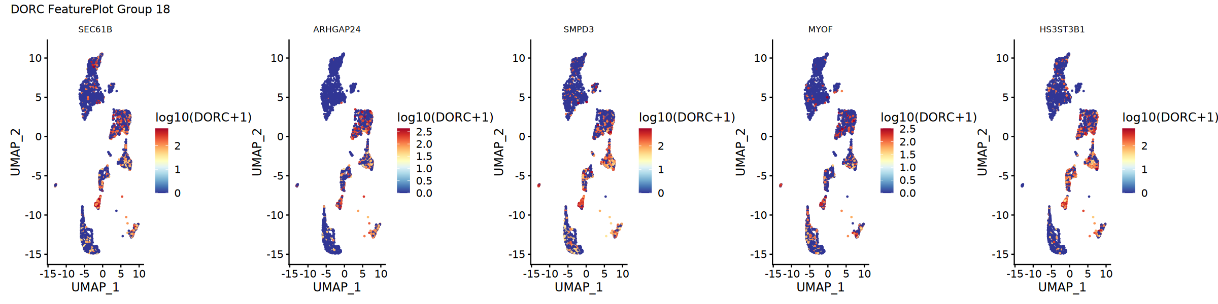

💡 Interpretation Guide: Differential DORC Gene UMAP Feature Mapping Plot (FeaturePlot)

This example plot displays the spatial distribution and relative regulatory activity of each core driver gene (DORC gene) across different single-cell populations. All other differential DORC results are located in the .result/DORC_FeaturePlot_5in1 directory.

• Scatter Points (Cells): Each scatter point in the plot represents a single cell; its relative position in two-dimensional space reflects the overall transcriptomic or chromatin-state similarity between cell populations.
• Color Gradient (Activity Score): The color reflects the log-smoothed value of the cumulative accessibility score of a specific DORC gene in that cell (log10(DORC+1)).
  • Dark blue: Represents inactive or extremely low activity.
  • Yellow-green: Represents a moderate transitional state.
  • Orange to dark red: Indicates that the multiple enhancer elements associated with this gene are highly open in that cell, with extremely strong regulatory activity.
• Numerical Smoothing and Truncation: Since raw DORC peak counts often contain extreme high values, a Log10 log transformation is pre-applied to smooth extreme differences; simultaneously, the upper and lower bounds of the color mapping are truncated using the 1st and 99th percentiles of the smoothed data to ensure that subtle biological variation patterns are clearly visible.
• Group Display: The data table at the bottom of the figure is paginated in a format of 5 genes per group. Clicking the thumbnail opens the high-resolution PDF vector plot in a new tab.

5.5 DORC Population-Level Activity Heatmap (Pseudobulk Heatmap)

To present the core DORC gene activity patterns across cell subpopulations from a global perspective, we aggregate the single-cell-level DORC matrix by cell subpopulation (Pseudobulk) and compute average activity. Then we extract the Top 10 specific DORC genes for each subpopulation, apply Z-score normalization, and plot a hierarchical clustering heatmap.

# ---- Code cell 61 ----
markers_top10_by_cluster <- markers_sig %>%
  group_by(cluster) %>%
  arrange(desc(avg_log2FC), .by_group = TRUE) %>%
  slice_head(n = 10) %>%
  ungroup()

output_top10_by_cluster <- file.path(outdir, "DORC_top10_by_cluster.tsv")
write.table(markers_top10_by_cluster, output_top10_by_cluster, sep = "\t", row.names = FALSE, col.names = TRUE, quote = FALSE)

selected_dorc_genes <- unique(markers_top10_by_cluster$gene)
selected_dorc_genes <- selected_dorc_genes[selected_dorc_genes %in% rownames(obj[["DORC"]])]
if (length(selected_dorc_genes) == 0) {
  stop("DORC analysis failed.")
}

dorc_selected_cells_by_gene <- t(as.matrix(GetAssayData(obj, assay = "DORC", slot = "data")[selected_dorc_genes, , drop = FALSE]))
cell_groups <- as.character(obj@meta.data[[clusters_col]])
names(cell_groups) <- rownames(obj@meta.data)
cell_groups <- cell_groups[rownames(dorc_selected_cells_by_gene)]
valid_cells <- !is.na(cell_groups) & cell_groups != ""
dorc_selected_cells_by_gene <- dorc_selected_cells_by_gene[valid_cells, , drop = FALSE]
cell_groups <- cell_groups[valid_cells]

dorc_pb_sum <- rowsum(dorc_selected_cells_by_gene, group = cell_groups, reorder = FALSE)
dorc_pb_n <- as.numeric(table(cell_groups)[rownames(dorc_pb_sum)])
dorc_pb_mean <- dorc_pb_sum / dorc_pb_n
dorc_pb_gene_by_celltype <- t(dorc_pb_mean)

output_pb <- file.path(outdir, "DORC_pseudobulk_top10ByCluster.tsv")
write.table(dorc_pb_gene_by_celltype, output_pb, sep = "\t", row.names = TRUE, col.names = NA, quote = FALSE)

dorc_pb_scaled <- t(scale(t(dorc_pb_gene_by_celltype)))
dorc_pb_scaled[is.na(dorc_pb_scaled)] <- 0


n_celltypes <- ncol(dorc_pb_scaled)
labels_per_cluster <- if (n_celltypes <= 5) {
  5L
} else if (n_celltypes < 8) {
  4L
} else if (n_celltypes <= 10) {
  3L
} else if (n_celltypes <= 15) {
  2L
} else {
  1L
}

markers_ranked_by_cluster <- markers_top10_by_cluster %>%
  group_by(cluster) %>%
  arrange(desc(avg_log2FC), .by_group = TRUE) %>%
  ungroup() %>%
  filter(gene %in% rownames(dorc_pb_scaled))

clusters <- unique(as.character(markers_ranked_by_cluster$cluster))
used_genes <- character()
anno_labels <- character()
for (cl in clusters) {
  genes <- as.character(markers_ranked_by_cluster$gene[markers_ranked_by_cluster$cluster == cl])
  genes <- genes[!is.na(genes) & genes != ""]
  genes <- genes[genes %in% rownames(dorc_pb_scaled)]
  preferred <- genes[!genes %in% used_genes]
  picked <- head(preferred, labels_per_cluster)
  if (length(picked) < labels_per_cluster) {
    picked <- c(picked, head(setdiff(genes, picked), labels_per_cluster - length(picked)))
  }
  used_genes <- c(used_genes, picked)
  anno_labels <- c(anno_labels, picked)
}

row_hc <- stats::hclust(stats::dist(dorc_pb_scaled))
anno_df <- data.frame(
  label = anno_labels,
  row_index = match(anno_labels, rownames(dorc_pb_scaled)),
  stringsAsFactors = FALSE
)
anno_df <- anno_df[!is.na(anno_df$row_index), , drop = FALSE]
anno_df <- anno_df[!duplicated(anno_df$row_index), , drop = FALSE]
anno_at <- anno_df$row_index
anno_labels <- anno_df$label

row_anno <- NULL
anno_width_cm <- 0
if (length(anno_at) > 0) {
  anno_width_cm <- max(4.5, min(8, max(nchar(anno_labels)) * 0.25))
  row_anno <- ComplexHeatmap::rowAnnotation(
    mark = ComplexHeatmap::anno_mark(
      at = anno_at,
      labels = anno_labels,
      which = "row",
      side = "right",
      labels_gp = grid::gpar(fontsize = 12),
      lines_gp = grid::gpar(col = "grey50", lwd = 0.8)
    ),
    width = grid::unit(anno_width_cm, "cm")
  )
}

output_pb_pdf <- file.path(outdir, "DORC_pseudobulk_top10ByCluster_heatmap.pdf")
pdf(output_pb_pdf, width = 12, height = 9)
ht <- ComplexHeatmap::Heatmap(
  dorc_pb_scaled,
  name = "DORC Z-score",
  col = circlize::colorRamp2(c(-2, 0, 2), c("#2166AC", "white", "#B2182B")),
  cluster_rows = row_hc,
  cluster_columns = TRUE,
  show_row_names = FALSE,
  show_row_dend = FALSE,
  show_column_dend = FALSE,
  show_column_names = TRUE,
  right_annotation = row_anno,
  column_names_gp = grid::gpar(fontsize = 12)
)
draw(ht)
invisible(dev.off())

saveRDS(obj, file.path(outdir, "output_with_dorc_downstream.rds"))

options(repr.plot.width = 15, repr.plot.height = 8)
draw(ht)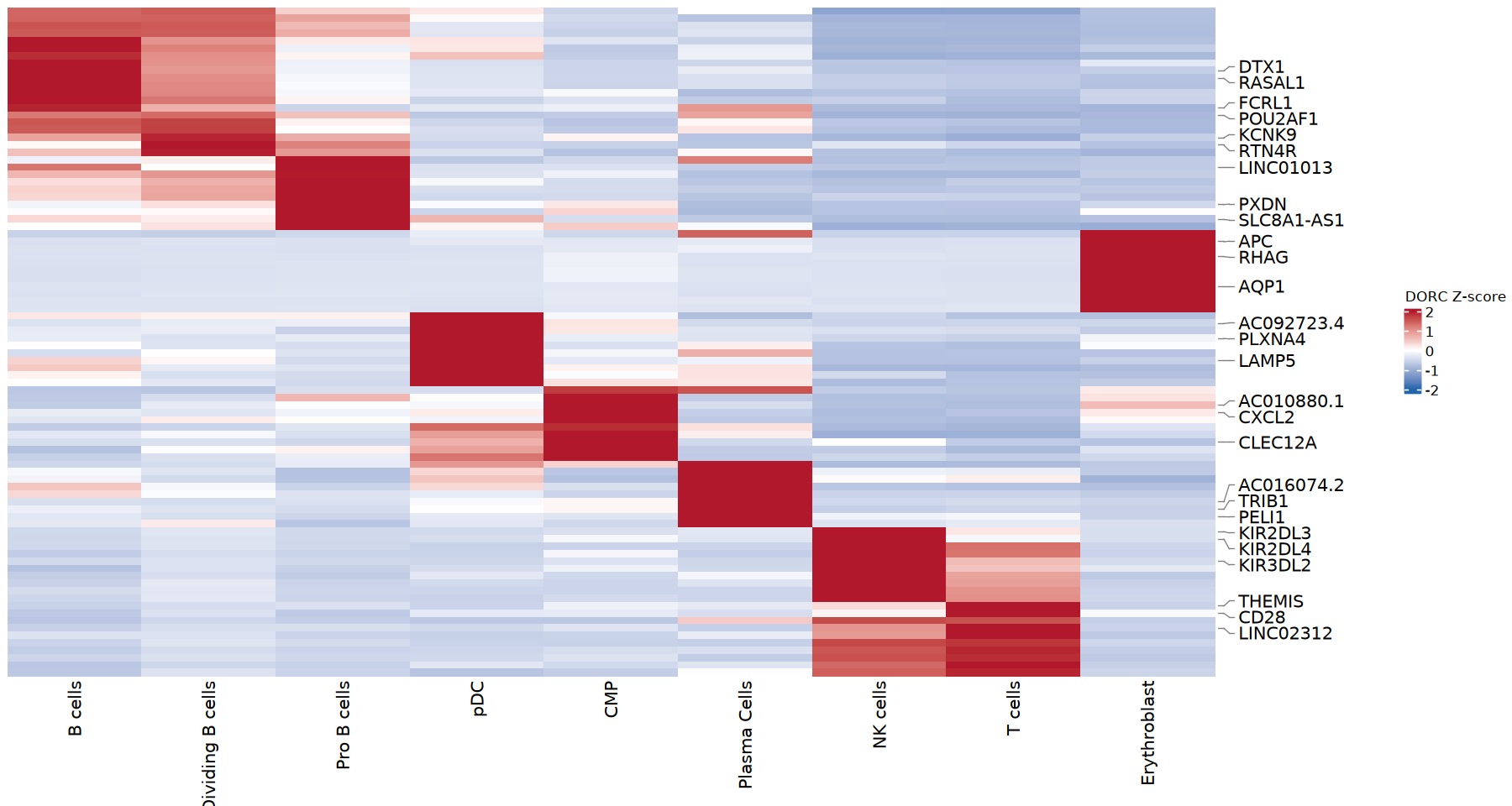

💡 Interpretation Guide: DORC Gene Activity Clustering Heatmap

This heatmap displays the global activity landscape of subpopulation-specific core DORC genes. Data have been aggregated at the cell-population level (Pseudobulk averaging), and gene activities have been Z-score row-normalized.

• Y-axis (Rows): Represents the Top 10 most significant differential DORC genes extracted from each cell subpopulation, ranked by avg_log2FC. The dendrogram on the left reflects the similarity clustering of these genes in global regulatory patterns.
• X-axis (Columns): Represents the different cell subpopulations defined in the data. The dendrogram on the columns reflects the phylogenetic relationships among cell subpopulations at the core regulatory network level.
• Color Gradient (Z-score): Reflects the relative regulatory activity of a specific gene across different cell populations.
  • Red: Indicates that the activity of this DORC gene in this cell population is significantly higher than the average.
  • Blue: Indicates activity significantly below average.
  • White: Indicates close to the average.
• Core Findings: By inspecting the "red highlighted block matrix" on the heatmap, one can intuitively pinpoint the core transcriptional regulatory hubs driving the development of specific cell lineages or maintaining their biological characteristics.