
ATAC + RNA Multi-omics: Differential Accessibility Analysis
1. Tutorial Overview
This tutorial leverages single-cell multi-omics analysis tools including Seurat + Signac + clusterProfiler, and is designed to perform differential Peak analysis, Peak-to-nearest-gene annotation, and downstream functional interpretation on SeekArc single-cell multi-omics data (RNA + ATAC).
This tutorial is intended for SeekArc multi-omics data that have already undergone dimensionality reduction and clustering. By identifying differentially accessible chromatin regions (differential peaks) between cell populations or experimental conditions, and combining ClosestFeature() for nearest-gene annotation, it maps epigenome-level chromatin accessibility changes onto potential target genes, achieving the following core analytical objectives:
- Identifying Cell-Type-Specific Accessible Chromatin Regions: Detect open peaks specific to different cell clusters, assisting in cell identity definition;
- Mining Condition-Specific Regulatory Elements: Compare differential peaks across different treatment groups or disease groups, revealing chromatin remodeling events under environmental stimuli or pathological states;
- Target Gene Prediction for Differential Peaks: Associate differential peaks with putatively regulated genes using the nearest-neighbor rule, providing epigenome-dimensional supplementary evidence for downstream RNA-level differential expression analysis;
- Enrichment Analysis and Biological Pathway Mining: Feed the annotated list of nearest genes into
clusterProfilerto perform GO/KEGG and other functional enrichment analyses, revealing the biological processes in which differentially accessible regions participate.
💡 The figures shown in the documentation represent only a subset of representative visualizations. For the complete analysis results across all cell populations or comparison groups (including detailed data tables and all high-resolution plots), please refer to the
../result/directory.
suppressPackageStartupMessages(suppressWarnings({
    library(presto)
    library(ggrepel)
    library(Seurat)
    library(BiocGenerics)
    library(S4Vectors)
    library(IRanges)
    library(Signac)
    library(ComplexHeatmap)
    library(Biobase)
    library(AnnotationDbi)
    library(org.Hs.eg.db)
    library(org.Mm.eg.db)
    library(GenomicRanges)
    library(JASPAR2020)
    library(TFBSTools)
    library(memuse)
    library(stringr)
    library(dplyr)
    library(DOSE)
    library(clusterProfiler)
    library(enrichplot)
    library(foreach)
    library(doParallel)
    library(base64enc)
    library(DT)
    library(KEGG.db)
}))if (requireNamespace("future", quietly = TRUE)) {
cores <- parallelly::availableCores()
workers <- as.integer(floor(cores * 0.7))
if (.Platform$OS.type == "unix") {
future::plan(future::multicore, workers = workers)
} else {
future::plan(future::multisession, workers = workers)
}
message("total cores =", cores, ",uses ", workers, " works")
}
if (requireNamespace("memuse", quietly = TRUE)) {
total_mem <- memuse::Sys.meminfo()$totalram
total_mem_bytes <- as.numeric(total_mem)
future_mem <- total_mem_bytes * 0.7
future_mem_gb <- future_mem / 1024^3
total_mem_gb <- total_mem_bytes / 1024^3
} else {
future_mem <- 50 * 1024^3
future_mem_gb <- 50
total_mem_gb <- 50 / 0.6
}
options(future.globals.maxSize = future_mem)2. Input File Preparation
2.1 Input File Requirements
This tutorial primarily performs advanced differential analysis (DiffEnrich) based on a pre-processed Seurat multi-omics object. Before starting, the following core input files need to be prepared:
input.rds: The pre-processed Seurat object file. This object must contain bothRNAandATACassays, and the ATAC modality must have already undergone basic Peak calling.meta.tsv: Cell metadata file (tab-separated). Must contain abarcodecolumn, as well as columns defining cell type (e.g.,Celltype) and sample grouping (e.g.,Sample).genome.fa: Reference genome FASTA file for the corresponding species. Used downstream to extract DNA sequences from ATAC peaks for Motif matching and ChromVAR TF activity scoring.- ATAC fragment file and index: The
fragments.tsv.gzand its.tbiindex file required for constructing the ATAC Assay. Please ensure these files are stored in the designated output directory (or consistent with the path configured in the script) so that Signac can read them correctly.
Example Directory Structure
It is recommended to organize your input data and metadata according to the following structure:
PBMC_demo/
├── input.rds                  # Seurat object containing scRNA and scATAC data
├── meta.tsv                   # Metadata table containing cell type and grouping information
├── genome.fa                  # Reference genome sequence file (e.g., hg38.fa)
└── fragments/                 # Location of ATAC fragment files
    ├── sample1_fragments.tsv.gz
└── sample1_fragments.tsv.gz.tbi# --- Input Parameter Configuration --- Fill in parameters here according to your own needs
## fpath: Directory where fragment files are located
fpath = "/path/to/fpath"
## rds: Path to the input Seurat object RDS file, containing pre-processed single-cell multi-omics data
rds = "/path/to/input.rds"
## meta: Metadata file path (TSV format), containing sample information, cell-type annotations, and other metadata
meta = "/path/to/meta.tsv"
## species: Species information; "others" indicates a non-standard model organism (species other than human/mouse)
species = "human"
## clusters_col: Column name in the metadata used to identify cell type / clustering
clusters_col = "Celltype"
## celltypes: List of cell types to be analyzed; multiple cell types separated by commas
celltypes = "B cells,CMP,Dividing B cells,Erythroblast,NK cells,pDC,Plasma Cells,Pro B cells,T cells"
## downsample: Whether to perform cell downsampling; TRUE enables downsampling to balance cell counts across cell types
downsample = "TRUE"
## downsample_num: Target cell count after downsampling; maximum number of cells retained per cell type
downsample_num = "3000"
## group_comparison: Column name in the metadata used for group comparison; typically sample grouping or treatment condition
group_comparison = "Sample"
## case_group: Group name for the experimental / case group, used for differential enrichment analysis
case_group = "XYRD_pbmc_2_arc"
## control_group: Group name for the control group, used for differential enrichment analysis
control_group = "25030508_pbmc_1_arc"
## logFC: Log fold change threshold, used to filter significantly differential features
logFC = "0.25"
## pval_adj: Adjusted p-value threshold, used for statistical significance testing
pval_adj = "0.05"group_colors <- c(
"#F7E55C",
"#F08080"
)
names(group_colors) <- c(case_group, control_group)
pseudobulk_size <- 5
output <- "../result"
celltypes <- strsplit(celltypes,",")[[1]]
downsample_num <- as.numeric(downsample_num)
logFC <- as.numeric(logFC)
pval_adj <- as.numeric(pval_adj)dir.create(paste0(output,'/DIFF/01_diffPeak'), recursive = TRUE)
dir.create(paste0(output,'/DIFF/02_topPeak'), recursive = TRUE)
dir.create(paste0(output,'/DIFF/03_closestFeature'), recursive = TRUE)2.2 Function Definitions
Before commencing the analysis, several core helper functions need to be pre-defined for efficient repeated invocation in subsequent analysis loops. The script mainly defines the following three functional functions:
make_pseudobulkFunction Its purpose is to aggregate the sparse single-cell matrix into pseudobulk form according to the specified grouping and size (pb_size), reducing the sparsity of single-cell data and thereby improving the robustness of downstream correlation computation and heatmap visualization.go_enrichFunction This function primarily uses theenrichGOfunctionality of theclusterProfilerpackage to perform GO (Gene Ontology) enrichment analysis on input target genes (in Symbol format). The analysis covers three aspects: Biological Process (BP), Cellular Component (CC), and Molecular Function (MF) (ont='ALL'). In addition to outputting a complete enrichment result table (.xls), the function also automatically generates a barplot and dotplot displaying the Top 20 significantly enriched pathways, with automatic line-wrapping applied to overly long pathway names during plotting to ensure aesthetic layout.kegg_enrichFunction This function is responsible for executing KEGG pathway enrichment analysis. Since the KEGG database requires ENTREZID as input, the function internally performs gene ID mapping first and calls the online KEGG database (use_internal_data = FALSE) for enrichment computation. To improve result readability, the function has built-in result cleaning logic: it strips redundant species suffix information from pathway descriptions and converts the ENTREZID in enrichment results back into readable Symbol gene names, finally exporting detailed result tables along with corresponding barplots and dotplots.
make_pseudobulk <- function(mat, groups, pb_size = 10) {
    mat <- as.matrix(mat)
    groups <- as.character(groups)
    stopifnot(ncol(mat) == length(groups))
    if (!is.numeric(pb_size) || length(pb_size) != 1 || is.na(pb_size)) {
        stop("pb_size must be single number")
    }
    pb_size <- as.integer(pb_size)
    if (pb_size < 1) pb_size <- 1L

    pb_cols <- list()
    pb_group <- character(0)
    pb_names <- character(0)

    grp_levels <- unique(groups)
    for (g in grp_levels) {
        idx <- which(groups == g)
        if (length(idx) == 0) next

        # such as pb_size=10: 1-10 -> pb1, 11-20 -> pb2 ...
        split_id <- ((seq_along(idx) - 1L) %/% pb_size) + 1L
        chunk_list <- split(idx, split_id)

        for (j in seq_along(chunk_list)) {
            cidx <- chunk_list[[j]]
            if (length(cidx) == 1) {
                pb_vec <- as.numeric(mat[, cidx, drop = TRUE])
            } else {
                pb_vec <- rowMeans(mat[, cidx, drop = FALSE])
            }
            pb_cols[[length(pb_cols) + 1L]] <- pb_vec
            pb_group <- c(pb_group, g)
            pb_names <- c(pb_names, paste0(g, "_pb", j))
        }
    }
    if (length(pb_cols) == 0) {
        pb_mat <- matrix(numeric(0), nrow = nrow(mat), ncol = 0)
        rownames(pb_mat) <- rownames(mat)
        return(list(mat = pb_mat, group = character(0), pb_names = character(0)))
    }

    pb_mat <- do.call(cbind, pb_cols)
    colnames(pb_mat) <- make.unique(pb_names)
    rownames(pb_mat) <- rownames(mat)

    list(mat = pb_mat, group = pb_group, pb_names = colnames(pb_mat))
}go_enrich <- function(eg,db,outdir,prefix) {
genelist <- eg$SYMBOL
go <- enrichGO(genelist, OrgDb=db, ont='ALL',pAdjustMethod = 'BH',qvalueCutoff = 1,pvalueCutoff = 1,keyType = 'SYMBOL')
go1 <- data.frame(cluster=prefix, go)
write.table(go1,file=paste(outdir,'/',prefix,'_GOenrich.xls',sep=''),sep='\t',quote=F,row.names=F)
pdf(paste0(outdir,'/',prefix,'_GO_bar.pdf',sep=''),width = 8, height = 8)
print(barplot(go,showCategory=20,drop=T)+ scale_y_discrete(labels = function(x) str_wrap(x, width = 50)))
dev.off()
pdf(paste0(outdir,'/',prefix,'_GO_dot.pdf',sep=''),width = 8, height = 8)
print(dotplot(go,showCategory=20)+ scale_y_discrete(labels = function(x) str_wrap(x, width = 50)))
dev.off()
}kegg_enrich <- function(eg, species, outdir, prefix) {
genenames <- eg$SYMBOL
names(genenames) <- eg$ENTREZID
genelist <- eg$ENTREZID
kegg <- enrichKEGG(
gene = genelist,
organism = species, # bta
keyType = "kegg",
pAdjustMethod = "BH",
pvalueCutoff = 1,
qvalueCutoff = 1,
use_internal_data = FALSE
)
gene_list <- strsplit(kegg$geneID, split = "/")
geneName <- unlist(lapply(gene_list, function(x) paste(genenames[x], collapse = "/")))
kegg@result$Description <- sub("\\s+-\\s+[^\\(]+\\s*\\([^)]+\\)\\s*$", "",
as.character(kegg@result$Description))
KEGGenrich <- data.frame(
cluster = prefix,
kegg[, 1:6],
kegg[, 10:12],
geneName,
kegg[, 14, drop = FALSE]
)
write.table(
KEGGenrich,
file = paste0(outdir, "/", prefix, "_KEGGenrich.xls"),
sep = "\t", quote = FALSE, row.names = FALSE
)
pdf(paste0(outdir, "/", prefix, "_KEGG_dot.pdf"), width = 8, height = 8)
print(dotplot(kegg, showCategory = 20) +
scale_y_discrete(labels = function(x) str_wrap(x, width = 50)))
dev.off()
pdf(paste0(outdir, "/", prefix, "_KEGG_bar.pdf"), width = 8, height = 8)
print(barplot(kegg, showCategory = 20) +
scale_y_discrete(labels = function(x) str_wrap(x, width = 50)))
dev.off()
}3. Data Loading and Preprocessing
Before performing differential Peak analysis, the Seurat object and metadata must be loaded first, and the target cell populations must be extracted, filtered, and downsampled according to analysis needs, to ensure the accuracy and statistical validity of subsequent comparisons.
3.1 Loading the Seurat Object and Metadata
First, read the input .rds object. If a separate metadata file (meta.tsv) is provided, the program reads it and merges it into the Seurat object, providing the basis for subsequent group comparisons (e.g., case_group vs control_group) and cell-type identification (clusters_col).
obj <- readRDS(rds)
if (meta != ""){
  meta <- read.table(meta,header=T,sep='\t',check.names=F)
  rownames(meta) <- meta$barcode
  obj <- AddMetaData(obj, meta)
}
obj <- subset(obj, subset = !!sym(clusters_col) %in% celltypes)
DefaultAssay(obj) <- "ATAC"
Idents(obj) <- clusters_col
💡 NoteNote: The
barcodeinmeta.tsvmust be exactly identical to the cell names (colnames) of the Seurat object ininput.rds.
3.2 Cell Type Selection and Downsample Balancing
To avoid statistical bias caused by overly abundant cell types in the analysis, the program provides cell-type extraction and downsampling functions:
- Selecting Target Cells: Based on the
celltypesparameter, retain only cell types of interest (e.g.,B cells, T cells, etc.). - Performing Downsampling: When
downsample = TRUEis enabled, the program randomly samples each cell type, limiting the cell count to withindownsample_num(e.g., 3000), thereby balancing cell numbers across different cell types.
if (downsample == 'TRUE'){
    print(levels(Idents(obj)))
    Idents(obj) <- clusters_col
    obj <-subset(obj, downsample = downsample_num)
    print('downsample')
    print(dim(obj@meta.data))
}
3.3 Correcting Fragment File Paths
When transferring single-cell objects or reading across servers, the fragment file paths in the ATAC modality frequently become invalid. The program iterates through all Fragment records of the ATAC Assay in the Seurat object, extracts the file names, and redirects their paths to the current output directory (fpath), ensuring that subsequent operations requiring underlying sequences — such as computing TSS enrichment and drawing CoveragePlots — can locate files correctly.
n_fragments <- length(obj@assays$ATAC@fragments)
for (i in 1:n_fragments) {
  original_path <- obj@assays$ATAC@fragments[[i]]@path
  filename <- basename(original_path)
  obj@assays$ATAC@fragments[[i]]@path <- paste0(fpath, '/', filename)
}
4. Starting Differential Peak Analysis
4.1 Differential Peak Identification Across Cell Populations / Groups
The wilcoxauc function from the presto package is faster and more efficient for differential Peak analysis compared to Seurat's FindAllMarkers and FindMarkers. Therefore, this tutorial uses the Wilcoxon rank-sum test to perform differential analysis on the accessibility matrix of the ATAC Assay.
Depending on the analytical objective, two differential analysis modes are generally available.
- Single-Cluster Marker Identification Mode (Cluster vs All)
- Trigger Condition: When the
group_comparisonparameter is empty (""). - Analysis Logic: The program compares every cell type (or cluster) in the dataset against all remaining cells. This mode is primarily used to identify the exclusive open regions (Cluster-specific Marker Peaks) that define a particular cell type (e.g., B cells, T cells).
- Trigger Condition: When the
- Intra-Cell-Type Group Difference Mode (Case vs Control)
- Trigger Condition: When the
group_comparisonparameter is not empty (e.g., set to"Sample"). - Analysis Logic: The program first extracts the two groups specified for comparison (
case_groupandcontrol_group), then iterates through every cell type, comparing disease group (experimental group) versus control group within each cell type. - Application Scenarios: This mode is commonly used to explore specific epigenetic changes in particular cell subpopulations under disease occurrence, drug treatment, or different developmental stages. After computation, the program merges all intra-cell-type group difference results into a master table (
all_diffPeak.xls) and exports it automatically.
- Trigger Condition: When the
This tutorial will select which analysis mode to execute based on whether the group_comparison parameter is empty.
if (group_comparison == "") {
    da_peaks <- wilcoxauc(obj, clusters_col, assay='data', seurat_assay='ATAC')
    colnames(da_peaks)[2] <- 'cluster'
} else {
    all_da_peaks <- list()
    obj <- subset(obj, subset = !!sym(group_comparison) %in% c(case_group, control_group))

    for (cell_type_analyse in unique(obj@meta.data[[clusters_col]])) {
        tryCatch({
            sub_obj <- subset(obj, subset = !!sym(clusters_col) %in% cell_type_analyse)
            da_peaks <- wilcoxauc(sub_obj,
                                        group_by = group_comparison,
                                        assay = 'data',
                                        seurat_assay = 'ATAC',
                                        groups_use = c(case_group, control_group))
            da_peaks$cluster <- as.character(cell_type_analyse)
            all_da_peaks[[as.character(cell_type_analyse)]] <- da_peaks
        }, error = function(e) {
        message(sprintf("Error in cluster %s: %s", cell_type_analyse, e$message))
        })
    }
    da_peaks <- do.call(rbind, all_da_peaks)

    write.table(da_peaks,
               file = paste0(output, '/DIFF/all_diffPeak.xls'),
               quote = F, row.names = F, col.names = T, sep = '\t')
}head(da_peaks[da_peaks$padj < pval_adj & da_peaks$logFC > logFC, ])| feature | group | avgExpr | logFC | statistic | auc | pval | padj | pct_in | pct_out | cluster | |
|---|---|---|---|---|---|---|---|---|---|---|---|
| <chr> | <chr> | <dbl> | <dbl> | <dbl> | <dbl> | <dbl> | <dbl> | <dbl> | <dbl> | <chr> | |
| T cells.130 | chr1-1692209-1693568 | 25030508_pbmc_1_arc | 0.7942903 | 0.3801981 | 777228.5 | 0.6371901 | 2.159255e-29 | 6.461503e-26 | 50.927835 | 31.8489066 | T cells |
| T cells.1059 | chr1-12510125-12511334 | 25030508_pbmc_1_arc | 0.4425744 | 0.2932666 | 658140.5 | 0.5395589 | 2.695462e-12 | 6.892835e-10 | 11.958763 | 4.2544732 | T cells |
| T cells.2161 | chr1-25774578-25775743 | 25030508_pbmc_1_arc | 0.4612178 | 0.2908842 | 689600.5 | 0.5653506 | 4.535117e-18 | 3.051895e-15 | 20.618557 | 8.2703777 | T cells |
| T cells.4675 | chr1-59814184-59815421 | 25030508_pbmc_1_arc | 0.4529309 | 0.3608838 | 687916.5 | 0.5639700 | 3.876126e-28 | 9.912029e-25 | 16.288660 | 3.8170974 | T cells |
| T cells.4936 | chr1-64876900-64877760 | 25030508_pbmc_1_arc | 0.3995816 | 0.2821482 | 649553.0 | 0.5325187 | 1.865536e-11 | 3.864215e-09 | 9.278351 | 2.9423459 | T cells |
| T cells.5445 | chr1-83508232-83508942 | 25030508_pbmc_1_arc | 0.2853563 | 0.2793229 | 640625.0 | 0.5251993 | 4.262219e-26 | 8.347758e-23 | 5.154639 | 0.1192843 | T cells |
💡 Interpretation Guide
The above table interactively displays the differential Peak result table. Each row represents a differential accessibility Peak, used to answer "which group is more open at this Peak, what is the significance, and what is the effect size."
- feature: Peak coordinates (e.g.,
chr1-4846826-4847624), i.e., the peak with differential accessibility.- group: Group information, indicating that this Peak is more open in this group; this column appears only in inter-group differential analysis.
- cluster: Cell population name, indicating in which specific cell population this Peak shows differential accessibility.
- avgExpr: Average accessibility level of this Peak in the target group — it is the mean ATAC signal; larger values typically indicate overall higher openness.
- logFC: Log-fold-change effect size — the value after log transformation of the fold change; the larger the positive value, the larger the fold change.
- statistic: Wilcoxon test statistic, used for ranking and significance computation.
- auc: Discrimination metric; 0.5 approximates no difference, with greater deviation from 0.5 indicating stronger discriminative ability.
- pval: Raw P-value, indicating differential significance.
- padj: P-value after multiple-testing correction; typically used as the primary metric for significance judgment.
- pct_in: Percentage of cells in the target group where this Peak's signal is detectable.
- pct_out: Percentage of cells in the control group / remaining groups where this Peak's signal is detectable; comparing with
pct_inprovides an intuitive view of inter-group coverage differences.
saveRDS(obj,paste0(output, '/output.rds'))
write.table(da_peaks[da_peaks$padj < pval_adj & da_peaks$logFC > logFC, ],paste0(output,'/DIFF/01_diffPeak/all_diffPeak_significant.xls'),quote=F,row.names=F,col.names=T,sep='\t')
4.2 CoveragePlot Visualization of Differential Peaks
Purely statistical tables (e.g., p-value and logFC) can identify significantly changed regions, but cannot intuitively reflect the true chromatin accessibility state. To verify the reliability of statistical results and intuitively display epigenetic differences, we need to return to the raw sequencing data level for inspection.
The following code module iterates through each cell cluster (Cluster), performing deep visualization of its significant differential Peaks:
- Extracting Top Candidate Regions: After filtering with stringent significance thresholds, the program sorts by effect size (
logFC) in descending order and automatically extracts the Top differential Peaks with the most dramatic changes. - Plotting Chromatin Coverage Plots: Call Signac's
CoveragePlotfunction, centered on the extracted Top Peak coordinates, extending 5000 bp upstream and downstream. This plot extracts and overlays the Tn5 transposase insertion fragment signals of the selected cell populations in the experimental group versus the control group (or other cell populations), generating an intuitive genomic Track plot.
Through CoveragePlot, we can clearly observe the height changes of the "Peak" patterns in specific genomic intervals across different comparison groups, providing the most direct biological visual evidence for our differential statistical results.
cluster <- unique(da_peaks$cluster)

sort_clusters <- function(x) {
  if(all(!is.na(suppressWarnings(as.numeric(x))))) {
    return(x[order(as.numeric(x))])
  } else {
    nums <- suppressWarnings(as.numeric(gsub("[^0-9]", "", x)))
    if(all(!is.na(nums))) {
      return(x[order(nums)])
    } else {
      return(sort(x))
    }
  }
}
cluster <- sort_clusters(cluster)for (i in cluster) {
tryCatch({
DefaultAssay(obj) <- "ATAC"
data <- da_peaks[da_peaks$cluster == i, ]
valid_rows <- grepl("^([^-]+)-(\\d+)-(\\d+)$", data$feature)
if (sum(!valid_rows) > 0) {
data <- data[valid_rows, ]
}
if (group_comparison == "") {
analysis_groups <- c("cluster_marker")
} else {
analysis_groups <- c(case_group, control_group)
}
for (grp in analysis_groups) {
tryCatch({
if (grp == "cluster_marker") {
data.sig <- data[data$padj < pval_adj & data$logFC > logFC, ]
prefix <- paste0('c_', gsub(" ", "", i))
} else {
data.sig <- data[data$group == grp & data$padj < pval_adj & data$logFC > logFC, ]
prefix <- paste0('c_', gsub(" ", "", i), '_', gsub(" ", "", grp))
}
if (nrow(data.sig) == 0) next
peaks.top <- head(data.sig[order(data.sig$logFC, decreasing = TRUE), ])[['feature']]
if (length(peaks.top) > 0) {
print(paste0("Drawing CoveragePlot for Top Peak in ", prefix, ": ", peaks.top[1]))
if (group_comparison == "") {
p_cov <- CoveragePlot(
object = obj,
region = peaks.top[1],
extend.upstream = 5000,
extend.downstream = 5000,
nrow = 1
)
} else {
p_cov <- CoveragePlot(
object = obj,
region = peaks.top[1],
extend.upstream = 5000,
extend.downstream = 5000,
nrow = 1,
group.by = group_comparison,
idents = c(case_group, control_group)
)
}
print(p_cov)
ggsave(paste0(output, '/DIFF/02_topPeak/', prefix, '_diffPeak_top.pdf'),
p_cov, width = 24, height = 3)
}
}, error = function(e) {
message(sprintf("Error drawing CoveragePlot for cluster %s, group %s: %s", i, grp, e$message))
})
}
}, error = function(e) {
message(sprintf("Error processing cluster %s: %s", i, e$message))
})
}options(repr.plot.width = 10, repr.plot.height = 4)
p_cov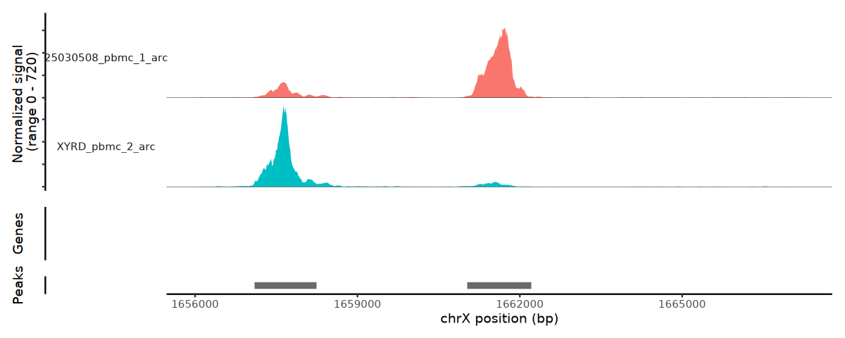
💡 Note
This example plot displays the ATAC coverage signal differences of one set of Top differential Peaks across different groups or clusters. Each small panel corresponds to the region around a candidate key Peak; by comparing the peak heights and shapes across multiple tracks above and below, one can verify whether the statistical differences are visible at the raw signal level.
- Top / Bottom Tracks: Normalized ATAC coverage signals of two groups or multiple cell clusters in the same region; the higher the peak, the stronger the accessibility in that region.
- Normalized signal: The y-axis represents normalized coverage intensity, allowing comparison of relative heights between two groups within the same panel.
- chr position (bp): The x-axis shows genomic coordinates, displaying this Peak and its upstream/downstream neighborhood.
- Genes Track: Shows the structure and orientation of neighboring genes, facilitating judgment of which functional genes the differential Peak may affect.
- Peak Markers: Short gray bars represent called open regions; focus on whether the position of the Top differential Peak is consistent with inter-group signal changes.
- Multi-Panel Side-by-Side: Each panel shows one Top peak locus, facilitating rapid screening of high-confidence candidate regions that are "statistically significant and also clearly separated in the image."
4.3 Global Differential Peak Heatmap Display
Use ComplexHeatmap to plot a heatmap, displaying the signal changes of specifically accessible regions from a panoramic perspective:
Data Smoothing and Normalization Extract the Top 500 differential Peaks from each group for Pseudobulk aggregation, and enhance contrast via Z-score normalization to avoid excessive sparsity at the single-cell level.
Dual Display Modes According to the analysis strategy, automatically generate either the "All-Cluster Marker Master Heatmap" (distinguishing different cell populations) or the "Specific-Cell-Type Inter-Group Difference Heatmap" (comparing experimental group versus control group).
Precise Top Peak Annotation Dynamically extract the coordinates of the Top 5 most significant differential Peaks ranked in each group, using
anno_markfunctionality for precise connecting-line annotation on the right side of the heatmap, helping to quickly locate the core genomic regions with the most dramatic changes.
tryCatch({
    ensure_color_map <- function(values, color_map) {
        values <- unique(as.character(values))
        values <- values[!is.na(values)]
        if (!all(values %in% names(color_map))) {
            miss <- setdiff(values, names(color_map))
            if (length(miss) > 0) {
                extra_cols <- setNames(scales::hue_pal()(length(miss)), miss)
                color_map <- c(color_map, extra_cols)
            }
        }
        color_map
    }

    if (group_comparison == "") {
        all_top_peaks <- c()
        peak_cluster_anno <- c()

        mark_peaks_list <- list()

        for (i in cluster) {
            data.sig <- da_peaks[da_peaks$cluster == i & da_peaks$padj < pval_adj & da_peaks$logFC > logFC, ]
            if (nrow(data.sig) > 0) {
                data.sig <- data.sig[order(data.sig$logFC, decreasing = TRUE), ]
                top_n <- min(nrow(data.sig), 500)
                sel_peaks <- data.sig$feature[1:top_n]

                all_top_peaks <- c(all_top_peaks, sel_peaks)
                peak_cluster_anno <- c(peak_cluster_anno, rep(i, top_n))

                top5_peaks <- head(sel_peaks, 5)
                mark_peaks_list[[as.character(i)]] <- top5_peaks
            }
        }

        if (length(all_top_peaks) > 0) {
            cell_order <- order(factor(obj@meta.data[[clusters_col]], levels = cluster))
            cells_use <- rownames(obj@meta.data)[cell_order]

            DefaultAssay(obj) <- "ATAC"
            mat <- GetAssayData(obj, assay = "ATAC", slot = "data")[all_top_peaks, cells_use, drop = FALSE]
            mat <- as.matrix(mat)

            cluster_vec <- as.character(obj@meta.data[cells_use, clusters_col, drop = TRUE])
            pb <- make_pseudobulk(mat = mat, groups = cluster_vec, pb_size = pseudobulk_size)
            mat <- pb$mat
            col_df <- data.frame(Cluster = pb$group, row.names = colnames(mat), stringsAsFactors = FALSE)

            mat_scaled <- t(scale(t(mat)))
            mat_scaled[is.na(mat_scaled)] <- 0
            mat_scaled[mat_scaled > 2] <- 2
            mat_scaled[mat_scaled < -2] <- -2

            cols_use <- ensure_color_map(col_df$Cluster, group_colors)

            col_anno <- HeatmapAnnotation(
                df = col_df,
                col = list(Cluster = cols_use),
                show_annotation_name = FALSE
            )


            target_peaks <- unlist(mark_peaks_list)
            target_idx <- match(target_peaks, rownames(mat_scaled))

            valid_idx <- !is.na(target_idx)
            mark_at <- target_idx[valid_idx]
            mark_labels <- target_peaks[valid_idx]

            right_anno <- rowAnnotation(
                Peaks = anno_mark(
                    at = mark_at,
                    labels = mark_labels,
                    which = "row",
                    side = "right",
                    labels_gp = gpar(fontsize = 8, fontface = "bold", col = "black"),
                    lines_gp = gpar(col = "black", lty = 1),
                    link_width = unit(4, "mm"),
                    padding = unit(0.5, "mm"),
                    extend = unit(c(1, 1), "mm")
                )
            )

            col_fun <- circlize::colorRamp2(
                c(-2, -1, 0, 1, 2),
                c("#2c7bb6", "#abd9e9", "#f7f7f7", "#fdae61", "#d7191c")
            )

            ht <- Heatmap(
                mat_scaled,
                col = col_fun,
                cluster_rows = FALSE,
                cluster_columns = FALSE,
                show_row_names = FALSE,
                show_column_names = FALSE,
                show_row_dend = FALSE,
                row_title_rot = 0,
                top_annotation = col_anno,
                right_annotation = right_anno,
                name = "Accessibility",
                use_raster = TRUE
            )

            pdf(paste0(output, "/DIFF/01_diffPeak/All_Clusters_DiffPeak_Heatmap.pdf"), width = 12, height = 10)
            draw(ht, padding = unit(c(10, 6, 6, 10), "mm"))
            dev.off()
        }
    } else {
        for (i in cluster) {
            data.sig <- da_peaks[da_peaks$cluster == i & da_peaks$padj < pval_adj & da_peaks$logFC > logFC, ]
            if (nrow(data.sig) > 0) {
                sel_peaks <- c()
                peak_group_anno <- c()

                mark_peaks_list <- list()

                for (grp in c(case_group, control_group)) {
                    data.grp <- data.sig[data.sig$group == grp, ]
                    if (nrow(data.grp) > 0) {
                        data.grp <- data.grp[order(data.grp$logFC, decreasing = TRUE), ]
                        top_n <- min(nrow(data.grp), 500)
                        grp_peaks <- data.grp$feature[1:top_n]

                        sel_peaks <- c(sel_peaks, grp_peaks)
                        peak_group_anno <- c(peak_group_anno, rep(grp, top_n))

                        mark_peaks_list[[grp]] <- head(grp_peaks, 5)
                    }
                }

                cells_in_cluster <- rownames(obj@meta.data)[obj@meta.data[[clusters_col]] == i]
                sub_meta <- obj@meta.data[cells_in_cluster, , drop = FALSE]
                cell_order <- order(factor(sub_meta[[group_comparison]], levels = c(case_group, control_group)))
                cells_use <- cells_in_cluster[cell_order]

                if (length(cells_use) > 0 && length(sel_peaks) > 0) {
                    DefaultAssay(obj) <- "ATAC"
                    mat <- GetAssayData(obj, assay = "ATAC", slot = "data")[sel_peaks, cells_use, drop = FALSE]
                    mat <- as.matrix(mat)

                    group_vec <- as.character(sub_meta[cells_use, group_comparison, drop = TRUE])
                    pb <- make_pseudobulk(mat = mat, groups = group_vec, pb_size = pseudobulk_size)
                    mat <- pb$mat
                    col_df <- data.frame(Group = pb$group, row.names = colnames(mat), stringsAsFactors = FALSE)

                    mat_scaled <- t(scale(t(mat)))
                    mat_scaled[is.na(mat_scaled)] <- 0
                    mat_scaled[mat_scaled > 2] <- 2
                    mat_scaled[mat_scaled < -2] <- -2

                    cols_use <- ensure_color_map(col_df$Group, group_colors)

                    col_anno <- HeatmapAnnotation(
                        df = col_df,
                        col = list(Group = cols_use),
                        show_annotation_name = FALSE
                    )

                    target_peaks <- unlist(mark_peaks_list)
                    target_idx <- match(target_peaks, rownames(mat_scaled))

                    valid_idx <- !is.na(target_idx)
                    mark_at <- target_idx[valid_idx]
                    mark_labels <- target_peaks[valid_idx]

                    right_anno <- rowAnnotation(
                        Peaks = anno_mark(
                            at = mark_at,
                            labels = mark_labels,
                            which = "row",
                            side = "right",
                            labels_gp = gpar(fontsize = 6, fontface = "bold", col = "black"),
                            lines_gp = gpar(col = "black", lty = 2, lwd = 0.5),
                            link_width = unit(8, "mm"),
                            padding = unit(1.5, "mm"),
                            extend = unit(c(15, 15), "mm")
                        )
                    )

                    col_fun <- circlize::colorRamp2(
                        c(-2, -1, 0, 1, 2),
                        c("#2c7bb6", "#abd9e9", "#f7f7f7", "#fdae61", "#d7191c")
                    )

                    ht <- Heatmap(
                        mat_scaled,
                        col = col_fun,
                        cluster_rows = FALSE,
                        cluster_columns = FALSE,
                        show_row_names = FALSE,
                        show_column_names = FALSE,
                        show_row_dend = FALSE,
                        row_title_rot = 0,
                        top_annotation = col_anno,
                        right_annotation = right_anno,
                        name = "Accessibility",
                        column_title = paste0("Cluster: ", i),
                        use_raster = TRUE
                    )

                    pdf(paste0(output, "/DIFF/01_diffPeak/c_", gsub(" ", "", i), "_Group_DiffPeak_Heatmap.pdf"), width = 8, height = 7)
                    draw(ht, padding = unit(c(10, 6, 6, 10), "mm"))
                    dev.off()
                }
            }
        }
    }
}, error = function(e) {
    message("Error in drawing heatmaps: ", e$message)
})options(repr.plot.width = 15, repr.plot.height = 7)
draw(ht,padding = unit(c(10, 6, 6, 10), "mm"))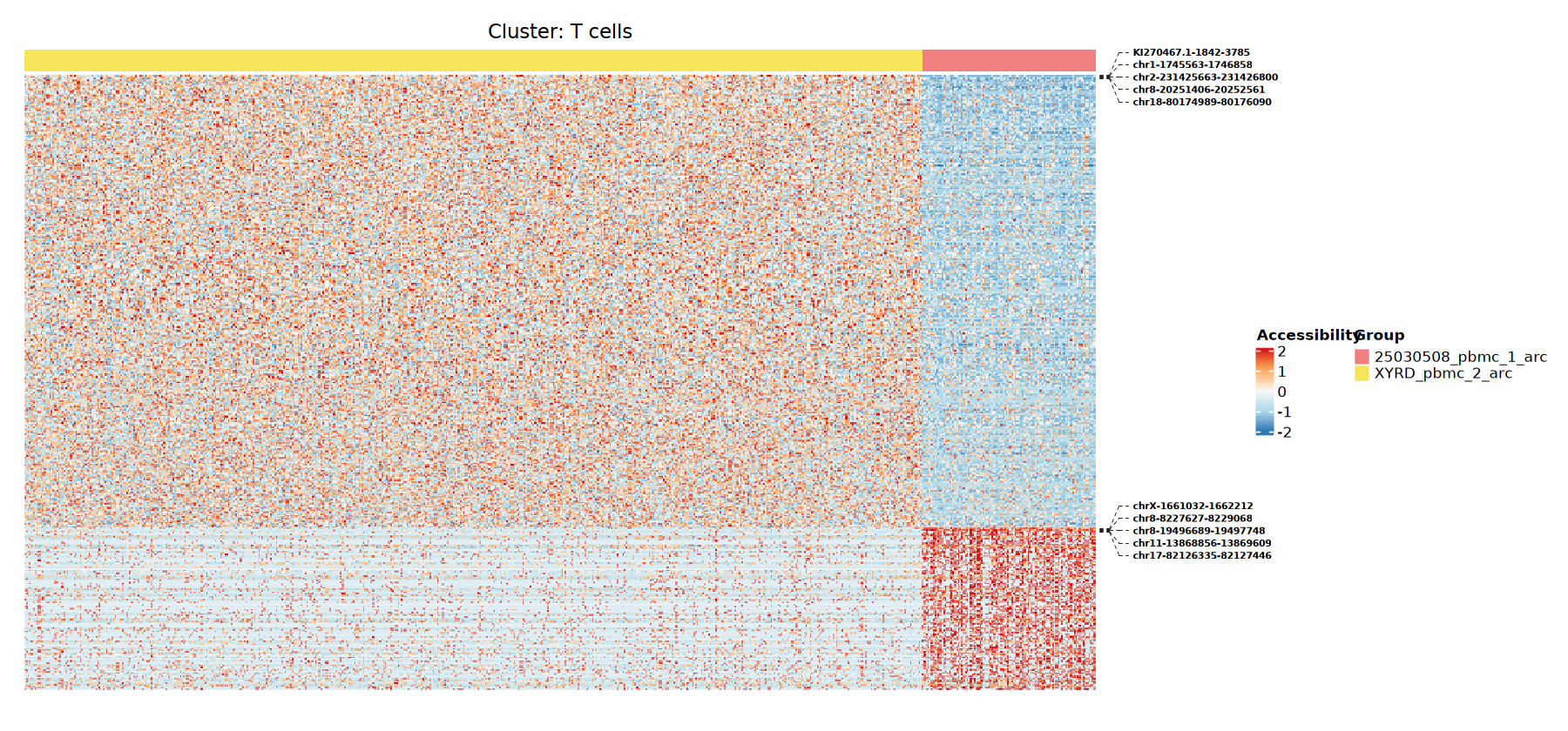
5. Differential Peak Filtering and Nearest-Gene Annotation
5.1 Nearest-Gene Annotation of Differential Peaks
After obtaining the initial differential Peaks across cell populations or experimental groups, the results must be further stringently filtered and biologically annotated, transforming abstract epigenetic signals into concrete gene regulatory clues. For the filtered high-confidence differential Peaks, we can use Signac's ClosestFeature function to precisely map their physical coordinates to the nearest gene on the reference genome. This step directly associates the epigenetic accessibility changes in non-coding regions with the putatively regulated target genes. Annotation results (containing gene name, physical distance, etc.) are output to the 03_closestFeature directory, laying the foundation for subsequent GO/KEGG functional pathway enrichment analysis.
for (i in cluster) {
    tryCatch({
        DefaultAssay(obj) <- "ATAC"
        data <- da_peaks[da_peaks$cluster == i, ]
        valid_rows <- grepl("^([^-]+)-(\\d+)-(\\d+)$", data$feature)
        if (sum(!valid_rows) > 0) {
            message(sprintf("Cluster %s: Removed %d malformed feature rows.", i, sum(!valid_rows)))
            data <- data[valid_rows, ]
        }

        # Determine the groups to iterate over based on group_comparison
        if (group_comparison == "") {
            # Standard single cluster comparison
            analysis_groups <- c("cluster_marker")
        } else {
            # Two group comparison: case and control
            analysis_groups <- c(case_group, control_group)
        }

        for (grp in analysis_groups) {
            print(paste0("Analyzing in progress:", grp))
            tryCatch({

                if (grp == "cluster_marker") {
                    # For single cluster, filter by padj and logFC
                    data.sig <- data[data$padj < pval_adj & data$logFC > logFC, ]
                    prefix <- paste0('c_', gsub(" ", "", i))
                } else {
                    # For group comparison, filter by group and thresholds
                    data.sig <- data[data$group == grp & data$padj < pval_adj & data$logFC > logFC, ]
                    prefix <- paste0('c_', gsub(" ", "", i), '_', gsub(" ", "", grp))
                }

                if (nrow(data.sig) == 0) {
                    message(sprintf("No significant peaks found for %s", prefix))
                    next
                }

                print(dim(data.sig))

                write.table(data.sig, paste0(output, '/DIFF/01_diffPeak/', prefix, '_diffPeak_significant.xls'),
                            quote = FALSE, row.names = FALSE, col.names = TRUE, sep = '\t')


                peaks <- data.sig$feature
                genes <- ClosestFeature(obj, regions = peaks)

                genes$cluster <- as.character(i)
                if (grp != "cluster_marker") {
                    genes$group <- as.character(grp)
                }


                write.table(genes, paste0(output, '/DIFF/03_closestFeature/', prefix, '_diffPeak_sig_genes.xls'),
                            quote = FALSE, row.names = FALSE, col.names = TRUE, sep = '\t')

            }, error = function(e) {
                message(sprintf("Error in cluster %s, group %s: %s", i, grp, e$message))
            })
        }
        print(paste0(i, " Analysis completed."))

    }, error = function(e) {
        message(sprintf("Error in cluster %s: %s", i, e$message))
    })
}data_dir <- paste0(output,"/DIFF/03_closestFeature")
xls_files <- list.files(path = data_dir,
pattern = "diffPeak_sig_genes\\.xls$",
full.names = TRUE)
merged_data <- data.frame()
for (file in xls_files) {
df <- read.table(file, sep="\t", header=TRUE)
df$cluster <- as.character(df$cluster)
merged_data <- bind_rows(merged_data, df)
}
merged_data$cluster <- as.character(merged_data$cluster)
head(merged_data)| tx_id | gene_name | gene_id | gene_biotype | type | closest_region | query_region | distance | cluster | group | |
|---|---|---|---|---|---|---|---|---|---|---|
| <chr> | <chr> | <chr> | <chr> | <chr> | <chr> | <chr> | <int> | <chr> | <chr> | |
| 1 | ENST00000423796 | AC114498.1 | ENSG00000235146 | lncRNA | exon | chr1-594235-594768 | chr1-630357-631124 | 35588 | B cells | 25030508_pbmc_1_arc |
| 2 | ENST00000481276 | SLC35E2B | ENSG00000189339 | protein_coding | exon | chr1-1692449-1692709 | chr1-1692209-1693568 | 0 | B cells | 25030508_pbmc_1_arc |
| 3 | ENST00000650835 | LINC01964 | ENSG00000260840 | lncRNA | exon | chr2-85065895-85067347 | chr2-85089328-85090330 | 21980 | B cells | 25030508_pbmc_1_arc |
| 4 | ENST00000666960 | AL078621.4 | ENSG00000287165 | lncRNA | exon | chr2-113582795-113583152 | chr2-113603235-113604680 | 20082 | B cells | 25030508_pbmc_1_arc |
| 5 | ENST00000440223 | UBE2F | ENSG00000184182 | protein_coding | exon | chr2-237966827-237967132 | chr2-237943150-237943999 | 22827 | B cells | 25030508_pbmc_1_arc |
| 6 | ENST00000453168 | STT3B | ENSG00000163527 | protein_coding | exon | chr3-31532638-31533312 | chr3-31226203-31227780 | 304857 | B cells | 25030508_pbmc_1_arc |
💡 Note The above table displays the results of mapping differential accessible Peaks to the nearest genes (Closest Feature) on the genome. Each row represents a differential Peak and its corresponding putative target gene, used to answer "which gene is most likely regulated by this abnormally open chromatin region."
- tx_id: Transcript ID (e.g.,
ENST00000423796), representing the specific transcript physically closest to this differential Peak.- gene_name: Gene symbol (e.g.,
SLC35E2B), i.e., the commonly used gene name of the transcript mentioned above, facilitating intuitive understanding of gene function.- gene_id: The gene's Ensembl ID (e.g.,
ENSG00000235146), used to uniquely identify this gene.- gene_biotype: The biological type of the gene, e.g.,
protein_coding(protein-coding gene) orlncRNA(long non-coding RNA), helping to judge the nature of the regulatory product.- type: The genomic element type the Peak falls into, e.g.,
exon,intron,promoter, etc.- closest_region: The specific coordinate interval of the reference-annotated element on the genome.
- query_region: The coordinate interval of the Peak we input that shows significant differential accessibility (e.g.,
chr1-630357-631124).- distance: The physical distance (in base pairs, bp) from this differential Peak to the nearest gene element. If the distance is 0, it indicates that this Peak directly overlaps with the target gene.
- cluster: Cell population name, indicating in which specific cell population (e.g.,
B cells) this Peak was identified.- group: Group information, indicating in which comparison group (e.g.,
25030508_pbmc_1_arc) this Peak exhibits specifically high accessibility.
5.2 Functional Annotation of Nearest Genes
After completing the mapping from coordinates to genes, these scattered target genes can be further placed into a macroscopic biological network for examination. By performing GO and KEGG enrichment analysis, we understand what phenotypic changes in the cell are ultimately driven by these regions with altered chromatin accessibility states.
Description of analysis result files in this section: All enrichment analysis results are saved in the 03_closestFeature output directory. For each cell population or comparison group (e.g., prefix), the program automatically generates the following result files:
- Tabular Data: Containing complete enrichment statistical information and corresponding target gene lists (e.g.,
[prefix]_GOenrich.xlsand[prefix]_KEGGenrich.xls). - Visualization Plots: Displaying barplots (
*_GO_bar.pdf,*_KEGG_bar.pdf) and dotplots (*_GO_dot.pdf,*_KEGG_dot.pdf) of the Top 20 significantly enriched pathways respectively, ready for direct use in subsequent reports and presentations.
if (species == "human") {
    kegg_code <- "hsa"
    db <- "org.Hs.eg.db"
    spe <- "human"
} else if (species == "mouse") {
    kegg_code <- "mmu"
    db <- "org.Mm.eg.db"
    spe <- "mouse"
} else {
    stop(paste0("This species is not supported.: '", species,
                "'\nPlease ensure the gene annotation database for the corresponding species has been installed.\n"))
}files <- list.files(paste0(output,"/DIFF/03_closestFeature"),pattern="diffPeak_sig_genes.xls")
for (f in files){
prefix <- gsub('_diffPeak_sig_genes.xls','',f)
f <- paste0(output,"/DIFF/03_closestFeature/",f)
print(f)
print(prefix)
clus_1<-read.table(f,header=T,sep='\t')
clus<-clus_1$gene_name
eg <- NULL
tryCatch({
eg <- bitr(clus, fromType="SYMBOL", toType=c("ENSEMBL","ENTREZID"), OrgDb=db)
print(head(eg))
}, error = function(e) {
message(paste("Processing file ", f, "An error occurred:", e$message))
})
if (is.null(eg) || nrow(eg) == 0) {
message(paste0("Skipping enrichment analysis (no valid mapped genes): ", prefix))
next
}
tryCatch({
go_enrich(eg,db,paste0(output,"/03_closestFeature/clusterProfiler/GO"),prefix)
}, error = function(e) {
message(paste0("GO enrichment analysis failed: ", prefix, " - ", e$message))
})
tryCatch({
kegg_enrich(eg, species, paste0(output,"/03_closestFeature/clusterProfiler/KEGG"), prefix)
}, error = function(e) {
message(paste0("KEGG enrichment analysis failed: ", prefix, " - ", e$message))
})
}go_dir <- paste0(output,"/03_closestFeature/clusterProfiler/GO")
merged_data_go <- data.frame()
if(dir.exists(go_dir)) {
xls_files <- list.files(path = go_dir,
pattern = "\\.xls$",
full.names = TRUE)
for (file in xls_files) {
df <- read.table(file, sep="\t", header=TRUE, fill=TRUE, quote="", check.names=FALSE)
merged_data_go <- bind_rows(merged_data_go, df)
}
if (nrow(merged_data_go) > 0) {
write.table(merged_data_go,
file = file.path(go_dir, "all_GOenrich.xls"),
row.names = FALSE,
sep="\t",
quote=FALSE)
}
}head(merged_data_go)| cluster | ONTOLOGY | ID | Description | GeneRatio | BgRatio | RichFactor | FoldEnrichment | zScore | pvalue | p.adjust | qvalue | geneID | Count | |
|---|---|---|---|---|---|---|---|---|---|---|---|---|---|---|
| <chr> | <chr> | <chr> | <chr> | <chr> | <chr> | <dbl> | <dbl> | <dbl> | <dbl> | <dbl> | <dbl> | <chr> | <int> | |
| 1 | c_Bcells | BP | GO:0030098 | lymphocyte differentiation | 101/1678 | 432/18805 | 0.2337963 | 2.620107 | 10.662915 | 7.040828e-20 | 4.066782e-16 | 3.474463e-16 | PRKCZ/PLA2G2D/ARID1A/PIK3R3/SEMA4A/NTRK1/CD1D/SLAMF6/LY9/PTPRC/HLX/SP3/ITGA4/DOCK10/INPP5D/HDAC4/PLCL2/TGFBR2/CMTM7/CCR9/TLR9/FOXP1/RHOH/AP3B1/FNIP1/IL4/CD74/IRF4/CD83/SOX4/HLA-DRB1/HLA-DOA/RUNX2/PRDM1/FOXO3/TRAF3IP2/VNN1/MYB/ARID1B/CCR6/LFNG/CARD11/ACTB/HDAC9/IKZF1/CDK6/CHD7/TPD52/SMARCA2/IFNA2/PAX5/SHB/SYK/TNFSF8/FUT7/IL2RA/VSIR/ZMIZ1/HHEX/BLNK/RAG2/SPI1/PTPRJ/MS4A1/MEN1/SYVN1/POU2AF1/RNF41/STAT6/USP44/DTX1/ZFP36L1/JAG2/DLL4/CD19/PLCG2/IRF8/ZFPM1/IKZF3/RARA/CCR7/SMARCE1/CD79B/C17orf99/PTPN2/TCF3/AP3D1/CLEC4G/SMARCA4/LYL1/BRD4/IL12RB1/NFKBID/CD79A/CLPTM1/LILRB2/RUNX1/SMARCB1/PATZ1/NFAM1/SASH3 | 101 |
| 2 | c_Bcells | BP | GO:0042113 | B cell activation | 73/1678 | 287/18805 | 0.2543554 | 2.850509 | 9.888159 | 8.608820e-17 | 2.486227e-13 | 2.124113e-13 | LAPTM5/PIK3R3/VAV3/NTRK1/FCRL1/PTPRC/MSH6/SP3/ITGA4/SLC39A10/DOCK10/INPP5D/HDAC4/PLCL2/CMTM7/TLR9/PRKCD/CD38/BANK1/GAPT/MEF2C/FNIP1/IL4/MZB1/CD74/CDKN1A/TNFRSF21/AKIRIN2/TRAF3IP2/CCR6/LFNG/CARD11/HDAC9/LYN/TPD52/IFNA2/PAX5/SHB/SYK/HHEX/BLNK/CD81/SWAP70/RAG2/SPI1/PTPRJ/MS4A1/SYVN1/TBC1D10C/POU2AF1/STAT6/SLC15A4/ZFP36L1/PRKCB/CD19/NOD2/PLCG2/IRF8/IKZF3/CD79B/C17orf99/PTPN2/TCF3/LYL1/CD22/TYROBP/CD79A/ERCC1/SHLD1/NFATC2/TNFRSF13C/NFAM1/SASH3 | 73 |
| 3 | c_Bcells | BP | GO:0050853 | B cell receptor signaling pathway | 33/1678 | 78/18805 | 0.4230769 | 4.741336 | 10.363831 | 3.495526e-15 | 6.730053e-12 | 5.749834e-12 | VAV3/PTPRC/FCMR/IGKC/SLC39A10/PLCL2/FOXP1/KLHL6/CD38/BANK1/MEF2C/SH2B2/BLK/LYN/CD72/SYK/BLNK/CD81/MS4A1/PRKCH/IGHA2/IGHA1/IGHD/PRKCB/CD19/PLCG2/CD79B/CD22/CD79A/NFATC2/MAPK1/IGLC7/NFAM1 | 33 |
| 4 | c_Bcells | BP | GO:0051251 | positive regulation of lymphocyte activation | 74/1678 | 337/18805 | 0.2195846 | 2.460839 | 8.470086 | 2.109515e-13 | 2.769138e-10 | 2.365818e-10 | PRKCZ/ARID1A/VAV3/CD1D/PTPRC/HLX/NCK2/SLC39A10/IGFBP2/INPP5D/TGFBR2/TLR9/HES1/CD38/RHOH/PPP3CA/AP3B1/MEF2C/IL4/CD74/CD83/SOX4/HLA-DRB1/HLA-DQA1/HLA-DOB/HLA-DMB/HLA-DOA/CDKN1A/AKIRIN2/CD24/FOXO3/FYN/VNN1/ARID1B/CARD11/ACTB/LYN/DOCK8/SMARCA2/SHB/SYK/IL2RA/MAP3K8/VSIR/ZMIZ1/IGF2/CD81/SPI1/CCDC88B/STAT6/AKT1/CSK/NOD2/RARA/CCR7/SMARCE1/TCF3/AP3D1/TMIGD2/CD209/SMARCA4/BRD4/FCHO1/IL12RB1/NFKBID/TYROBP/LILRB2/SHLD1/NFATC2/RUNX1/SMARCB1/TNFRSF13C/EFNB1/SASH3 | 74 |
| 5 | c_Bcells | BP | GO:0030217 | T cell differentiation | 72/1678 | 324/18805 | 0.2222222 | 2.490399 | 8.470180 | 2.397107e-13 | 2.769138e-10 | 2.365818e-10 | PRKCZ/PLA2G2D/ARID1A/PIK3R3/SEMA4A/CD1D/SLAMF6/LY9/PTPRC/HLX/SP3/TGFBR2/CCR9/FOXP1/RHOH/AP3B1/IL4/CD74/IRF4/CD83/SOX4/HLA-DRB1/HLA-DOA/RUNX2/PRDM1/FOXO3/TRAF3IP2/VNN1/MYB/ARID1B/CCR6/LFNG/CARD11/ACTB/CDK6/CHD7/SMARCA2/IFNA2/SHB/SYK/TNFSF8/FUT7/IL2RA/VSIR/ZMIZ1/RAG2/SPI1/MEN1/STAT6/USP44/DTX1/ZFP36L1/JAG2/DLL4/ZFPM1/IKZF3/RARA/CCR7/SMARCE1/PTPN2/AP3D1/CLEC4G/SMARCA4/BRD4/IL12RB1/NFKBID/CLPTM1/LILRB2/RUNX1/SMARCB1/PATZ1/SASH3 | 72 |
| 6 | c_Bcells | BP | GO:1903037 | regulation of leukocyte cell-cell adhesion | 81/1678 | 395/18805 | 0.2050633 | 2.298102 | 8.161330 | 7.459736e-13 | 7.181239e-10 | 6.135306e-10 | PRKCZ/PLA2G2D/ARID1A/PTAFR/LAPTM5/CD1D/PTPRC/HLX/NCK2/ITGA4/IGFBP2/TGFBR2/CBLB/HES1/RHOH/PPP3CA/AP3B1/IL4/CD74/DUSP22/CD83/SOX4/RIPOR2/HLA-DRB1/HLA-DQA1/HLA-DOB/HLA-DMB/HLA-DOA/TNFRSF21/CD24/FOXO3/FYN/ARG1/VNN1/ARID1B/MAD1L1/CARD11/ACTB/LYN/DOCK8/SMARCA2/IFNA2/SHB/GCNT1/SYK/FUT7/IL2RA/MAP3K8/VSIR/ZMIZ1/IGF2/CD81/RAG2/CCDC88B/LRRC32/ETS1/WNK1/DTX1/AKT1/CSK/NOD2/RARA/CCR7/SMARCE1/PTPN2/AP3D1/TMIGD2/CLEC4G/CD209/SMARCA4/BRD4/FCHO1/IL12RB1/NFKBID/LILRB2/RUNX1/SMARCB1/ADORA2A/TNFRSF13C/EFNB1/SASH3 | 81 |
kegg_dir <- paste0(output,"/03_closestFeature/clusterProfiler/KEGG")
merged_data_kegg <- data.frame()
if(dir.exists(kegg_dir)) {
    xls_files <- list.files(path = kegg_dir,
                           pattern = "\\.xls$",
                           full.names = TRUE)

    for (file in xls_files) {
        df <- read.table(file, sep="\t", header=TRUE, fill=TRUE, quote="", check.names=FALSE)
        merged_data_kegg <- bind_rows(merged_data_kegg, df)
    }

    if (nrow(merged_data_kegg) > 0) {
        write.table(merged_data_kegg,
                    file = file.path(kegg_dir, "all_KEGGenrich.xls"),
                    row.names = FALSE,
                    sep="\t",
                    quote=FALSE)
    }
}head(merged_data_kegg)| cluster | category | subcategory | ID | Description | GeneRatio | BgRatio | pvalue | p.adjust | qvalue | geneName | Count | |
|---|---|---|---|---|---|---|---|---|---|---|---|---|
| <chr> | <chr> | <chr> | <chr> | <chr> | <chr> | <chr> | <dbl> | <dbl> | <dbl> | <chr> | <int> | |
| 1 | c_Erythroblast | Cellular Processes | Transport and catabolism | hsa04144 | Endocytosis | 127/3122 | 250/9382 | 5.188384e-09 | 1.821123e-06 | 1.070445e-06 | ACAP3/LDLRAP1/EPS15/DNAJC6/SH3GLB1/DNM3/ASAP2/RAB10/EHD3/RAB11FIP5/PSD4/ACTR3/CXCR4/STAM2/WIPF1/CXCR1/AGAP1/CAV3/IQSEC1/RAB5A/TGFBR2/PDCD6IP/RHOA/ARF4/CHMP2B/CBLB/SNX4/RAB7A/PRKCI/PLD1/ACAP2/TFRC/FGFR3/GRK4/ARAP2/PDGFRA/FGFR4/RUFY1/HLA-G/HLA-E/HSPA1A/HSPA1B/SNX3/IGF2R/CYTH3/WIPF3/SMURF1/CAV2/CAPZA2/AGAP3/VPS37A/RAB11FIP1/ARFGEF1/CHMP4C/ASAP1/CHMP5/PIP5K1B/DNM1/SH3GLB2/IL2RA/STAM/KIF5B/PARD3/AGAP5/ZFYVE27/GRK5/FGFR2/AP2A2/VPS37C/EHD1/ARRB1/HSPA8/VPS26B/IQSEC3/CAPZA3/RNF41/KIF5A/MDM2/EEA1/WASHC4/GIT2/ARPC3/VPS37B/GRK1/SNX6/ARF6/NEDD4/SNX1/RAB11A/SMAD3/SH3GL3/IGF1R/RAB11FIP3/ARRB2/PLD2/EPN2/AP2B1/WIPF2/EPN3/CLTC/SMURF2/CYTH1/CHMP6/RAB31/SMAD2/NEDD4L/VPS4B/SH3GL1/DNM2/LDLR/EPS15L1/AP2S1/EHD2/CYTH2/AP2A1/EPN1/SNX5/CHMP4B/ITCH/SRC/ARFGEF2/CLTCL1/GRK3/IL2RB/ARFGAP3/SH3KBP1/IQSEC2 | 127 |
| 2 | c_Erythroblast | Environmental Information Processing | Signal transduction | hsa04310 | Wnt signaling pathway | 94/3122 | 178/9382 | 4.748674e-08 | 8.333922e-06 | 4.898632e-06 | DVL1/ROR1/PRKACB/VANGL1/VANGL2/LGR6/WNT9A/ROCK2/PPP3R1/FZD7/FZD5/WNT6/WNT7A/CELSR3/RHOA/GSK3B/RUVBL1/RYK/TBL1XR1/SENP2/MAPK10/PPP3CA/LEF1/SFRP2/CTNND2/APC/MCC/TCF7/CSNK1A1/CAMK2A/FBXW11/CCND3/ANKRD6/MAP3K7/RAC1/SFRP4/FZD1/CUL1/FZD3/FZD6/MYC/PRKACG/ROR2/INVS/DKK1/PPP3CB/FRAT1/FRAT2/SFRP5/BTRC/TCF7L2/CTBP2/CSNK2A3/LGR4/FOSL1/LRP5/WNT11/WNT5B/CCND2/WIF1/LGR5/CSNK1A1L/DAAM1/CCDC88C/SMAD3/TLE3/AXIN1/CREBBP/PRKCB/SIAH1/NFATC3/TLE7/NLK/FZD2/WNT9B/RNF43/PRKCA/RAC3/APCDD1/NFATC1/APC2/TLE2/CSNK2A1/PLCB1/PLCB4/NFATC2/ZNRF3/CSNK1E/RBX1/CELSR1/TBL1X/PRICKLE3/GPC4/TBL1Y | 94 |
| 3 | c_Erythroblast | Cellular Processes | Cellular community - eukaryotes | hsa04510 | Focal adhesion | 103/3122 | 203/9382 | 1.575654e-07 | 1.843515e-05 | 1.083607e-05 | PIK3R3/VAV3/RAP1A/TNR/LAMC2/PPP1R12B/LAMB3/CAPN2/ROCK2/SOS1/ITGA4/FN1/COL4A3/CAV3/RAF1/ITGA9/LAMB2/RHOA/FLNB/GSK3B/MYLK/ITGB5/COL6A5/COL6A6/PIK3CB/PIK3CA/PDGFRA/MAPK10/IBSP/PDGFC/ITGA2/PIK3R1/THBS4/PDGFRB/MYLK4/TNXB/CCND3/VEGFA/FYN/LAMA2/PDGFA/RAC1/ITGB8/HGF/RELN/CAV2/BRAF/PTK2/PIP5K1B/SHC3/LAMC3/VAV2/ITGA8/ITGB1/VCL/PTEN/BAD/PAK1/BIRC3/BIRC2/CCND2/VWF/EMP1/ITGB7/RAP1B/PPP1CC/PXN/FLT1/COL4A2/ARHGAP5/SOS2/ACTN1/PAK6/SHC4/TLN2/MAP2K1/IGF1R/PDPK1/EMP2/PRKCB/MYLK3/BCAR1/CRK/ERBB2/ITGA2B/ITGB3/PRKCA/RAC3/MYL12A/LAMA3/BCL2/VAV1/COMP/ACTN4/PAK4/MYLK2/SRC/LAMA5/COL9A3/MAPK1/PARVB/ELK1/COL4A5 | 103 |
| 4 | c_Erythroblast | Environmental Information Processing | Signal transduction | hsa04151 | PI3K-Akt signaling pathway | 165/3122 | 362/9382 | 4.772663e-07 | 3.865820e-05 | 2.272307e-05 | GNB1/CASP9/EPHA2/PIK3R3/JAK1/GNG12/PKN2/CSF1/IL6R/EFNA4/NTRK1/FASLG/TNR/LAMC2/LAMB3/PPP2R5A/SOS1/BCL2L11/ATF2/ITGA4/CREB1/FN1/IRS1/COL4A3/EIF4E2/RAF1/ITGA9/LAMB2/GSK3B/ITGB5/COL6A5/COL6A6/PPP2R3A/PIK3CB/PIK3CA/GNB4/FGFR3/PPP2R2C/PDGFRA/KIT/EREG/AREG/FGF5/IBSP/EIF4E/NFKB1/FGF2/PDGFC/GHR/ITGA2/PIK3R1/THBS4/IL4/CSF1R/PDGFRB/FGF18/FGFR4/TNXB/ATF6B/CCND3/VEGFA/FOXO3/LAMA2/SGK1/MYB/PDGFA/RAC1/ITGB8/CREB5/YWHAG/MAGI2/HGF/CDK6/RELN/PIK3CG/CREB3L2/NOS3/RHEB/ANGPT2/PPP2R2A/EIF4EBP1/SGK3/ANGPT1/MYC/PTK2/JAK2/IFNB1/TEK/SYK/LAMC3/TSC1/RXRA/IL2RA/ITGA8/ITGB1/RET/DDIT4/PTEN/PIK3AP1/FGF8/FGFR2/CREB3L1/CHRM1/BAD/FGF19/CCND2/NTF3/VWF/NR4A1/ITGB7/MDM2/HSP90B1/FGF9/FLT1/COL4A2/PCK2/SOS2/GNG2/PPP2R5E/PPP2R5C/HSP90AA1/FGF7/MAP2K1/IGF1R/PDPK1/IL4R/CD19/RBL2/YWHAE/ERBB2/BRCA1/ITGA2B/ITGB3/GNGT2/PRKCA/RPTOR/LAMA3/PHLPP1/BCL2/STK11/MAP2K2/CREB3L3/INSR/EPOR/PKN1/JAK3/COMP/GNG8/FGF21/GYS1/FLT3LG/ANGPT4/BCL2L1/SGK2/PCK1/LAMA5/COL9A3/IFNAR2/IFNAR1/MAPK1/OSM/IL2RB/IL3RA/FGF16/COL4A5 | 165 |
| 5 | c_Erythroblast | NA | NA | hsa04517 | IgSF CAM signaling | 140/3122 | 299/9382 | 5.506865e-07 | 3.865820e-05 | 2.272307e-05 | PTPRF/PIK3R3/SSX2IP/VAV3/RAP1A/CD2/CADM3/CD84/LY9/CD244/F11R/SH2D1B/NFASC/CNTN2/SRGAP2/PLXNA2/SPTBN1/DOK1/NCK2/ACTR3/ITGA4/CD28/NRP2/INPP5D/RHOA/ROBO1/GSK3B/MYLK/PLXNA1/NCK1/PIK3CB/PRKCI/NLGN1/PIK3CA/IL1RAP/MAPK10/FGB/RAPGEF2/TRIO/PIK3R1/SLIT3/UNC5A/MYLK4/TUBB2A/MAPK14/FYN/EPB41L2/EZR/AFDN/RAC1/MAGI2/PLXNA4/CNTNAP2/DOK2/LYN/MTSS1/PTK2/PTPRD/TJP2/SPTAN1/ABL1/VAV2/TUBB8/PRKCQ/ITGB1/PARD3/ANK3/UNC5B/VCL/SORBS1/SLIT1/SPTBN2/LRFN4/PPFIA1/PAK1/RDX/NECTIN1/KIRREL3/ERC1/TUBA1B/GRIP1/RAP1B/ARPC3/PXN/FOXO1/LMO7/ARF6/ACTN1/PAK6/MAP2K1/NTRK3/CASKIN1/PDPK1/MYH11/PRKCB/ITGAL/ITGAM/MYLK3/CDH1/MTSS2/BCAR1/PLCG2/TUBB3/MYH10/NTN1/PMP22/MPP3/ITGB3/ICAM2/PRKCA/BAIAP2/MYL12A/TUBB6/CABLES1/CD226/MBP/MAP2K2/VAV1/CLEC4M/MAG/ACTN4/PAK4/SPTBN4/CADM4/PVR/NECTIN2/PPFIA3/MYH14/MYLK2/SRC/TUBB1/CXADR/ITGB2/MAPK1/MYH9/MAPK11/CASK/MSN/SH2D1A/PLXNA3 | 140 |
| 6 | c_Erythroblast | Environmental Information Processing | Signal transduction | hsa04015 | Rap1 signaling pathway | 104/3122 | 212/9382 | 1.118055e-06 | 5.800961e-05 | 3.409772e-05 | EPHA2/RAP1GAP/PIK3R3/VAV3/CSF1/RAP1A/MAGI3/EFNA4/SIPA1L2/ADCY3/RALB/FARP2/RAF1/RHOA/GNAI2/ADCY5/PIK3CB/P2RY1/PRKCI/PIK3CA/FGFR3/PDGFRA/KIT/FGF5/FGF2/PDGFC/RAPGEF2/FYB1/PIK3R1/CSF1R/PDGFRB/FGF18/FGFR4/RGS14/MAPK14/VEGFA/AFDN/PDGFA/RAC1/RAPGEF5/RALA/ADCY1/MAGI2/GNAI1/HGF/BRAF/ANGPT2/ANGPT1/TEK/GNAQ/RALGDS/VAV2/GRIN1/CALML5/APBB1IP/ITGB1/PARD3/PLCE1/FGF8/FGFR2/CTNND1/FGF19/DRD2/RAP1B/FGF9/FLT1/PRKD1/EVL/FGF7/TLN2/MAP2K1/IGF1R/PRKCB/LAT/ITGAL/ITGAM/ADCY7/GNAO1/CDH1/BCAR1/CRK/ADORA2B/MAP2K3/ITGA2B/ITGB3/SKAP1/PRKCA/RAC3/MAP2K2/VAV1/INSR/SIPA1L3/PRKD2/FGF21/ANGPT4/PLCB1/PLCB4/ID1/SRC/TIAM1/ITGB2/MAPK1/MAPK11/FGF16 | 104 |