ATAC + RNA Multi-omics: Motif Analysis

Author: SeekGene

Time: 64 min

Words: 13.0k words

Updated: 2026-07-07

Reads: 0 times

1. Tutorial Overview

This tutorial leverages single-cell multi-omics analysis tools including Seurat, Signac, and JASPAR2020, and is dedicated to in-depth exploration of the epigenetic regulatory network in SeekArc single-cell multi-omics data (scRNA-seq + scATAC-seq).

This tutorial is intended for SeekArc multi-omics data that have already undergone basic quality control and cell-population annotation. By identifying specific accessible regions in cell populations or different states, and integrating the underlying gene regulatory mechanisms, it achieves the following three core analytical objectives:

Motif Activity Analysis: Using the ChromVAR algorithm, compute genome-wide accessibility scores for each transcription factor Motif in every single cell, thereby evaluating the potential overall activity of different transcription factors.
Differential Motif Activity Analysis: By comparing Motif activity scores between different cell populations (Cluster vs All) or within the same cell population under different conditions (Case vs Control), precisely identify the key transcription factors that are abnormally active in specific cell types or states.
Motif Enrichment Analysis: Based on the differentially accessible Peak sets (specific chromatin accessible regions) identified in prior analyses, use statistical methods such as the hypergeometric test to search for significantly enriched transcription factor binding sites (TFBS), thereby identifying the core regulators driving these specific accessible regions.

💡 The figures shown in the documentation represent only a subset of representative visualizations. For the complete analysis results across all cell populations or comparison groups (including detailed data tables and all high-resolution plots), please refer to the ./result/ directory.

suppressPackageStartupMessages(suppressWarnings({
    library(presto)
    library(ggrepel)
    library(Seurat)
    library(BiocGenerics)
    library(S4Vectors)
    library(IRanges)
    library(Signac)
    library(ComplexHeatmap)
    library(Biobase)
    library(AnnotationDbi)
    #library(org.Hs.eg.dbb)
    library(org.Mm.eg.db)
    library(GenomicRanges)
    library(JASPAR2020)
    library(TFBSTools)
    library(memuse)
    library(stringr)
    library(dplyr)
    library(DOSE)
    library(clusterProfiler)
    library(enrichplot)
    library(foreach)
    library(doParallel)
    library(base64enc) 
    library(DT) 
    library(KEGG.db)
}))

if (requireNamespace("future", quietly = TRUE)) {
    cores <- parallelly::availableCores()
    workers <- as.integer(floor(cores * 0.7))
    
    if (.Platform$OS.type == "unix") {
        future::plan(future::multicore, workers = workers)
    } else {
        future::plan(future::multisession, workers = workers)
    }
    
    message("total cores =", cores, "，uses ", workers, " works")
}

if (requireNamespace("memuse", quietly = TRUE)) {
    total_mem <- memuse::Sys.meminfo()$totalram
    total_mem_bytes <- as.numeric(total_mem)
    future_mem <- total_mem_bytes * 0.7
    future_mem_gb <- future_mem / 1024^3
    total_mem_gb <- total_mem_bytes / 1024^3
} else {
    future_mem <- 50 * 1024^3
    future_mem_gb <- 50
    total_mem_gb <- 50 / 0.6
}
options(future.globals.maxSize = future_mem)

2. Input File Preparation

2.1 Input File Requirements

This tutorial primarily performs Motif analysis based on a pre-processed Seurat multi-omics object. Before starting, the following core input files need to be prepared:

input.rds: The pre-processed Seurat object file. This object must contain both RNA and ATAC assays, and the ATAC modality must have already undergone basic Peak calling.
meta.tsv: Cell metadata file (tab-separated). Must contain a barcode column, as well as columns defining cell type (e.g., Celltype) and sample grouping (e.g., Sample).
genome.fa: Reference genome FASTA file for the corresponding species. Used downstream to extract DNA sequences from ATAC peaks for Motif matching and ChromVAR TF activity scoring.
ATAC fragment file and index: The fragments.tsv.gz and its .tbi index file required for constructing the ATAC Assay. Please ensure these files are stored in the designated output directory (or consistent with the path configured in the script) so that Signac can read them correctly.

Example Directory Structure

It is recommended to organize your input data and metadata according to the following structure:

text

PBMC_demo/
├── input.rds                  # Seurat object containing scRNA and scATAC data
├── meta.tsv                   # Metadata table containing cell type and grouping information
├── genome.fa                  # Reference genome sequence file (e.g., hg38.fa)
└── fragments/                 # Location of ATAC fragment files
    ├── sample1_fragments.tsv.gz
    └── sample1_fragments.tsv.gz.tbi

# --- Input Parameter Configuration --- Fill in parameters here according to your own needs

## fpath: Directory where fragment files are located
fpath = "/path/to/PBMC_demo"

## rds: Path to the input Seurat object RDS file, containing pre-processed single-cell multi-omics data
rds = "/path/to/input.rds"

## meta: Metadata file path (TSV format), containing sample information, cell-type annotations, and other metadata
meta = "/path/to/meta.tsv"

## species: Species information; "others" indicates a non-standard model organism (species other than human/mouse)
species = "human"

## ref_genome: Path to the reference genome FASTA file, used for genomic sequence alignment and annotation
ref_genome = "/path/to/genome.fa"

## clusters_col: Column name in the metadata used to identify cell type / clustering
clusters_col = "Celltype"

## celltypes: List of cell types to be analyzed; multiple cell types separated by commas
celltypes = "B cells,CMP,Dividing B cells,Erythroblast,NK cells,pDC,Plasma Cells,Pro B cells,T cells"

## downsample: Whether to perform cell downsampling; TRUE enables downsampling to balance cell counts across cell types
downsample = "TRUE"

## downsample_num: Target cell count after downsampling; maximum number of cells retained per cell type
downsample_num = "3000"

## group_comparison: Column name in the metadata used for group comparison; typically sample grouping or treatment condition
group_comparison = "Sample"

## case_group: Group name for the experimental / case group, used for differential enrichment analysis
case_group = "XYRD_pbmc_2_arc"

## control_group: Group name for the control group, used for differential enrichment analysis
control_group = "25030508_pbmc_1_arc"

## logFC: Log fold change threshold, used to filter significantly differential features
logFC = "0.25"

## pval_adj: Adjusted p-value threshold, used for statistical significance testing
pval_adj = "0.05"

## cor: Correlation threshold, used for inter-feature correlation analysis
cor = "0.6"

## fe_cut: Fold enrichment threshold, used to filter significantly enriched regions
fe_cut = "1.3"

# 参数处理，无需改动
group_colors <- c(
  "#F7E55C",
  "#F08080"
)
names(group_colors) <- c(case_group, control_group)
pseudobulk_size <- 5
output <- "./result"
celltypes <- strsplit(celltypes,",")[[1]]
downsample_num <- as.numeric(downsample_num)
logFC <- as.numeric(logFC)
pval_adj <- as.numeric(pval_adj)

#创建必要的结果文件夹无需改动
dir.create(paste0(output,'/DIFF/01_diffPeak'), recursive = TRUE)
dir.create(paste0(output,'/DIFF/02_motif'), recursive = TRUE)

2.2 Definition of Core Helper Functions

To improve code modularity and reusability, we pre-define the following core functions before the main pipeline. These functions cover data aggregation, name normalization, statistical computation, and plot layout, and will be frequently called at different stages of subsequent analyses.

make_pseudobulk
- Function: Compresses the highly sparse single-cell matrix into a pseudobulk matrix according to the specified cell grouping and merge size (pb_size).
- Purpose: Overcome the sparsity (Dropout) of single-cell ATAC/RNA data, thereby improving the statistical robustness of downstream computations (e.g., correlation analysis between expression and activity, heatmap plotting).
- Called at: Invoked when processing matrices in Section 4.4 (computing global TF correlation) and Section 5.2 (plotting differential Peak heatmaps).
normalize_tf_names & extract_motif_tfs
Function: normalize_tf_names cleans TF names (removing parentheses and redundant characters) and converts letter casing according to species (human/mouse); extract_motif_tfs further disassembles composite transcription factor names connected by ::.
- Purpose: Resolve the inconsistency between Motif database naming and the standard gene naming in the single-cell RNA expression matrix, ensuring accurate matching between epigenetic activity and gene expression downstream.
- Called at: During preparation for global correlation computation in Section 4.4, and when filtering expressed TFs with FindMotifs in Section 5.2.
compute_global_tf_correlation
- Function: Integrates the RNA expression matrix with the ChromVAR activity matrix to compute the Pearson correlation coefficient and P-value between each transcription factor's expression level and its chromatin accessibility score across all cell populations globally.
- Purpose: Provide a global reference matrix for evaluating whether a TF exhibits the "positive driver" characteristic — the higher its expression level, the more open its regulated epigenetic regions.
- Called at: Independently called in Section 4.4 to generate the global background table; the results are subsequently used in Section 5.2 for annotating and filtering Motifs enriched from differential Peaks.
get_group_motif_text & format_motif_grid
- Function: get_group_motif_text reads the Motif enrichment result table and extracts Top lists by fold change and significance; format_motif_grid then formats these strings into a neat multi-row, multi-column grid text.
- Purpose: Designed specifically for complex visualization plots — transforming lengthy Motif lists into neatly typeset annotation text to avoid label overlap in plots.
- Called at: Invoked when plotting heatmaps with right-side Motif line annotations in Section 5.2.
sort_clusters
- Function: Intelligently identifies character vectors containing numbers and sorts them by natural numeric magnitude.
- Purpose: Ensure that cell cluster ordering conforms to human intuition (e.g., Cluster 2 comes before Cluster 10, rather than after in alphabetical order), thereby maintaining reasonable axis ordering in output tables and plots.
- Called at: Invoked when extracting all groups in Section 5.1 and before the for (i in cluster) loop that runs throughout the script.

# 把单细胞矩阵按分组做“伪批量（pseudobulk）聚合”
make_pseudobulk <- function(mat, groups, pb_size = 10) {
    mat <- as.matrix(mat)
    groups <- as.character(groups)

    # 基础检查
    stopifnot(ncol(mat) == length(groups))
    if (!is.numeric(pb_size) || length(pb_size) != 1 || is.na(pb_size)) {
        stop("pb_size 必须是单个数值且不能为 NA")
    }
    pb_size <- as.integer(pb_size)
    if (pb_size < 1) pb_size <- 1L

    pb_cols <- list()
    pb_group <- character(0)
    pb_names <- character(0)

    grp_levels <- unique(groups)
    for (g in grp_levels) {
        idx <- which(groups == g)
        if (length(idx) == 0) next

        # 用整除分桶，避免 cut(..., breaks<=1) 报错
        # 例如 pb_size=10: 1-10 -> pb1, 11-20 -> pb2 ...
        split_id <- ((seq_along(idx) - 1L) %/% pb_size) + 1L
        chunk_list <- split(idx, split_id)

        for (j in seq_along(chunk_list)) {
            cidx <- chunk_list[[j]]
            if (length(cidx) == 1) {
                # 保证返回向量
                pb_vec <- as.numeric(mat[, cidx, drop = TRUE])
            } else {
                pb_vec <- rowMeans(mat[, cidx, drop = FALSE])
            }
            pb_cols[[length(pb_cols) + 1L]] <- pb_vec
            pb_group <- c(pb_group, g)
            pb_names <- c(pb_names, paste0(g, "_pb", j))
        }
    }

    # 全空保护（理论上少见，但更稳）
    if (length(pb_cols) == 0) {
        pb_mat <- matrix(numeric(0), nrow = nrow(mat), ncol = 0)
        rownames(pb_mat) <- rownames(mat)
        return(list(mat = pb_mat, group = character(0), pb_names = character(0)))
    }

    pb_mat <- do.call(cbind, pb_cols)
    colnames(pb_mat) <- make.unique(pb_names)
    rownames(pb_mat) <- rownames(mat)

    list(mat = pb_mat, group = pb_group, pb_names = colnames(pb_mat))
}

normalize_tf_names <- function(tf_vec, species_name) {
    tf_vec <- as.character(tf_vec)
    tf_vec <- trimws(gsub("\\s*\\(.*\\)", "", tf_vec))
    tf_vec <- tf_vec[!is.na(tf_vec) & tf_vec != ""]
    if (length(tf_vec) == 0) return(character(0))
    sp <- tolower(species_name)
    if (sp %in% c("mouse", "rat")) {
        tf_vec <- paste0(
            toupper(substr(tolower(tf_vec), 1, 1)),
            substr(tolower(tf_vec), 2, nchar(tolower(tf_vec)))
        )
    } else if (sp == "zebrafish") {
        tf_vec <- tolower(tf_vec)
    } else {
        tf_vec <- toupper(tf_vec)
    }
    unique(tf_vec)
}

#处理TF名称的函数
extract_motif_tfs <- function(motif_name, species_name) {
    motif_name <- as.character(motif_name)
    parts <- unlist(strsplit(motif_name, "::", fixed = TRUE))
    normalize_tf_names(parts, species_name = species_name)
}

#TF活性和TF表达相关性（全局计算，使用拟bulk）
compute_global_tf_correlation <- function(obj, expr_assay, spe, output_dir, group_vec, pb_size = 10) {
    if (is.na(expr_assay) || !("chromvar" %in% Assays(obj))) return(NULL)
    
    # 提取全集矩阵
    expr_mat <- GetAssayData(obj, assay = expr_assay, slot = "data")
    cv_all <- GetAssayData(obj, assay = "chromvar", slot = "data")
    
    # 过滤在少于 2% 的细胞中表达的基因
    expr_pct <- rowMeans(expr_mat > 0)
    expressed_tfs <- normalize_tf_names(rownames(expr_mat)[expr_pct >= 0.01], species_name = spe)
    
    # 伪批量聚合
    pb_expr <- make_pseudobulk(expr_mat, group_vec, pb_size = pseudobulk_size)$mat
    pb_cv <- make_pseudobulk(cv_all, group_vec, pb_size = pseudobulk_size)$mat
    
    # 获取所有的 motif 信息
    motif_obj <- Motifs(obj[["ATAC"]])
    all_motif_ids <- names(motif_obj@motif.names)
    all_motif_names <- as.character(motif_obj@motif.names)
    
    out_list <- vector("list", length(all_motif_ids))
    
    for (idx in seq_along(all_motif_ids)) {
        motif_id <- all_motif_ids[idx]
        motif_name <- all_motif_names[idx]
        if (!(motif_id %in% rownames(pb_cv))) next
        
        # 提取并清洗该 Motif 对应的 TF 名称
        tf_vec <- extract_motif_tfs(motif_name, species_name = spe)
        tf_vec <- unique(tf_vec[tf_vec %in% expressed_tfs])
        if (length(tf_vec) == 0) next
        
        act_vec <- as.numeric(pb_cv[motif_id, ])
        
        one_motif <- lapply(tf_vec, function(tf_name) {
            if (!(tf_name %in% rownames(pb_expr))) return(NULL)
            expr_vec <- as.numeric(pb_expr[tf_name, ])
            
            if (sd(expr_vec) == 0 || sd(act_vec) == 0) {
                r_val <- NA_real_
                p_val <- NA_real_
            } else {
                ct <- suppressWarnings(cor.test(expr_vec, act_vec, method = "pearson"))
                r_val <- unname(ct$estimate)
                p_val <- ct$p.value
            }
            
            data.frame(
                motif_id = motif_id,
                motif_name = motif_name,
                TF = tf_name,
                expr_pct = unname(expr_pct[tf_name]),
                expr_mean = mean(expr_vec),
                activity_mean = mean(act_vec),
                pearson_cor = r_val,
                p_value = p_val,
                stringsAsFactors = FALSE
            )
        })
        out_list[[idx]] <- bind_rows(one_motif)
    }
    
    tf_corr <- bind_rows(out_list)
    if (is.null(tf_corr) || nrow(tf_corr) == 0) return(NULL)
    
    # 按照相关性排序并保存全局表格
    tf_corr <- tf_corr[order(tf_corr$pearson_cor, decreasing = TRUE), , drop = FALSE]
    dir.create(paste0(output_dir, '/DIFF/02_motif'), recursive = TRUE, showWarnings = FALSE)
    write.table(tf_corr, paste0(output_dir, "/DIFF/02_motif/Global_TF_ActExpr_Correlation.xls"), 
                quote = FALSE, row.names = FALSE, col.names = TRUE, sep = "\t")
    
    return(tf_corr)
}

#热图TF标签排版
format_motif_grid <- function(motif_names, n_col = 1, n_row = 20) {
    motif_names <- motif_names[!is.na(motif_names) & motif_names != ""]
    if (length(motif_names) == 0) return("")
    max_n <- n_col * n_row
    motif_names <- motif_names[seq_len(min(length(motif_names), max_n))]
    if (length(motif_names) < max_n) {
        motif_names <- c(motif_names, rep("", max_n - length(motif_names)))
    }
    mat <- matrix(motif_names, ncol = n_col, byrow = TRUE)
    line_txt <- apply(mat, 1, function(x) {
        paste(x, collapse = "    ")
    })
    line_txt <- gsub("\\s+$", "", line_txt)
    paste(line_txt, collapse = "\n")
}
expr_assay <- "RNA"

#提取motif富集文件， 按照fold.enrichement排序，去括号，去空格，去重 
get_group_motif_text <- function(motif_file, fe_cut = 1.5, p_adj_cut = 0.05, top_n = 20) { 
    if (!file.exists(motif_file)) return("") 
    motifs_df <- tryCatch({ 
        read.table(motif_file, sep = "\t", header = TRUE, stringsAsFactors = FALSE) 
    }, error = function(e) NULL) 
    if (is.null(motifs_df) || nrow(motifs_df) == 0) return("") 
    if (!all(c("motif.name", "fold.enrichment", "p.adjust") %in% colnames(motifs_df))) return("") 

    motifs_df <- motifs_df[
        !is.na(motifs_df$fold.enrichment) &
        !is.na(motifs_df$p.adjust) &
        motifs_df$fold.enrichment > fe_cut &
        motifs_df$p.adjust < p_adj_cut,
        , drop = FALSE
    ]
    if (nrow(motifs_df) == 0) return("") 

    motifs_df <- motifs_df[order(motifs_df$fold.enrichment, decreasing = TRUE), , drop = FALSE] 
    top_motifs <- head(motifs_df$motif.name, top_n) 
    top_motifs <- gsub("\\s*\\(.*\\)", "", top_motifs)                      
    top_motifs <- trimws(top_motifs) 
    top_motifs <- top_motifs[top_motifs != ""] 
    top_motifs <- unique(top_motifs) 
    top_motifs <- head(top_motifs, top_n) 

    format_motif_grid(top_motifs, n_col = 1, n_row = 20) 
}

3. Data Loading and Preprocessing

Before performing differential Peak analysis, the Seurat object and metadata must be loaded first, and the target cell populations must be extracted, filtered, and downsampled according to analysis needs, to ensure the accuracy and statistical validity of subsequent comparisons.

3.1 Loading the Seurat Object and Metadata

First, read the input .rds object. If a separate metadata file (meta.tsv) is provided, the program reads it and merges it into the Seurat object, providing the basis for subsequent group comparisons (e.g., case_group vs control_group) and cell-type identification (clusters_col).

#读取数据，数据预处理
obj <- readRDS(rds)
if (meta != ""){
  meta <- read.table(meta,header=T,sep='\t',check.names=F)
  rownames(meta) <- meta$barcode
  obj <- AddMetaData(obj, meta)
}
obj <- subset(obj, subset = !!sym(clusters_col) %in% celltypes)

💡 NoteNote: The barcode in meta.tsv must be exactly identical to the cell names (colnames) of the Seurat object in input.rds.

3.2 Cell Type Selection and Downsample Balancing

To avoid statistical bias caused by overly abundant cell types in the analysis, the program provides cell-type extraction and downsampling functions:

Selecting Target Cells: Based on the celltypes parameter, retain only cell types of interest (e.g., B cells, T cells, etc.).
Performing Downsampling: When downsample = TRUE is enabled, the program randomly samples each cell type, limiting the cell count to within downsample_num (e.g., 3000), thereby balancing cell numbers across different cell types.

if (downsample == 'TRUE'){
    print(levels(Idents(obj)))
    Idents(obj) <- clusters_col
    obj <-subset(obj, downsample = downsample_num)
    print('downsample')
    print(dim(obj@meta.data))
}

3.3 Modifying Fragment File Paths

When transferring single-cell objects or reading across servers, the fragment file paths in the ATAC modality frequently become invalid. The program iterates through all Fragment records of the ATAC Assay in the Seurat object, extracts the file names, and redirects their paths to the current output directory (outdir), ensuring that subsequent operations requiring underlying sequences — such as computing TSS enrichment and drawing CoveragePlots — can locate files correctly.

n_fragments <- length(obj@assays$ATAC@fragments)
for (i in 1:n_fragments) {
  original_path <- obj@assays$ATAC@fragments[[i]]@path
  filename <- basename(original_path)
  obj@assays$ATAC@fragments[[i]]@path <- paste0(fpath, '/', filename)
}

4. Motif Activity Analysis

4.1 Reference Genome Processing

To prepare for downstream TF (transcription factor) analysis, the genome sequence file must first be processed: read genome.fa and convert it into a DNAStringSet object, while aligning the chromosome names of ATAC peaks in the object (retaining only shared chromosome information).

DefaultAssay(obj) <- "ATAC"
Idents(obj) <- clusters_col

library(Biostrings)
genome <- readDNAStringSet(ref_genome)
names(genome) <- sub(" .*", "", names(genome)) 
keep_chromosomes <- unique(as.character(seqnames(granges(obj[["ATAC"]]))))
genome <- genome[which(names(genome) %in% keep_chromosomes)]
obj@assays$ATAC@ranges <- keepSeqlevels(granges(obj),keep_chromosomes, pruning.mode="coarse")

4.2 Motif Data Acquisition

Before performing transcription factor Motif enrichment analysis, we first need to obtain the reference Motif Position Frequency Matrix (PFM). Then use AddMotifs() to add Motif information to the ATAC Assay.

if (species == "human"){
    pfm <- getMatrixSet(x = JASPAR2020, opts = list(species = 9606, all_versions = TRUE))
} else if (species == "mouse"){
    pfm <- getMatrixSet(x = JASPAR2020, opts = list(species = 10090, all_versions = TRUE))
} else {
    stop(paste0("目前选项只有 'human' 或 'mouse',","不支持该物种: '", species, 
               "'\n请自行安装对应物种的基因注释数据库。"))
}

#将 Motif 信息添加至 ATAC Assay
obj <- AddMotifs(object = obj, genome = genome, pfm = pfm)

💡 Motif Database Selection Guide
When performing Motif analysis, selecting an appropriate reference database is crucial. It is recommended to follow these principles based on your study species:
Common model organisms such as human, mouse, rat, chicken: The JASPAR database is extremely well-annotated; simply use JASPAR2020 in the code to extract matrices for the specified species.
Other vertebrates (e.g., certain livestock or wildlife): If the number of available Motifs is extremely small (only a few) when specifying that species in JASPAR, to ensure analytical coverage, it is recommended to directly obtain the Motif collection for the entire "vertebrates" taxonomic group. Modify the code as follows: pfm <- getMatrixSet(x = JASPAR2020, opts = list(tax_group = "vertebrates", all_versions = TRUE))
Plant species (e.g., rice, Arabidopsis, etc.): Since JASPAR's plant coverage is limited, it is strongly recommended to go to the PlantTFDB database to download the species-specific .meme file, and refer to the code box below to convert it to a PFMatrixList before importing.
R
# If the relevant packages are not yet installed, please uncomment the lines below to install:
# BiocManager::install("universalmotif")
library(universalmotif)
# 1. Read the meme file downloaded from PlantTFDB
meme_path <- "/your/path/Osi_TF_binding_motifs.meme"
raw_motifs <- read_meme(meme_path)
# 2. Convert motifs to TFBSTools PFMatrix objects
pfm <- convert_motifs(raw_motifs, class = "TFBSTools-PFMatrix")
# 3. Ensure the final object is of PFMatrixList type (strictly required format by Signac)
if (is.list(pfm)) {
 pfm <- do.call(PFMatrixList, pfm)
} else if (is(pfm, "PFMatrix")) {
 pfm <- PFMatrixList(pfm)
}

4.3 Motif Activity Analysis

Using the RunChromVAR function, compute the genome-wide accessibility score for each single cell against each transcription factor Motif, thereby evaluating potential global activity changes of different transcription factors.

obj <- RunChromVAR(object = obj, genome = genome)

4.4 Global TF Activity–Expression Correlation Analysis

A genuine "core TF" requires not only that the chromatin at its binding targets be in an abnormally open state, but also that its own gene be actively transcribed and translated into protein. Therefore, to precisely pinpoint core TFs, this step performs the following two stringent filtering and evaluation criteria:

Condition 1 — Genuine Transcriptional Support: Extract all potential TFs corresponding to Motifs, and filter out false-positive factors that are not expressed in the single-cell RNA data, i.e., those with a detection rate below 1%.
Condition 2 — Strong Synergistic Coupling: At the whole-cell level, perform pseudobulk processing and compute the Pearson correlation coefficient between each TF's RNA expression level and its corresponding Motif binding site activity.

In the visualization results below, we display the full correlation ranking of all evaluated TFs through the Global TF Activity–Expression Correlation Scatter Plot. The two ends of the plot are highlighted with the top 15 strongest positive- and negative-correlation TFs.

# 立即执行全局 TF 相关性计算并保存
global_group_vec <- if (group_comparison != "") {
    paste0(obj@meta.data[[clusters_col]], "_", obj@meta.data[[group_comparison]])
} else {
    as.character(obj@meta.data[[clusters_col]])
}
global_tf_corr <- compute_global_tf_correlation(obj, expr_assay = "RNA", spe = species, output_dir = output, group_vec = global_group_vec, pb_size = pseudobulk_size)

motif_dir <- file.path(output, "DIFF", "02_motif")

if (is.na(expr_assay) || !(expr_assay %in% names(obj@assays))) expr_assay <- "RNA"

cv_all <- GetAssayData(obj, assay = "chromvar", slot = "data")
expr_all <- GetAssayData(obj, assay = expr_assay, slot = "data")

# 1. 提取所有Motif和其对应的TF name
mm <- tryCatch(obj@assays$ATAC@motifs@motif.names, error = function(e) NULL)
if (!is.null(mm)) {
    all_motifs <- data.frame(
        motif_id = names(mm),
        motif_name = as.character(mm),
        stringsAsFactors = FALSE
    )
    
    # 筛选出表达的TF
    expr_pct <- rowMeans(expr_all > 0)
    expressed_tfs <- normalize_tf_names(rownames(expr_all)[expr_pct >= 0.01], species_name = species)
    
    # 将TF name规范为表达矩阵里面有的基因名称
    motif_tf_list <- lapply(all_motifs$motif_name, extract_motif_tfs, species_name = species)
    all_motifs$tf_in_rna <- vapply(motif_tf_list, function(x) any(x %in% expressed_tfs), logical(1))
    all_motifs <- all_motifs[all_motifs$tf_in_rna, , drop = FALSE]
    
    # 2. 全细胞范围内容计算TF的活性和表达的相关性
    # 保留拟bulk处理的相关参数
    group_vec <- as.character(obj@meta.data[[clusters_col]])
    pb_cv <- make_pseudobulk(cv_all, group_vec, pb_size = pseudobulk_size)
    pb_expr <- make_pseudobulk(expr_all, group_vec, pb_size = pseudobulk_size)
    
    common_cols <- intersect(colnames(pb_cv$mat), colnames(pb_expr$mat))
    pb_cv_mat <- pb_cv$mat[, common_cols, drop = FALSE]
    pb_expr_mat <- pb_expr$mat[, common_cols, drop = FALSE]
    
    out_list <- list()
    for (i in seq_len(nrow(all_motifs))) {
        motif_id <- all_motifs$motif_id[i]
        motif_name <- all_motifs$motif_name[i]
        if (!(motif_id %in% rownames(pb_cv_mat))) next
        
        tf_vec <- extract_motif_tfs(motif_name, species_name = species)
        tf_vec <- unique(tf_vec[tf_vec %in% expressed_tfs])
        if (length(tf_vec) == 0) next
        
        act_vec <- as.numeric(pb_cv_mat[motif_id, ])
        
        for (tf_name in tf_vec) {
            if (!(tf_name %in% rownames(pb_expr_mat))) next
            expr_vec <- as.numeric(pb_expr_mat[tf_name, ])
            
            if (sd(expr_vec) == 0 || sd(act_vec) == 0) {
                r_val <- NA_real_
                p_val <- NA_real_
            } else {
                ct <- suppressWarnings(cor.test(expr_vec, act_vec, method = "pearson"))
                r_val <- unname(ct$estimate)
                p_val <- ct$p.value
            }
            
            out_list[[length(out_list) + 1]] <- data.frame(
                motif_id = motif_id,
                motif_name = motif_name,
                TF = tf_name,
                pearson_cor = r_val,
                p_value = p_val,
                stringsAsFactors = FALSE
            )
        }
    }
    
    
    
    if (length(out_list) > 0) {
        global_tf_corr <- do.call(rbind, out_list)
        global_tf_corr <- global_tf_corr[!is.na(global_tf_corr$pearson_cor), , drop = FALSE]
        global_tf_corr <- global_tf_corr[order(global_tf_corr$pearson_cor, decreasing = TRUE), , drop = FALSE]
        
        # 3. 将相关性结果表格保存在02_motif目录下
        global_tf_corr$rank <- seq_len(nrow(global_tf_corr))
        write.table(global_tf_corr, file.path(motif_dir, "All_TF_Global_Correlation.xls"), sep = "\t", quote = FALSE, row.names = FALSE)
        message("完成：全局TF活性和表达相关性计算，结果输出到 ", file.path(motif_dir, "All_TF_Global_Correlation.xls"))
        
        # 4. 画一个整体的相关性散点图
        library(ggrepel)
        
        # 为了打标签，我们先对每个唯一的 TF 找出其相关性的绝对最大值所在的行
        # （防止同一个基因因为对应多个相似的 Motif ID 而在图中被标注多次）
        unique_tf_corr <- global_tf_corr
        unique_tf_corr <- unique_tf_corr[order(abs(unique_tf_corr$pearson_cor), decreasing = TRUE), ]
        unique_tf_corr <- unique_tf_corr[!duplicated(unique_tf_corr$TF), ]
        
        # 恢复按相关系数排序
        unique_tf_corr <- unique_tf_corr[order(unique_tf_corr$pearson_cor, decreasing = TRUE), ]
        
        # 挑选最正相关的唯一 TF Top 15 和 最负相关的唯一 TF Top 15
        top_pos <- head(unique_tf_corr, 15)
        top_neg <- tail(unique_tf_corr, 15)
        
        # 构造用于打标签的数据框
        label_data <- rbind(top_pos, top_neg)
        label_data$label_text <- label_data$TF
        
        p_scatter <- ggplot(global_tf_corr, aes(x = rank, y = pearson_cor)) +
            geom_point(color = "#d7191c", alpha = 1, size = 0.5) +
            geom_text_repel(
                data = label_data,
                aes(label = label_text),
                size = 2,
                box.padding = 0.4,
                point.padding = 0.4,
                force = 0.1,
                max.iter = 20000,
                max.time = 2,
                max.overlaps = Inf,
                min.segment.length = 0,
                color = "black",
               # fontface = "bold",
                segment.color = "grey50",
                segment.size = 0.2,
                seed = 1
            ) +
            theme_classic() +
            theme(
                legend.position = "none",
                plot.margin = margin(5.5, 40, 5.5, 5.5),
                axis.text.x = element_text(size = 8, color = "black"),  # 横坐标刻度标签
                axis.title.x = element_text(size = 8),
                axis.text.y = element_text(size = 8, color = "black"),  # 纵坐标刻度标签
                axis.title.y = element_text(size = 8)
            ) +
            scale_x_continuous(expand = expansion(mult = c(0.02, 0.15))) +
            coord_cartesian(clip = "off") +
            labs(x = "TF Rank (by Correlation)", y = "Pearson Correlation")
        
        ggplot2::ggsave(file.path(motif_dir, "All_TF_Global_Correlation_Scatter.pdf"), p_scatter, width = 6, height = 4)
        ggplot2::ggsave(file.path(motif_dir, "All_TF_Global_Correlation_Scatter.png"), p_scatter, width = 6, height = 4, dpi = 300, bg = "white")
    } else {
        message("未能计算出任何TF的全局相关性。")
    }
}

data_dir <- paste0(output,"/DIFF/02_motif")
global_corr_file <- file.path(data_dir, "All_TF_Global_Correlation.xls")
if (file.exists(global_corr_file)) {
    global_corr <- read.delim(global_corr_file, sep = "\t", stringsAsFactors = FALSE)
    if (nrow(global_corr) > 0) {
        head(global_corr)
    }
}

A data.frame: 6 × 6
	motif_id	motif_name	TF	pearson_cor	p_value	rank
	<chr>	<chr>	<chr>	<dbl>	<dbl>	<int>
1	MA0154.2	EBF1	EBF1	0.9153930	0	1
2	MA0014.2	PAX5	PAX5	0.8893159	0	2
3	MA0140.2	GATA1::TAL1	GATA1	0.8841162	0	3
4	MA0035.4	GATA1	GATA1	0.8747053	0	4
5	MA0140.2	GATA1::TAL1	TAL1	0.8287265	0	5
6	MA0091.1	TAL1::TCF3	TCF3	0.8281944	0	6

💡 Interpretation Guide
This table details the quantitative association analysis results between each TF's RNA expression level and its corresponding Motif binding site activity across all cells globally. The table is sorted by correlation coefficient in descending order by default; those at the top are the most likely core activators driving chromatin accessibility.
motif_id / motif_name: Motif identifier and corresponding readable name from databases such as JASPAR.
TF: The specific TF gene name matching the Motif sequence and detected as actually expressed in the current single-cell data. If multiple genes from the same family exist, the table displays them in separate rows.
pearson_cor: The core metric — Pearson correlation coefficient. A positive value indicates that increased expression is accompanied by enhanced activity; a negative value indicates that increased expression is accompanied by reduced activity. The larger the absolute value, the stronger the correlation.
p_value: Significance P-value of the correlation test.
rank: Global rank based on pearson_cor from largest to smallest. The higher the rank (i.e., the smaller the Rank value), the greater the potential of that TF as a positive driver.

options(repr.plot.width = 10, repr.plot.height = 5)
p_scatter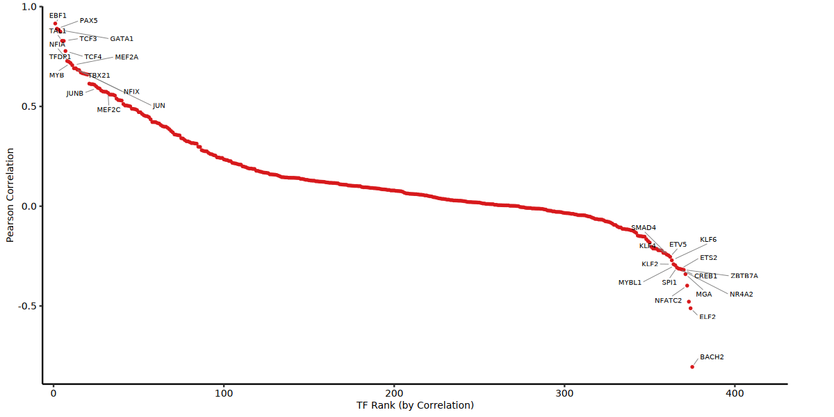

💡 Interpretation Conclusion The core TFs at both ends of the scatter plot (upper-left and lower-right corners) are the dominant regulatory hubs combining both epigenetic accessibility and gene expression characteristics. In particular, TFs in the strong positive correlation region provide extremely strong evidence that the rise in their gene expression genuinely drives the opening of the chromatin landscape at downstream target sites — these are recommended as the primary targets for subsequent in-depth analysis.

4.5 Differential TF Activity Analysis Across Cell Populations / Groups

After completing the genome-wide Motif activity computation, we similarly use the wilcoxauc function from the presto package to perform a rapid Wilcoxon rank-sum test on the scoring matrix of the chromvar Assay, identifying transcription factors (TFs) that are abnormally active in specific cell populations or states.

Consistent with the logic of differential gene expression analysis, the analysis here is also divided into two modes:

Single-Cluster TF Marker Identification Mode (Cluster vs All)
- Trigger Condition: When the group_comparison parameter is empty ("").
- Analysis Logic: The program computes the TF activity difference for each cell cluster relative to all other cells. After filtering for significantly up-/down-regulated transcription factors (p_val_adj < 0.05 and absolute logFC > logFC threshold), the results are saved as the master table All_Clusters_TF_Markers.xls.
- Visualization: To intuitively display the specific regulatory network of cell clusters, the program extracts the Top 10 core TFs for each cluster, smooths the single-cell data via Pseudobulk processing, and plots a global TF activity Z-score heatmap covering all clusters (All_Clusters_TF_Activity_Heatmap.pdf).
Intra-Cell-Type Group Comparison Mode (Case vs Control)
- Trigger Condition: When the group_comparison parameter is not empty.
- Analysis Logic: The program iterates through each cell type (e.g., B cells), comparing TF activity differences between the experimental group (case_group) and control group (control_group) within the same cell type. Filtered significant results are saved separately by cell cluster (e.g., c_Bcells_TF_Markers.xls).
- Visualization: For this mode, the program automatically generates a corresponding Volcano Plot for each cell cluster. The volcano plot highlights significantly changed (Up/Down) transcription factors in different colors, and intelligently labels the real names of the top 15 most dramatically changed up- and down-regulated TFs by logFC on the plot (e.g., c_Bcells_Case_vs_Control_TF_Activity_Volcano.pdf), helping researchers quickly pinpoint the key regulators driving disease or state changes.

if (group_comparison == "") {
    tf_markers <- wilcoxauc(
        obj,
        group_by = clusters_col,
        assay = "data",
        seurat_assay = "chromvar"
    )
    colnames(tf_markers)[2] <- "cluster"
    tf_markers$gene <- tf_markers$feature
    tf_markers$p_val_adj <- tf_markers$padj
    tf_markers$avg_log2FC <- tf_markers$logFC

    if (nrow(tf_markers) > 0) {
        
        # 1. 过滤显著差异数据（根据 logFC 绝对值 和 padj）
        sig_tf <- tf_markers[tf_markers$p_val_adj < 0.05 & abs(tf_markers$logFC) > logFC, , drop = FALSE]
        
        # 2. 覆盖保存过滤后的结果
        write.table(sig_tf, paste0(output, "/DIFF/02_motif/All_Clusters_TF_Markers.xls"),
                    quote = FALSE, row.names = FALSE, col.names = TRUE, sep = "\t")
        
        # 3. 恢复使用热图绘制 (细胞群间)
        top_tfs_df <- sig_tf %>% group_by(cluster) %>% top_n(n = 10, wt = avg_log2FC)
        top_tfs <- unique(top_tfs_df$gene)

        if (length(top_tfs) > 0) {
            cell_order <- order(factor(obj@meta.data[[clusters_col]], levels = cluster))
            cells_use <- rownames(obj@meta.data)[cell_order]

            mat <- GetAssayData(obj, assay = "chromvar", slot = "data")[top_tfs, cells_use, drop = FALSE]
            mat <- as.matrix(mat)

            cluster_vec <- as.character(obj@meta.data[cells_use, clusters_col, drop = TRUE])
            pb <- make_pseudobulk(mat, cluster_vec, pb_size = pseudobulk_size)
            mat_pb <- pb$mat

            mat_scaled <- t(scale(t(mat_pb)))
            mat_scaled[is.na(mat_scaled)] <- 0
            mat_scaled[mat_scaled > 2] <- 2
            mat_scaled[mat_scaled < -2] <- -2
            motif_names <- tryCatch({
                motif_obj <- obj@assays$ATAC@motifs
                motif_info <- motif_obj@motif.names
                sapply(rownames(mat_scaled), function(x) {
                    if (x %in% names(motif_info)) return(motif_info[[x]])
                    x
                })
            }, error = function(e) rownames(mat_scaled))
            rownames(mat_scaled) <- make.unique(as.character(motif_names))

            col_df <- data.frame(Cluster = pb$group, row.names = colnames(mat_scaled), stringsAsFactors = FALSE)
            col_anno <- HeatmapAnnotation(df = col_df, show_annotation_name = FALSE)

            ht_tf <- Heatmap(
                mat_scaled,
                cluster_rows = TRUE,
                cluster_columns = FALSE,
                show_row_names = TRUE,
                row_names_gp = gpar(fontsize = 8),
                show_column_names = FALSE,
                show_row_dend = FALSE,
                top_annotation = col_anno,
                name = "TF_Activity_Z",
                use_raster = TRUE
            )

            pdf(paste0(output, "/DIFF/02_motif/All_Clusters_TF_Activity_Heatmap.pdf"),
                width = 12, height = max(6, nrow(mat_scaled) * 0.2))
            draw(ht_tf)
            dev.off()
        }
    }
} else {
    obj_group <- obj
    Idents(obj_group) <- group_comparison

    for (i in unique(obj_group@meta.data[[clusters_col]])) {
        cells_in_cluster <- rownames(obj_group@meta.data)[obj_group@meta.data[[clusters_col]] == i]
        if (length(cells_in_cluster) < 10) next

        sub_obj <- subset(obj_group, cells = cells_in_cluster)
        valid_groups <- unique(sub_obj@meta.data[[group_comparison]])
        if (!(case_group %in% valid_groups) || !(control_group %in% valid_groups)) next

        tf_markers_all <- wilcoxauc(
            sub_obj,
            group_by = group_comparison,
            assay = "data",
             seurat_assay = "chromvar",
            groups_use = c(case_group, control_group)
        )

        tf_markers_all$gene <- tf_markers_all$feature
        tf_markers_all$p_val_adj <- tf_markers_all$padj
        tf_markers_all$avg_log2FC <- tf_markers_all$logFC

        if (nrow(tf_markers_all) > 0) {
            # 1. 过滤显著差异数据 (保留两个组的数据)
            sig_tf <- tf_markers_all[tf_markers_all$p_val_adj < 0.05 & abs(tf_markers_all$logFC) > logFC, , drop = FALSE]
            # 2. 保存过滤后的数据
            write.table(sig_tf, paste0(output, "/DIFF/02_motif/c_", gsub(" ", "", i), "_TF_Markers.xls"),
                        quote = FALSE, row.names = FALSE, col.names = TRUE, sep = "\t")

            # 3. 画火山图 (火山图通常只看 case vs control 的 logFC，所以提取 case 组的数据来画)
            volcano_data <- tf_markers_all[tf_markers_all$group == case_group, , drop = FALSE]
            volcano_data$Status <- "Not Significant"
            volcano_data$Status[volcano_data$padj < 0.05 & volcano_data$logFC > logFC] <- "Up"
            volcano_data$Status[volcano_data$padj < 0.05 & volcano_data$logFC < -logFC] <- "Down"
            
            library(ggrepel)
            
            # 由于 wilcoxauc 已经限制为 case_group 的结果，这里只画一个火山图
            vd_g <- volcano_data
            
            up_genes <- vd_g[vd_g$Status == "Up", ]
            down_genes <- vd_g[vd_g$Status == "Down", ]
            
            top_up <- up_genes[order(up_genes$logFC, decreasing = TRUE), ]
            if (nrow(top_up) > 15) top_up <- top_up[1:15, ]
            
            top_down <- down_genes[order(down_genes$logFC, decreasing = FALSE), ]
            if (nrow(top_down) > 15) top_down <- top_down[1:15, ]
            
            label_data <- rbind(top_up, top_down)
            
            # 将 motif_id 转换为实际名字
            label_data$label <- tryCatch({
                motif_info <- obj@assays$ATAC@motifs@motif.names
                sapply(label_data$feature, function(x) if (x %in% names(motif_info)) motif_info[[x]] else x)
            }, error = function(e) label_data$feature)
            
            title_txt <- paste0(i, "(", case_group, " vs ", control_group, ")")
            out_prefix <- paste0(output, "/DIFF/02_motif/c_", gsub(" ", "", i), "_", gsub(" ", "", case_group), "_vs_", gsub(" ", "", control_group), "_TF_Activity_Volcano")
            
            p_volcano <- ggplot(vd_g, aes(x = logFC, y = -log10(padj), color = Status)) +
                geom_point(alpha = 0.8, size = 1.5) +
                scale_color_manual(values = c("Up" = "#d73027", "Down" = "#4575b4", "Not Significant" = "#e0e0e0")) +
                geom_hline(yintercept = -log10(0.05), linetype = "dashed", color = "black", alpha = 0.5) +
                geom_vline(xintercept = c(-logFC, logFC), linetype = "dashed", color = "black", alpha = 0.5) +
                geom_text_repel(data = label_data, aes(label = label), size = 3, color = "black", 
                                max.overlaps = 50, segment.color = "grey50", segment.size = 0.5) +
                theme_bw() +
                theme(
                    panel.grid.major = element_blank(),
                    panel.grid.minor = element_blank(),
                    legend.position = "right",
                    legend.title = element_blank(),
                    plot.title = element_text(hjust = 0.5, face = "bold", size = 14)
                ) +
                labs(title = title_txt, x = "log2(Fold Change)", y = "-log10(padj)")
                
            ggplot2::ggsave(paste0(out_prefix, ".pdf"), plot = p_volcano, width = 7, height = 6)
            ggplot2::ggsave(paste0(out_prefix, ".png"), plot = p_volcano, width = 7, height = 6, dpi = 300)
        }
    }
}

options(repr.plot.width = 10, repr.plot.height = 7)
if (group_comparison == "") {
    draw(ht_tf)
    }else{
     p_volcano
    }

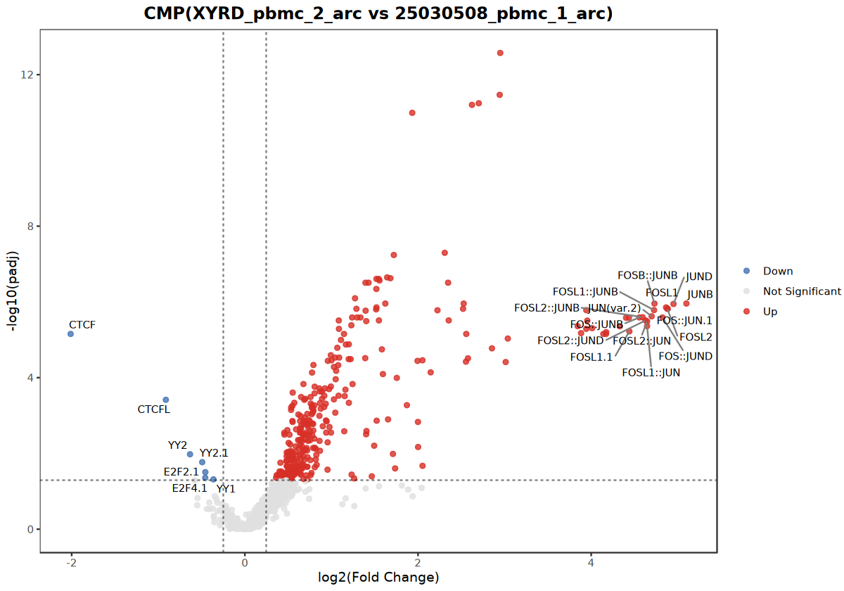
💡 Biological Significance The core purpose of this step is to distill biologically interpretable regulator clues from the massive amount of "accessibility signal changes." TFs with significantly up-regulated activity typically suggest their active participation in transcriptional activation or maintenance of cell phenotype in the target cell state; whereas down-regulated activity suggests silencing of their regulatory network. The final output list of differential TFs is the best candidate set for subsequent construction of core regulatory networks and design of mechanistic validation experiments.

data_dir <- paste0(output,"/DIFF/02_motif")

# 1. 收集并合并 TF 活性差异表格 (TF_Markers.xls)
if (group_comparison == "") {
    marker_files <- list.files(path = data_dir, pattern = "TF_Markers\\.xls$", full.names = TRUE)
} else {
    # 组间差异模式：排除掉单聚类的 All_Clusters_TF_Markers.xls 等不相关的文件，仅保留各个 cluster 分组比较生成的 marker
    marker_files <- list.files(path = data_dir, pattern = "^c_.*_TF_Markers\\.xls$", full.names = TRUE)
}

merged_markers <- data.frame()
for (file in marker_files) {
    df <- tryCatch(read.table(file, sep="\t", header=TRUE, stringsAsFactors = FALSE), error = function(e) NULL)
    if (!is.null(df) && nrow(df) > 0) {
        if ("cluster" %in% colnames(df)) df$cluster <- as.character(df$cluster)
        
        # 组间模式下补充 cluster 名称（如果是按照 c_XXX_TF_Markers 命名的）
        if (group_comparison != "" && !("cluster" %in% colnames(df))) {
            # 尝试从文件名解析 cluster name: c_Bcells_TF_Markers.xls -> Bcells
            base_name <- basename(file)
            cl_name <- gsub("^c_", "", gsub("_TF_Markers\\.xls$", "", base_name))
            df$cluster <- cl_name
        }
        
        # 确保当前已有的 merged_markers 也不是空的，或者这是第一次合并
        if (nrow(merged_markers) == 0) {
            merged_markers <- df
        } else {
            merged_markers <- bind_rows(merged_markers, df)
        }
    }
}

if (group_comparison != "" && nrow(merged_markers) > 0) {
    # 如果是组间差异模式，将其保存到 all_TF_Markers.xls 供交互展示和下载
    write.table(merged_markers[which(merged_markers$logFC > 0),],
                file = paste0(output, '/DIFF/02_motif/all_TF_Markers.xls'),
                quote = F, row.names = F, col.names = T, sep = '\t')
}

head(merged_markers)

A data.frame: 6 × 14
	feature	group	avgExpr	logFC	statistic	auc	pval	padj	pct_in	pct_out	gene	p_val_adj	avg_log2FC	cluster
	<chr>	<chr>	<dbl>	<dbl>	<dbl>	<dbl>	<dbl>	<dbl>	<int>	<int>	<chr>	<dbl>	<dbl>	<chr>
1	MA0002.1	25030508_pbmc_1_arc	-1.40086958	-0.4710262	150256	0.3696662	2.112365e-09	1.645207e-08	100	100	MA0002.1	1.645207e-08	-0.4710262	Bcells
2	MA0003.1	25030508_pbmc_1_arc	0.33990583	-0.4448016	155355	0.3822110	6.215919e-08	3.596353e-07	100	100	MA0003.1	3.596353e-07	-0.4448016	Bcells
3	MA0048.1	25030508_pbmc_1_arc	2.92851842	-0.9484831	160852	0.3957349	1.659225e-06	6.822194e-06	100	100	MA0048.1	6.822194e-06	-0.9484831	Bcells
4	MA0050.1	25030508_pbmc_1_arc	0.01236445	-1.1000062	107759	0.2651133	3.704878e-27	1.364069e-25	100	100	MA0050.1	1.364069e-25	-1.1000062	Bcells
5	MA0051.1	25030508_pbmc_1_arc	-0.73876620	-0.9485148	116735	0.2871964	1.392626e-22	4.338566e-21	100	100	MA0051.1	4.338566e-21	-0.9485148	Bcells
6	MA0052.1	25030508_pbmc_1_arc	0.82173660	-0.4136321	155320	0.3821249	6.079983e-08	3.568686e-07	100	100	MA0052.1	3.568686e-07	-0.4136321	Bcells

💡 Interpretation Guide
This table displays the differential analysis results of TF binding site accessibility computed based on chromVAR. It can be used to identify core regulators whose activity changes significantly in specific cell subpopulations or disease groups. The key metrics to focus on are padj significance and logFC fold difference.
feature: Motif ID, e.g., MA0494.1.
cluster / group: The cell cluster or corresponding group in which the TF activity has changed significantly.
auc: Area Under the Curve, used to evaluate the classification performance of this TF activity as a marker distinguishing this group of cells. Values closer to 1 or 0 indicate stronger discriminative power.
pval / padj: Raw P-value and P-value after multiple-testing correction. Typically, padj < 0.05 is used as the criterion for significant change.
logFC: Average log fold change. A positive value indicates enhanced activity and increased openness of this TF in the current target group; a negative value indicates reduced activity.
pct_in / pct_out: Proportion of cells in the target group and background group, respectively, in which this TF activity is detected.

5. Motif Enrichment Analysis

Motif enrichment analysis is a completely different concept from the preceding Motif activity analysis:

Motif activity analysis computes a genome-wide score for each single cell's overall accessibility against a specific Motif across all regions (based on background variation).
Motif enrichment analysis, on the other hand, is based on a given specific sequence set (e.g., the identified differential Peak regions) and uses statistical methods such as the hypergeometric test to identify which transcription factor Motifs appear at a frequency in these specific sequences significantly higher than in the background sequences. This is typically used to find the core transcription factors regulating specific biological processes.

5.1 Differential Peak Dataset Preparation

Before performing Motif enrichment, first use wilcoxauc to obtain the differential Peak set containing the target regions. Consistent with the preceding analysis logic, this step will also automatically switch between two modes based on the value of the group_comparison parameter:

Single-Cluster Marker Mode (group_comparison == ""): Identify characteristic differential Peaks for each cell cluster relative to all other cells.
Intra-Cell-Type Group Difference Mode (group_comparison != ""): Iterate through each cell cluster, extracting differential Peaks that change significantly between the experimental group (Case) and control group (Control), and merge all cluster results for export as all_diffPeak.xls for downstream analysis.

if (group_comparison == "") {
    da_peaks <- wilcoxauc(obj, clusters_col, assay='data', seurat_assay='ATAC')
    colnames(da_peaks)[2] <- 'cluster'
} else {
    all_da_peaks <- list()
    obj <- subset(obj, subset = !!sym(group_comparison) %in% c(case_group, control_group))
    
    for (cell_type_analyse in unique(obj@meta.data[[clusters_col]])) {
        tryCatch({
            sub_obj <- subset(obj, subset = !!sym(clusters_col) %in% cell_type_analyse)
            da_peaks <- wilcoxauc(sub_obj, 
                                        group_by = group_comparison, 
                                        assay = 'data',
                                        seurat_assay = 'ATAC',
                                        groups_use = c(case_group, control_group))
            da_peaks$cluster <- as.character(cell_type_analyse)
            all_da_peaks[[as.character(cell_type_analyse)]] <- da_peaks
        }, error = function(e) {
        message(sprintf("Error in cluster %s: %s", cell_type_analyse, e$message))
        })
    }
    da_peaks <- do.call(rbind, all_da_peaks)

    write.table(da_peaks,
               file = paste0(output, '/DIFF/all_diffPeak.xls'),
               quote = F, row.names = F, col.names = T, sep = '\t')
}
saveRDS(obj,paste0(output, '/output.rds'))
write.table(da_peaks[da_peaks$padj < pval_adj & da_peaks$logFC > logFC, ],paste0(output,'/DIFF/01_diffPeak/all_diffPeak_significant.xls'),quote=F,row.names=F,col.names=T,sep='\t')

5.2 Motif Enrichment Analysis and Visualization of Differential Peaks

After successfully identifying significantly differential Peaks across cell clusters or experimental groups, we proceed to perform Motif enrichment analysis on these specifically accessible chromatin regions. The core purpose of this step is: to trace back from the epigenetic phenomenon (accessibility) to the upstream regulatory mechanism, identifying the potential dominant transcription factors (TFs) truly driving the opening of these regions.

Motif Enrichment and Multi-Dimensional Evidence Integration: We use the FindMotifs function to detect whether binding motifs of specific transcription factors are significantly enriched in differential Peaks. To improve result confidence, the program automatically associates this enrichment result with the previously computed global TF expression–activity correlation matrix for cross-integration. Through this multi-dimensional cross-validation, we can precisely filter out those "genuine" drivers that are not only highly enriched in local differential Peaks but also show a strong positive correlation between their RNA expression level and chromatin accessibility activity at the global level (analysis results will be uniformly output to the 02_motif directory).
Intuitive Visualization of Enrichment Features: To help researchers more intuitively interpret the regulatory network, the program automatically extracts the most statistically significant key features for multi-dimensional visualization:
- Motif Heatmap Composite Plot: Display the accessibility signal distribution of differential Peaks in heatmap form, with significantly enriched core Motifs precisely marked by connecting lines on the right side.
- Sequence Logo: Intuitively display the nucleotide preference of the Top enriched Motifs.
- Single-Cell Activity Projection Plot (UMAP): Map the ChromVAR activity scores of these Top Motifs onto the UMAP dimensionality-reduction space, displaying their heterogeneous distribution across different single-cell populations.

cluster <- unique(da_peaks$cluster)
# 通用排序函数
sort_clusters <- function(x) {
  if(all(!is.na(suppressWarnings(as.numeric(x))))) {
    return(x[order(as.numeric(x))])
  } else {
    nums <- suppressWarnings(as.numeric(gsub("[^0-9]", "", x)))
    if(all(!is.na(nums))) {
      return(x[order(nums)])
    } else {
      return(sort(x))
    }
  }
}
cluster <- sort_clusters(cluster)

for (i in cluster) { 
    tryCatch({ 
        DefaultAssay(obj) <- "ATAC" 
        data <- da_peaks[da_peaks$cluster == i, ] 
        # 使用正则表达式检查 feature 列的格式 染色体-起始-终止 
        valid_rows <- grepl("^([^-]+)-(\\d+)-(\\d+)$", data$feature) 
        if (sum(!valid_rows) > 0) { 
            message(sprintf("Cluster %s: Removed %d malformed feature rows.", i, sum(!valid_rows))) 
            data <- data[valid_rows, ] 
        } 
        
        # Determine the groups to iterate over based on group_comparison 
        if (group_comparison == "") { 
            # Standard single cluster comparison 
            analysis_groups <- c("cluster_marker") 
        } else { 
            # Two group comparison: case and control 
            analysis_groups <- c(case_group, control_group) 
        } 
        
        for (grp in analysis_groups) { 
            print(paste0("正在分析：Cluster ", i, " - Group ", grp)) 
            tryCatch({ 
                if (grp == "cluster_marker") { 
                    # For single cluster, we use padj < pval_adj and logFC > logFC 
                    data.sig <- data[data$padj < pval_adj & data$logFC > logFC, ] 
                    prefix <- paste0('c_', gsub(" ", "", i)) 
                } else { 
                    # For group comparison, filter by group and thresholds 
                    data.sig <- data[data$group == grp & data$padj < pval_adj & data$logFC > logFC, ] 
                    prefix <- paste0('c_', gsub(" ", "", i), '_', gsub(" ", "", grp)) 
                } 
                
                if (nrow(data.sig) == 0) { 
                    message(sprintf("No significant peaks found for %s", prefix)) 
                    next 
                } 
                
                peaks <- data.sig$feature 
                
                # --- FindMotifs 分析核心开始 ---
                enriched.motifs <- FindMotifs(object = obj, features = peaks) 
                enriched.motifs$cluster <- as.character(i) 
                if (grp != "cluster_marker") enriched.motifs$group <- as.character(grp) 
                
                if (!is.na(expr_assay) && nrow(enriched.motifs) > 0 && "motif.name" %in% colnames(enriched.motifs)) { 
                    if (grp == "cluster_marker") { 
                        cells_expr <- rownames(obj@meta.data)[obj@meta.data[[clusters_col]] == i] 
                    } else { 
                        cells_expr <- rownames(obj@meta.data)[obj@meta.data[[clusters_col]] == i & obj@meta.data[[group_comparison]] == grp] 
                    } 
                    if (length(cells_expr) > 0) { 
                        expr_mat <- GetAssayData(obj, assay = expr_assay, slot = "data")[, cells_expr, drop = FALSE] 
                        expr_pct <- rowMeans(expr_mat > 0) 
                        # 修正：将原代码的 spe 改为环境中已有的 species 变量
                        expressed_tfs <- normalize_tf_names(rownames(expr_mat)[expr_pct >= 0.01], species_name = species) 
                        motif_tf_list <- lapply(enriched.motifs$motif.name, extract_motif_tfs, species_name = species) 
                        enriched.motifs$motif_tf <- vapply(motif_tf_list, function(x) paste(x, collapse = "::"), character(1)) 
                        enriched.motifs$tf_in_rna <- vapply(motif_tf_list, function(x) any(x %in% expressed_tfs), logical(1)) 
                        enriched.motifs <- enriched.motifs[enriched.motifs$tf_in_rna, , drop = FALSE] 
                    } else { 
                        enriched.motifs <- enriched.motifs[0, , drop = FALSE] 
                    } 
                } 
                
                enriched.motifs <- enriched.motifs[which(enriched.motifs$p.adjust < 0.05 & enriched.motifs$fold.enrichment > 1), , drop = FALSE]                                       
                
                # 修正：将 03_motif 改为 02_motif，解决与后续合并代码的目录冲突问题
                write.table(enriched.motifs, paste0(output,'/DIFF/02_motif/', prefix, '_diffPeak_motifs.xls'), quote=F, row.names=F, col.names=T, sep='\t') 
                
                if (!is.na(expr_assay) && nrow(enriched.motifs) > 0) { 
                    if (!is.null(global_tf_corr)) { 
                        tf_corr_subset <- global_tf_corr[global_tf_corr$motif_id %in% rownames(enriched.motifs), , drop = FALSE] 
                        if (nrow(tf_corr_subset) > 0) { 
                            motif_meta <- enriched.motifs 
                            motif_meta$motif_id <- rownames(motif_meta) 
                            keep_cols <- c("motif_id", "fold.enrichment", "cluster", "group", "p.adjust") 
                            keep_cols <- keep_cols[keep_cols %in% colnames(motif_meta)] 
                            motif_meta <- motif_meta[, keep_cols, drop = FALSE] 
                            tf_corr_subset <- dplyr::left_join(tf_corr_subset, motif_meta, by = "motif_id") 
                            
                            if (!("fold.enrichment" %in% colnames(tf_corr_subset))) tf_corr_subset$fold.enrichment <- NA_real_ 
                            if (!("cluster" %in% colnames(tf_corr_subset))) tf_corr_subset$cluster <- as.character(i) 
                            if (!("group" %in% colnames(tf_corr_subset))) tf_corr_subset$group <- if (grp == "cluster_marker") "" else as.character(grp) 
                            if (!("p.adjust" %in% colnames(tf_corr_subset))) tf_corr_subset$p.adjust <- NA_real_ 
                            
                            tf_corr_subset$high_cor <- tf_corr_subset$pearson_cor > cor 
                            
                            tf_corr_subset <- tf_corr_subset[, c( 
                                "motif_id", "motif_name", "TF", "fold.enrichment", "p.adjust", "cluster", "group", 
                                "expr_pct", "expr_mean", "activity_mean", "pearson_cor", "p_value", "high_cor" 
                            ), drop = FALSE] 
                            
                            # 修正：将 03_motif 改为 02_motif
                            write.table(tf_corr_subset, paste0(output, "/DIFF/02_motif/", prefix, "_TF_ActExpr_Correlation.xls"), quote = FALSE, row.names = FALSE, col.names = TRUE, sep = "\t") 
                        } 
                    } 
                } 
                
            }, error = function(e) { 
                message(sprintf("Error in cluster %s, group %s: %s", i, grp, e$message)) 
            }) 
        } 
        print(paste0("Cluster ", i, " 分析完成")) 
    }, error = function(e) { 
        message(sprintf("Error in cluster %s: %s", i, e$message)) 
    }) 
}

tryCatch({
    ensure_color_map <- function(values, color_map) {
        values <- unique(as.character(values))
        values <- values[!is.na(values)]
        if (!all(values %in% names(color_map))) {
            miss <- setdiff(values, names(color_map))
            if (length(miss) > 0) {
                extra_cols <- setNames(scales::hue_pal()(length(miss)), miss)
                color_map <- c(color_map, extra_cols)
            }
        }
        color_map
    }



    build_mark <- function(group_vec, label_map) { 
        lv <- unique(as.character(group_vec)) 
        lv <- lv[!is.na(lv)] 
        at <- unname(vapply(lv, function(g) { 
            idx <- which(as.character(group_vec) == g) 
            idx[(length(idx) + 1) %/% 2] 
        }, integer(1))) 
        labels <- unname(label_map[lv]) 
        
        # 去除尾部可能的多余空格
        labels <- gsub("\\s+$", "", labels) 
        
        # 新增：找出不是空字符串的索引，只保留有文本的标记
        valid_idx <- which(labels != "")
        
        # 只返回有效的 at, labels 和 levels
        list(at = at[valid_idx], labels = labels[valid_idx], levels = lv[valid_idx]) 
    } 


    


    if (group_comparison == "") {
        all_top_peaks <- c()
        peak_cluster_anno <- c()
        motif_text_anno <- c()

        for (i in cluster) {
            data.sig <- da_peaks[da_peaks$cluster == i & da_peaks$padj < pval_adj & da_peaks$logFC > logFC, ]
            if (nrow(data.sig) > 0) {
                data.sig <- data.sig[order(data.sig$logFC, decreasing = TRUE), ]
                top_n <- min(nrow(data.sig), 500)
                sel_peaks <- data.sig$feature[1:top_n]

                all_top_peaks <- c(all_top_peaks, sel_peaks)
                peak_cluster_anno <- c(peak_cluster_anno, rep(i, top_n))

                prefix <- paste0("c_", gsub(" ", "", i))
                motif_file <- paste0(output, "/DIFF/02_motif/", prefix, "_diffPeak_motifs.xls")
                motif_text <- get_group_motif_text(motif_file, fe_cut = fe_cut, top_n = 6, n_col = 3, n_row = 2)
                motif_text_anno <- c(motif_text_anno, motif_text)
            }
        }

        if (length(all_top_peaks) > 0) {
            active_clusters <- unique(peak_cluster_anno)
            names(motif_text_anno) <- active_clusters

            cell_order <- order(factor(obj@meta.data[[clusters_col]], levels = cluster))
            cells_use <- rownames(obj@meta.data)[cell_order]

            DefaultAssay(obj) <- "ATAC"
            mat <- GetAssayData(obj, assay = "ATAC", slot = "data")[all_top_peaks, cells_use, drop = FALSE]
            mat <- as.matrix(mat)

            cluster_vec <- as.character(obj@meta.data[cells_use, clusters_col, drop = TRUE])
            pb <- make_pseudobulk(mat = mat, groups = cluster_vec, pb_size = pseudobulk_size)
            mat <- pb$mat
            col_df <- data.frame(Cluster = pb$group, row.names = colnames(mat), stringsAsFactors = FALSE)

            mat_scaled <- t(scale(t(mat)))
            mat_scaled[is.na(mat_scaled)] <- 0
            mat_scaled[mat_scaled > 2] <- 2
            mat_scaled[mat_scaled < -2] <- -2

            cols_use <- ensure_color_map(col_df$Cluster, group_colors)

            col_anno <- HeatmapAnnotation(
                df = col_df,
                col = list(Cluster = cols_use),
                show_annotation_name = FALSE
            )

            mark <- build_mark(peak_cluster_anno, motif_text_anno)

                    right_anno <- rowAnnotation(
                        Motifs = anno_mark(
                            at = mark$at,                 # 仍然是你算好的目标行中心
                            labels = mark$labels,         # 文本可长，可多行
                            which = "row",
                            side = "right",
                            labels_gp = gpar(fontsize = 8, lineheight = 1.2,fontface = "bold",col = "black"),
                            lines_gp = gpar(col = "black", lty = 1),   # 线样式
                            link_width = unit(4, "mm"),  
                           # just = c("right","top"),# 横向“引出段”，越大越明显折线感
                            padding = unit(0.1, "mm"),                 # 标签间距
                            extend = unit(c(1, 1), "mm")               # 把标签整体往右推，制造更多折线空
                        )#,
                        #width = unit(5, "cm")
                    )

            col_fun <- circlize::colorRamp2(
                c(-2, -1, 0, 1, 2),
                c("#2c7bb6", "#abd9e9", "#f7f7f7", "#fdae61", "#d7191c")
            )

            ht <- Heatmap(
                mat_scaled,
                col = col_fun,
                cluster_rows = FALSE,
                cluster_columns = FALSE,
                show_row_names = FALSE,
                show_column_names = FALSE,
                show_row_dend = FALSE,
                row_title_rot = 0,
                top_annotation = col_anno,
                right_annotation = right_anno,
                name = "Accessibility",
                use_raster = TRUE
            )

            pdf(paste0(output, "/DIFF/01_diffPeak/All_Clusters_DiffPeak_Heatmap.pdf"), width = 12, height = 10)
            draw(ht,padding = unit(c(10, 6, 6, 10), "mm"))
            dev.off()
        }
    } else {
        for (i in cluster) {
            data.sig <- da_peaks[da_peaks$cluster == i & da_peaks$padj < pval_adj & da_peaks$logFC > logFC, ]
            if (nrow(data.sig) > 0) {
                sel_peaks <- c()
                peak_group_anno <- c()
                motif_text_map <- setNames(rep("", 2), c(case_group, control_group))

                for (grp in c(case_group, control_group)) {
                    data.grp <- data.sig[data.sig$group == grp, ]
                    if (nrow(data.grp) > 0) {
                        data.grp <- data.grp[order(data.grp$logFC, decreasing = TRUE), ]
                        top_n <- min(nrow(data.grp), 500)
                        grp_peaks <- data.grp$feature[1:top_n]

                        sel_peaks <- c(sel_peaks, grp_peaks)
                        peak_group_anno <- c(peak_group_anno, rep(grp, top_n))

                        prefix <- paste0("c_", gsub(" ", "", i), "_", gsub(" ", "", grp))
                        motif_file <- paste0(output, "/DIFF/02_motif/", prefix, "_diffPeak_motifs.xls")
                        motif_text_map[grp] <- get_group_motif_text(motif_file, fe_cut = fe_cut, top_n = 20)
                    }
                }

                cells_in_cluster <- rownames(obj@meta.data)[obj@meta.data[[clusters_col]] == i]
                sub_meta <- obj@meta.data[cells_in_cluster, , drop = FALSE]
                cell_order <- order(factor(sub_meta[[group_comparison]], levels = c(case_group, control_group)))
                cells_use <- cells_in_cluster[cell_order]

                if (length(cells_use) > 0 && length(sel_peaks) > 0) {
                    active_groups <- c(case_group, control_group)[c(case_group, control_group) %in% unique(peak_group_anno)]
                    motif_text_anno <- motif_text_map[active_groups]

                    DefaultAssay(obj) <- "ATAC"
                    mat <- GetAssayData(obj, assay = "ATAC", slot = "data")[sel_peaks, cells_use, drop = FALSE]
                    mat <- as.matrix(mat)

                    group_vec <- as.character(sub_meta[cells_use, group_comparison, drop = TRUE])
                    pb <- make_pseudobulk(mat = mat, groups = group_vec, pb_size = pseudobulk_size)
                    mat <- pb$mat
                    col_df <- data.frame(Group = pb$group, row.names = colnames(mat), stringsAsFactors = FALSE)

                    mat_scaled <- t(scale(t(mat)))
                    mat_scaled[is.na(mat_scaled)] <- 0
                    mat_scaled[mat_scaled > 2] <- 2
                    mat_scaled[mat_scaled < -2] <- -2

                    cols_use <- ensure_color_map(col_df$Group, group_colors)

                    col_anno <- HeatmapAnnotation(
                        df = col_df,
                        col = list(Group = cols_use),
                        show_annotation_name = FALSE
                    )

                    mark <- build_mark(peak_group_anno, motif_text_anno)
                    right_anno <- rowAnnotation(
                        Motifs = anno_mark(
                            at = mark$at,                 # 仍然是你算好的目标行中心
                            labels = mark$labels,         # 文本可长，可多行
                            which = "row",
                            side = "right",
                            labels_gp = gpar(fontsize = 8, lineheight = 1.2,fontface = "bold",col = "black"),
                            lines_gp = gpar(col = "black", lty = 2),   # 线样式
                            link_width = unit(4, "mm"),  
                           # just = c("right","top"),# 横向“引出段”，越大越明显折线感
                            padding = unit(0.5, "mm"),                 # 标签间距
                            extend = unit(c(1, 5), "mm")               # 把标签整体往右推，制造更多折线空
                        ),
                        width = unit(5, "cm")
                    )

                    col_fun <- circlize::colorRamp2(
                        c(-2, -1, 0, 1, 2),
                        c("#2c7bb6", "#abd9e9", "#f7f7f7", "#fdae61", "#d7191c")
                    )

                    ht <- Heatmap(
                        mat_scaled,
                        col = col_fun,
                        cluster_rows = FALSE,
                        cluster_columns = FALSE,
                        show_row_names = FALSE,
                        show_column_names = FALSE,
                        show_row_dend = FALSE,
                        row_title_rot = 0,
                        top_annotation = col_anno,
                        right_annotation = right_anno,
                        name = "Accessibility",
                        column_title = paste0("Cluster: ", i),
                        use_raster = TRUE
                    )

                    pdf(paste0(output, "/DIFF/01_diffPeak/c_", gsub(" ", "", i), "_Group_DiffPeak_Heatmap.pdf"), width = 8, height = 7)
                    draw(ht,padding = unit(c(10, 6, 6, 10), "mm"))
                    dev.off()
                }
            }
        }
    }
}, error = function(e) {
    message("Error in drawing heatmaps: ", e$message)
})

options(repr.plot.width = 15, repr.plot.height = 7)
draw(ht,padding = unit(c(10, 6, 6, 10), "mm"))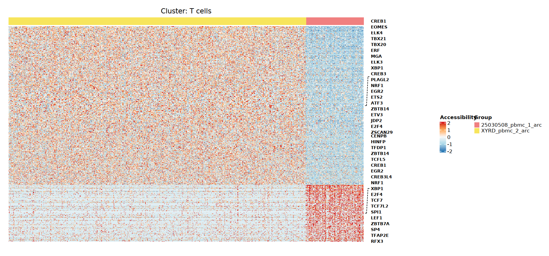

💡 Note
The example heatmap here displays the chromatin accessibility distribution of differential Peaks between T cell subgroups, with significantly enriched core transcription factor Motifs marked by connecting lines on the right side of these regions.
Heatmap Color (Z-score): Colors from blue to red (or according to the set palette) reflect the relative accessibility of specific chromatin regions across cell clusters or sample groups. Deeper red indicates higher openness of that region; deeper blue indicates that region tends toward closure.
X-axis (Columns): Represents cell clusters (or comparison groups) smoothed via Pseudobulk processing. The top color bar (Column Annotation) is used to distinguish different cell types or samples.
Y-axis (Rows): Represents identified significant differential Peaks (specific accessible regions). Rows do not display specific names but are clustered and ordered by their belonging cell cluster or group.
Right-Side Labels (Motifs): Extracts the names of Top Motifs with the highest fold enrichment in the corresponding differential Peak set. By inspecting these labels, one can quickly and intuitively link specific accessible regions to their potential upstream driver transcription factors.

5.3 Motif Enrichment Result Summarization

In the preceding loop analysis, the program has already generated separate Motif enrichment result files for each cell cluster (or comparison group) (e.g., c_Bcells_diffPeak_motifs.xls). To facilitate subsequent global preview, statistics, and downstream pathway analysis, we need to merge these scattered files into a single complete master table.

The core logic of this code is as follows:

Automatic File Retrieval: Scan the 02_motif result directory for all separately generated enrichment result tables via the regular expression motifs\.xls$.
Safe Reading and Merging: Use a loop to sequentially read these files. During reading, the program has a built-in safety mechanism that automatically skips empty files with size 0 or data frames with 0 rows (this typically occurs when certain cell clusters have no significantly enriched Motifs identified).
Data Type Unification: Before performing rbind merging, forcibly convert all columns to character type (character), avoiding merging failures caused by inconsistent type inference in certain columns across individual files (e.g., cluster with purely numeric names).
Output Summarized Results: Finally generate a merged_data master table containing significantly enriched Motif information across all groups and all cell clusters, facilitating global search and comparison for researchers.

# 最简单的合并版本
data_dir <- paste0(output, "/DIFF/02_motif")
xls_files <- list.files(path = data_dir, 
                       pattern = "motifs\\.xls$", 
                       full.names = TRUE)

merged_data <- data.frame()

for (file in xls_files) {
    # 跳过空文件
    if (file.size(file) == 0) next
    
    # 读取数据
    df <- read.table(file, sep = "\t", header = TRUE, 
                    stringsAsFactors = FALSE)
    
    # 跳过空数据框
    if (nrow(df) == 0) next
    
    # 强制所有列为字符型
    df[] <- lapply(df, as.character)
    
    # 合并
    merged_data <- rbind(merged_data, df)
}

# 处理cluster列
if (nrow(merged_data) > 0 && "cluster" %in% colnames(merged_data)) {
    merged_data$cluster <- as.character(merged_data$cluster)
}

cat("合并了", nrow(merged_data), "行数据\n")

head(merged_data)

output

合并了 1283 行数据

A data.frame: 6 × 13
	motif	observed	background	percent.observed	percent.background	fold.enrichment	pvalue	motif.name	p.adjust	cluster	group	motif_tf	tf_in_rna
	<chr>	<chr>	<chr>	<chr>	<chr>	<chr>	<chr>	<chr>	<chr>	<chr>	<chr>	<chr>	<chr>
1	MA1548.1	13	5506	41.9354838709677	13.765	3.04652988528643	0.000113293420229509	PLAGL2	0.0229419175964756	B cells	25030508_pbmc_1_arc	PLAGL2	TRUE
2	MA1648.1	454	7960	36.6720516962843	19.9	1.84281666815499	3.60213197709286e-44	TCF12(var.2)	3.24191877938358e-42	B cells	XYRD_pbmc_2_arc	TCF12	TRUE
3	MA1558.1	471	8486	38.0452342487884	21.215	1.79331766433129	5.39243273131294e-43	SNAI1	3.9707913748759e-41	B cells	XYRD_pbmc_2_arc	SNAI1	TRUE
4	MA0830.1	438	7946	35.3796445880452	19.865	1.78100400644577	1.99335037013957e-38	TCF4	1.15329557129504e-36	B cells	XYRD_pbmc_2_arc	TCF4	TRUE
5	MA0107.1	297	4474	23.9903069466882	11.185	2.14486427775487	2.60148879508546e-38	RELA	1.31700370251201e-36	B cells	XYRD_pbmc_2_arc	RELA	TRUE
6	MA0105.1	277	4121	22.3747980613893	10.3025	2.17178335951365	2.07812263197394e-36	NFKB1	8.41639665949446e-35	B cells	XYRD_pbmc_2_arc	NFKB1	TRUE

💡 Note
This table displays "which Motifs are enriched in differentially accessible Peaks," providing statistical significance, enrichment fold, and RNA expression support information. Each row corresponds to a Motif candidate; the key metrics to focus on are p.adjust, fold.enrichment, and tf_in_rna.
motif: Motif ID, e.g., MA0494.1, typically from JASPAR, uniquely identifying the sequence pattern.
motif.name: Readable TF/Motif name, e.g., Bach1::Mafk, RUNX1; dual-TF names usually indicate composite or family-related patterns.
observed: Number of Peaks in the target differential Peak set that match this Motif.
background: Number of Peaks in the background Peak set that match this Motif.
percent.observed / percent.background: Percentage of Motif matches in the target set and background set, used to intuitively assess enrichment direction.
fold.enrichment: Enrichment fold, i.e., target proportion / background proportion; >1 indicates enrichment, with larger values indicating stronger enrichment.
pvalue: Raw significance P-value.
p.adjust: P-value after multiple-testing correction; typically used as the primary criterion for significance judgment, with p.adjust < 0.05 considered significantly enriched.
cluster / group: Cell cluster and comparison group.
motif_tf: Normalized TF name, used for matching with RNA gene names.
tf_in_rna: Whether there is RNA expression support; TRUE indicates that the proportion of cells expressing the TF corresponding to this Motif in the target cell cluster reaches the 10% threshold.

5.4 TF Activity vs DiffPeak Enriched Motif Overlap Analysis (Venn Diagram)

To determine whether a TF has genuinely played a key regulatory role in the current cell state, single-dimension analysis is often insufficient. This step uses a Venn diagram to cross-validate evidence from two independent analytical dimensions:

Dimension 1: Sequence Enrichment Evidence — answers "Is this TF's binding sequence abnormally dense in differentially accessible chromatin regions?"
Dimension 2: Genome-Wide Activity Change Evidence — answers "At the genome-wide level, has the overall accessibility of this TF's potential binding sites changed significantly?"

By comparing these two sets, we can filter the large number of candidate TFs. The intersection in the middle of the Venn diagram represents TFs that are both recruited in local differential regions and exhibit active status at the genome-wide level.

💡 Interpretation Conclusion Motifs located in the intersection region of the Venn diagram have the highest level of confidence — they are the core dominant TFs. When designing subsequent molecular biological mechanistic validation (e.g., ChIP-seq, CRISPR knockout) or constructing upstream core regulatory networks, prioritize these intersecting TFs as the first-priority candidate targets.

library(VennDiagram) 
library(grid) 
 
motif_dir <- file.path(output, "DIFF", "02_motif") 
venn_dir  <- file.path(motif_dir, "motif_overlap_venn") 
dir.create(venn_dir, recursive = TRUE, showWarnings = FALSE) 
 
all_stat <- list() 
k <- 0 
 
if (group_comparison == "") { 
  tf_file <- file.path(motif_dir, "All_Clusters_TF_Markers.xls")
  
  if (!file.exists(tf_file)) {
    warning(paste("跳过: 找不到文件", tf_file))
  } else {
    tf_df <- read.delim( 
      tf_file, 
      sep = "\t", check.names = FALSE, stringsAsFactors = FALSE 
    ) 
    
    for (cl in as.character(cluster)) { 
      cl_s <- gsub(" ", "", cl) 
      motif_file <- file.path(motif_dir, paste0("c_", cl_s, "_diffPeak_motifs.xls"))
      
      if (!file.exists(motif_file)) {
        warning(paste("跳过: 找不到文件", motif_file))
        next
      }
      
      motif_df <- read.delim( 
        motif_file, 
        sep = "\t", check.names = FALSE, stringsAsFactors = FALSE 
      ) 
      
      tf_col <- intersect(c("gene", "feature", "motif", "motif_id", "motif.name", "name"), colnames(tf_df))[1] 
      motif_col <- intersect(c("motif", "motif_id", "motif.name", "feature", "gene", "name"), colnames(motif_df))[1] 
      
      tf_raw <- trimws(as.character(tf_df[tf_df$cluster == cl, tf_col, drop = TRUE])) 
      motif_raw <- trimws(as.character(motif_df[[motif_col]])) 
      
      tf_set <- unique(tf_raw[nzchar(tf_raw)]) 
      motif_set <- unique(motif_raw[nzchar(motif_raw)]) 
      
      inter <- intersect(tf_set, motif_set) 
      jac <- if (length(union(tf_set, motif_set)) == 0) NA_real_ else length(inter) / length(union(tf_set, motif_set)) 
      
      out_prefix <- file.path(venn_dir, paste0("c_", cl_s, "_TFvsDiffPeak_motif_overlap_venn")) 
      title_txt <- paste0("Cluster: ", cl) 
      
      write.table( 
        data.frame( 
          label = title_txt, 
          TF_marker_n = length(tf_set), 
          DiffPeak_motif_n = length(motif_set), 
          overlap_n = length(inter), 
          jaccard = jac, 
          stringsAsFactors = FALSE 
        ), 
        paste0(out_prefix, "_summary.xls"), 
        sep = "\t", quote = FALSE, row.names = FALSE 
      ) 
      
      write.table( 
        data.frame(Motif = sort(inter), stringsAsFactors = FALSE), 
        paste0(out_prefix, "_overlap_motifs.xls"), 
        sep = "\t", quote = FALSE, row.names = FALSE 
      ) 
      
      out_file <- paste0(out_prefix, ".pdf") 
      grDevices::pdf(out_file, width = 6, height = 6, onefile = TRUE) 
      grid::grid.newpage() 
      if (length(tf_set) == 0 && length(motif_set) == 0) { 
        grid::grid.text(paste0(title_txt, "\n无可用motif"), x = 0.5, y = 0.5) 
      } else { 
        venn_grob <- VennDiagram::draw.pairwise.venn( 
          area1 = length(tf_set), 
          area2 = length(motif_set), 
          cross.area = length(inter), 
          category = c("Activity markers", "Enriched motifs"), 
          fill = c("#60a5fa", "#f59e0b"), 
          inverted = length(tf_set) < length(motif_set),
          alpha = c(0.5, 0.5), 
          cex = 1.2, 
          cat.cex = 1.0, 
          scaled = FALSE, 
          ind = FALSE,
          cat.pos = c(-30, 30),
          cat.dist = c(-0.05, -0.05)
        ) 
        grid::grid.draw(venn_grob) 
        grid::grid.text(title_txt, x = 0.5, y = 0.96, gp = grid::gpar(fontface = "bold")) 
      } 
      grDevices::dev.off() 
      
      k <- k + 1 
      all_stat[[k]] <- data.frame(mode = "cluster", cluster = cl, group = "", stringsAsFactors = FALSE) 
    } 
  }
} else { 
  for (cl in as.character(cluster)) { 
    cl_s <- gsub(" ", "", cl) 
    tf_file <- file.path(motif_dir, paste0("c_", cl_s, "_TF_Markers.xls"))
    
    if (!file.exists(tf_file)) {
      warning(paste("跳过: 找不到文件", tf_file))
      next
    }
    
    tf_df <- read.delim( 
      tf_file, 
      sep = "\t", check.names = FALSE, stringsAsFactors = FALSE 
    ) 
    
    for (g in as.character(c(case_group, control_group))) { 
      g_s <- gsub(" ", "", g) 
      motif_file <- file.path(motif_dir, paste0("c_", cl_s, "_", g_s, "_diffPeak_motifs.xls"))
      
      if (!file.exists(motif_file)) {
        warning(paste("跳过: 找不到文件", motif_file))
        next
      }
      
      motif_df <- read.delim( 
        motif_file, 
        sep = "\t", check.names = FALSE, stringsAsFactors = FALSE 
      ) 
      
      tf_col <- intersect(c("gene", "feature", "motif", "motif_id", "motif.name", "name"), colnames(tf_df))[1] 
      motif_col <- intersect(c("motif", "motif_id", "motif.name", "feature", "gene", "name"), colnames(motif_df))[1] 
      
      tf_raw <- trimws(as.character(tf_df[tf_df$group == g, tf_col, drop = TRUE])) 
      motif_raw <- trimws(as.character(motif_df[[motif_col]])) 
      
      tf_set <- unique(tf_raw[nzchar(tf_raw)]) 
      motif_set <- unique(motif_raw[nzchar(motif_raw)]) 
      
      inter <- intersect(tf_set, motif_set) 
      jac <- if (length(union(tf_set, motif_set)) == 0) NA_real_ else length(inter) / length(union(tf_set, motif_set)) 
      
      out_prefix <- file.path(venn_dir, paste0("c_", cl_s, "_", g_s, "_TFvsDiffPeak_motif_overlap_venn")) 
      title_txt <- paste0("Cluster: ", cl, " | Group: ", g) 
      
      write.table( 
        data.frame( 
          label = title_txt, 
          TF_marker_n = length(tf_set), 
          DiffPeak_motif_n = length(motif_set), 
          overlap_n = length(inter), 
          jaccard = jac, 
          stringsAsFactors = FALSE 
        ), 
        paste0(out_prefix, "_summary.xls"), 
        sep = "\t", quote = FALSE, row.names = FALSE 
      ) 
      
      write.table( 
        data.frame(Motif = sort(inter), stringsAsFactors = FALSE), 
        paste0(out_prefix, "_overlap_motifs.xls"), 
        sep = "\t", quote = FALSE, row.names = FALSE 
      ) 
      
      out_file <- paste0(out_prefix, ".pdf") 
      grDevices::pdf(out_file, width = 6, height = 6, onefile = TRUE) 
      grid::grid.newpage() 
      if (length(tf_set) == 0 && length(motif_set) == 0) { 
        grid::grid.text(paste0(title_txt, "\n无可用motif"), x = 0.5, y = 0.5) 
      } else { 
        venn_grob <- VennDiagram::draw.pairwise.venn( 
          area1 = length(tf_set), 
          area2 = length(motif_set), 
          cross.area = length(inter), 
          category = c("Activity markers", "Enriched motifs"), 
          fill = c("#60a5fa", "#f59e0b"), 
          inverted = length(tf_set) < length(motif_set),
          alpha = c(0.5, 0.5), 
          cex = 1.2, 
          cat.cex = 1.0, 
          scaled = FALSE, 
          ind = FALSE,
          cat.pos = c(-30, 30),
          cat.dist = c(-0.05, -0.05)
        ) 
        grid::grid.draw(venn_grob) 
        grid::grid.text(title_txt, x = 0.5, y = 0.96, gp = grid::gpar(fontface = "bold")) 
      } 
      grDevices::dev.off() 
      
      k <- k + 1 
      all_stat[[k]] <- data.frame(mode = "group", cluster = cl, group = g, stringsAsFactors = FALSE) 
    } 
  } 
} 
 
if (length(all_stat) > 0) {
  write.table( 
    do.call(rbind, all_stat), 
    file.path(venn_dir, "venn_generated_items.xls"), 
    sep = "\t", quote = FALSE, row.names = FALSE 
  ) 
  message("完成：韦恩图与overlap结果输出到 ", venn_dir) 
} else {
  message("未生成任何韦恩图结果，请检查对应的输入文件是否存在。")
}

options(repr.plot.width = 10, repr.plot.height = 7)
grid::grid.draw(venn_grob)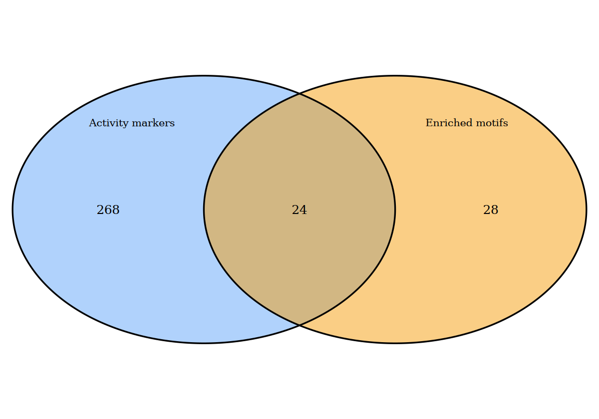

💡 Note
The Venn diagram example here displays the overlap of transcription factors (TFs) computed from two different dimensions, aiming to identify high-confidence core regulators:
Activity markers (blue region): TFs whose activity is significantly elevated in the current cell cluster or experimental group, directly identified through differential analysis (wilcoxauc) based on the ChromVAR-computed TF activity matrix.
Enriched motifs (orange region): Transcription factors obtained by performing sequence enrichment analysis using FindMotifs on the specifically accessible regions (differential Peaks) of the current cell cluster or experimental group.
Intersection (Overlap): Transcription factors satisfying both conditions simultaneously. This represents TFs whose binding motifs are not only abundantly found in specifically accessible regions but also exhibit significantly up-regulated overall binding activity at the genome-wide level. TFs in the intersection are highly likely to be the core regulators driving the current cell state or responding to experimental conditions.

ATAC + RNA Multi-omics: Motif Analysis ​

1. Tutorial Overview ​

2. Input File Preparation ​

2.1 Input File Requirements ​

Example Directory Structure ​

2.2 Definition of Core Helper Functions ​

3. Data Loading and Preprocessing ​

3.1 Loading the Seurat Object and Metadata ​

3.2 Cell Type Selection and Downsample Balancing ​

3.3 Modifying Fragment File Paths ​

4. Motif Activity Analysis ​

4.1 Reference Genome Processing ​

4.2 Motif Data Acquisition ​

4.3 Motif Activity Analysis ​

4.4 Global TF Activity–Expression Correlation Analysis ​

4.5 Differential TF Activity Analysis Across Cell Populations / Groups ​

5. Motif Enrichment Analysis ​

5.1 Differential Peak Dataset Preparation ​

5.2 Motif Enrichment Analysis and Visualization of Differential Peaks ​

5.3 Motif Enrichment Result Summarization ​

5.4 TF Activity vs DiffPeak Enriched Motif Overlap Analysis (Venn Diagram) ​