ATAC + RNA Multi-omics: Multi-Sample Integration Analysis Based on Signac

Author: SeekGene

Time: 24 min

Words: 4.8k words

Updated: 2026-07-07

Reads: 0 times

1. Tutorial Overview

This tutorial is built on single-cell multi-omics analysis tools including Seurat + Signac + Harmony, and is designed to perform multi-sample integration analysis, batch effect correction, joint clustering, and cell-type annotation on SeekArc single-cell multi-omics data (RNA + ATAC).

This tutorial is intended for single-cell datasets where each cell simultaneously carries transcriptomic expression information and chromatin accessibility information. By separately integrating the RNA and ATAC modalities across multiple samples and combining multi-modal analysis strategies, it achieves the following core analytical objectives:

• Multi-Sample Integration: Unified processing of single-cell multi-omics data from different samples, reducing the impact of batch differences on downstream analyses.
• Dual-Modality Joint Analysis: Simultaneously leveraging RNA expression features and ATAC open-chromatin features to more comprehensively characterize cellular states and biological heterogeneity.
• Batch Effect Correction: Providing integration methods based on CCA and Harmony to correct technical biases across different samples.
• Clustering and Dimensionality Reduction Visualization: Constructing cell similarity networks based on three dimensionality reduction strategies — RNA (PCA), ATAC (LSI), and WNN multi-modal fusion — followed by nonlinear dimensionality reduction (UMAP/t-SNE) and multi-resolution clustering, enabling cross-validation of results.
• Cell-Type Annotation: Providing biological interpretation and cell-type labeling of clustering results by combining marker gene expression patterns and genomic region accessibility.

suppressPackageStartupMessages({
  library(Seurat)
  library(Signac)
  library(EnsDb.Hsapiens.v86)
  library(BSgenome.Hsapiens.UCSC.hg38)
  library(biovizBase)
  #library(BSgenome.Mmusculus.UCSC.mm10)
  #library(EnsDb.Mmusculus.v79)
  library(dplyr)
  library(ggplot2)
  library(patchwork)
  library(harmony)
})


set.seed(1234)

options(future.globals.maxSize = 8000 * 1024^2)  # 8GB

my36colors <-c( '#E5D2DD', '#53A85F', '#F1BB72', '#F3B1A0', '#D6E7A3', '#57C3F3', '#476D87',
                '#E95C59', '#E59CC4', '#AB3282', '#23452F', '#BD956A', '#8C549C', '#585658',
                '#9FA3A8', '#E0D4CA', '#5F3D69', '#C5DEBA', '#58A4C3', '#E4C755', '#F7F398',
                '#AA9A59', '#E63863', '#E39A35', '#C1E6F3', '#6778AE', '#91D0BE', '#B53E2B',
                '#712820', '#DCC1DD', '#CCE0F5', '#CCC9E6', '#625D9E', '#68A180', '#3A6963',
                '#968175', "#6495ED", "#FFC1C1",'#f1ac9d','#f06966','#dee2d1','#6abe83','#39BAE8','#B9EDF8','#221a12',
                '#b8d00a','#74828F','#96C0CE','#E95D22','#017890')

# --- Input Parameter Configuration ---

## file_path: Path to the input Seurat object
file_path = "/path/to/sampleDir"

# integration_method: Algorithm used for integration. This tutorial provides two data integration methods: CCA and Harmony; only one can be selected. The purpose of integration is to remove batch effects between samples.
integration_method = "harmony" 

## sample_name: Names of samples to be analyzed.
##   - Multi-sample integration mode: Fill in multiple sample names separated by commas (e.g., "sample1,sample2,sample3"). The system will automatically trigger multi-sample integration and batch correction.
sample_names = c('pbmc_1', 'pbmc_2')

2. Input File Preparation

2.1 Input File Requirements

Please ensure that each sample is organized according to a unified directory structure. Each sample should be placed in its own folder; the folder name is recommended to be the sample ID directly, e.g., pbmc_1, pbmc_2, etc. Each sample directory should contain the following:

• filtered_feature_bc_matrix: scRNA-seq expression matrix directory, containing barcodes.tsv.gz, features.tsv.gz, and matrix.mtx.gz.
• filtered_peaks_bc_matrix: scATAC-seq peak accessibility matrix directory, containing barcodes.tsv.gz, features.tsv.gz, and matrix.mtx.gz.
• {sampleID}_A_fragments.tsv.gz: ATAC fragment file, used for downstream construction of ChromatinAssay, computation of TSS enrichment, nucleosome signal, and related analyses.
• {sampleID}_A_fragments.tsv.gz.tbi: Index file corresponding to the ATAC fragment file.

2.2 Example Directory Structure

pbmc_1/
├── filtered_feature_bc_matrix/
│   ├── barcodes.tsv.gz
│   ├── features.tsv.gz
│   └── matrix.mtx.gz
├── filtered_peaks_bc_matrix/
│   ├── barcodes.tsv.gz
│   ├── features.tsv.gz
│   └── matrix.mtx.gz
├── pbmc_1_A_fragments.tsv.gz
└── pbmc_1_A_fragments.tsv.gz.tbi

pbmc_2/
├── filtered_feature_bc_matrix/
│   ├── barcodes.tsv.gz
│   ├── features.tsv.gz
│   └── matrix.mtx.gz
├── filtered_peaks_bc_matrix/
│   ├── barcodes.tsv.gz
│   ├── features.tsv.gz
│   └── matrix.mtx.gz
├── pbmc_2_A_fragments.tsv.gz
└── pbmc_2_A_fragments.tsv.gz.tbi

2.3 Notes

• The directory structure across all samples must remain consistent; otherwise, the program may report errors during batch reading.
• The sample names filled in sample_names must exactly match the actual folder names.
• The ATAC fragment file and its index file must exist as a pair; otherwise, ChromatinAssay cannot be constructed properly.
• RNA and ATAC data should come from the same batch of cells or the same multi-omics experimental system to ensure accuracy of downstream joint analyses.

---

3. Data Loading and Preprocessing

Before commencing the multi-sample integration analysis, the genome annotation must be loaded, and the RNA and ATAC data for each sample must be read and used to build analysis objects. The goal of this step is: to construct a Seurat object containing both RNA and ATAC modalities for each sample, and store them uniformly in a list for subsequent quality control, integration, and clustering analyses.

3.1 Obtaining Gene Annotation Information

First, read the reference genome annotation from the EnsDb database and generate an annotation object. This annotation contains gene positions, transcription start sites (TSS), and other information, which can be used for downstream TSS enrichment analysis, gene activity analysis, and peak annotation.

This example uses the human annotation database EnsDb.Hsapiens.v86, unifies chromosome names to the format with the chr prefix, and specifies the reference genome version as hg38. This ensures consistency between the annotation and the chromosome naming in the ATAC data, avoiding errors in downstream analyses.

suppressWarnings({
  suppressMessages({
    annotation <- GetGRangesFromEnsDb(ensdb = EnsDb.Hsapiens.v86)
    seqlevels(annotation) <- paste0('chr', seqlevels(annotation))
    genome(annotation) <- 'hg38'
  })
})

3.2 Data Reading and Preprocessing

This step mainly completes the reading of multi-sample RNA and ATAC data, loading of genome annotation information, and construction of multi-omics Seurat objects, preparing for subsequent quality control, integration analysis, and clustering analysis. It includes the following stages:

1. Reading Multi-Sample RNA Data: Sequentially read the filtered_feature_bc_matrix expression matrix of each sample and create a Seurat object for the RNA assay.
2. Reading Multi-Sample ATAC Data: Read the filtered_peaks_bc_matrix accessibility matrix and fragment file for each sample, construct the ATAC assay, and add it to the corresponding Seurat object. In particular, the annotation genome annotation information mentioned above is incorporated when constructing the ATAC assay, to support downstream ATAC-related analyses.
3. Saving the Multi-Omics Object List: Save the RNA + ATAC Seurat object constructed for each sample into seurat_list, for use in downstream multi-sample integration analysis.

seurat_list <- list()
for(sample in sample_names){

  atac_path <- file.path(file_path, sample, 'filtered_peaks_bc_matrix')
  rna_path <- file.path(file_path, sample, 'filtered_feature_bc_matrix')
  frag_path <- file.path(file_path, sample, paste0(sample, '_A_fragments.tsv.gz'))
  
  rna_counts <- Read10X(data.dir = rna_path)

  obj <- CreateSeuratObject(
    counts = rna_counts,
    assay = "RNA")
  
  obj$Sample <- sample
  rm(rna_counts)
  gc()
  
  atac_counts <- Read10X(data.dir = atac_path)
  atac_counts <- atac_counts[Matrix::rowSums(atac_counts > 0) >= 3, ]   

  ChromatinAssay <- CreateChromatinAssay(
    counts = atac_counts,
    sep = c(":", "-"),
    fragments = frag_path,
    annotation = annotation
  )
  
  obj[["ATAC"]] <- ChromatinAssay
  rm(atac_counts, ChromatinAssay)
  gc()
  
  seurat_list[[sample]] <- obj
}

4. Data Quality Control

4.1 Quality Metric Computation

After reading multi-sample data, quality control must be performed separately on each sample to remove low-quality cells and ensure the reliability of downstream integration analysis results. This step computes commonly used quality metrics for both RNA and ATAC modalities.

RNA Quality Metrics:

• percent.mt: Proportion of mitochondrial genes, typically used to assess cell status; abnormally high values may indicate low-quality or damaged cells.

ATAC Quality Metrics:

• TSS.enrichment: TSS enrichment score, evaluating the degree to which open-chromatin signal is enriched around transcription start sites.
• nucleosome_signal: Nucleosome signal, reflecting fragment distribution characteristics; generally, lower is better.

suppressWarnings({
  suppressMessages({
      for(i in names(seurat_list)){
          seurat_list[[i]][["percent.mt"]] <- PercentageFeatureSet(seurat_list[[i]], pattern = "^MT-")
          DefaultAssay(seurat_list[[i]]) <- "ATAC"
          seurat_list[[i]] <- TSSEnrichment(object = seurat_list[[i]], fast = FALSE) 
          seurat_list[[i]] <- NucleosomeSignal(object = seurat_list[[i]])
      }
  })
})

Note: The quality metrics for seekARC dual-omics data also include nCount_RNA, nCount_ATAC, nFeature_RNA, nFeature_ATAC, and others, which are automatically generated during Seurat object construction in the preceding step.

4.2 Quality Metric Visualization

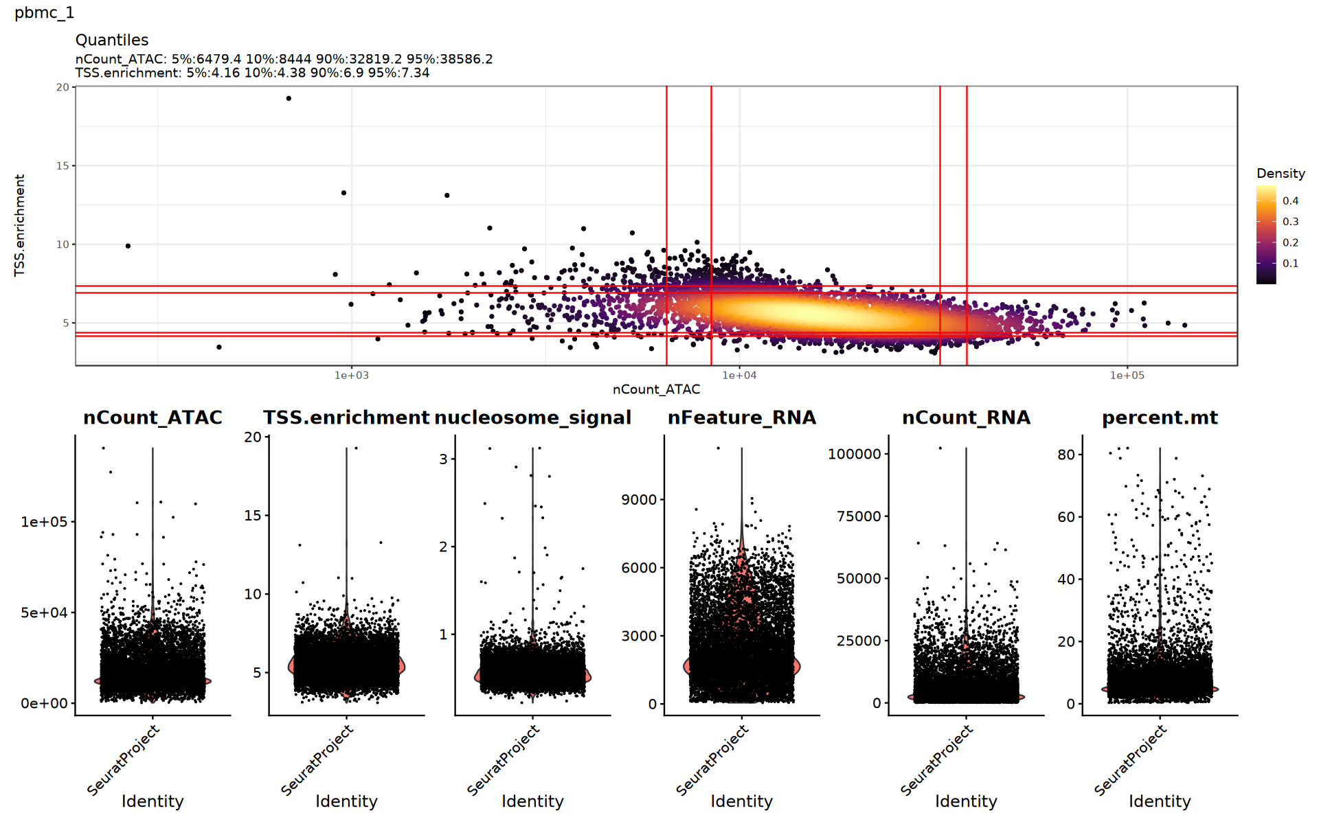
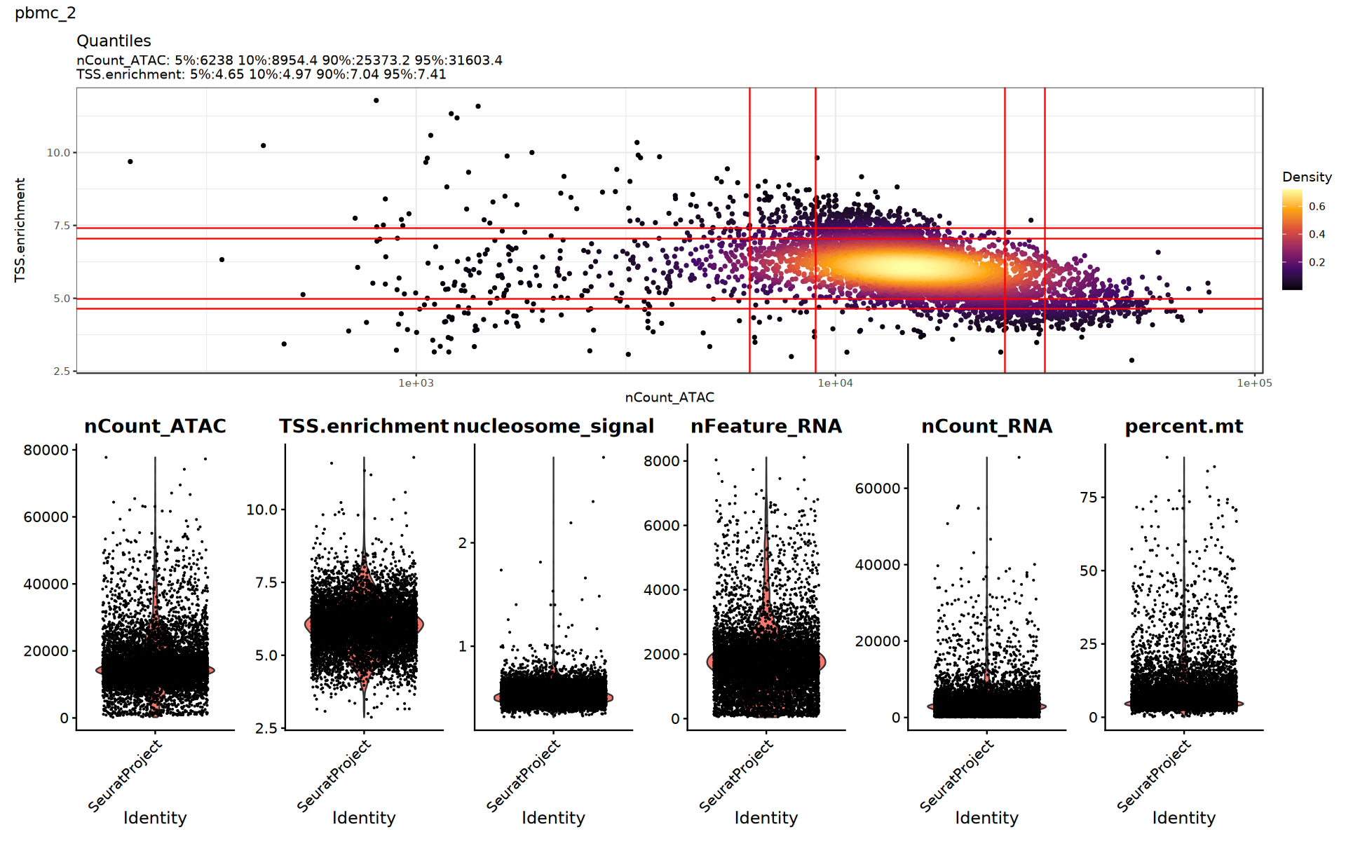
After computing the quality metrics, violin plots and scatter plots can be used to inspect the distribution of each metric, helping to assess data quality and select appropriate filtering thresholds.

It is recommended to focus on the following:

• Whether there are obvious outliers, long-tailed distributions, or bimodal distributions;
• Whether the distributions of quality metrics are consistent across different samples;
• Reasonable adjustment of filtering thresholds based on the visualization results, to obtain clearer downstream clustering and UMAP results.

options(repr.plot.width = 16, repr.plot.height = 10)
suppressWarnings({
for (sample_name in names(seurat_list)) {
  seurat_obj <- seurat_list[[sample_name]]
  p1=DensityScatter(seurat_obj, x = 'nCount_ATAC', y = 'TSS.enrichment', log_x = TRUE, quantiles = TRUE)
  p2=VlnPlot(
      object = seurat_obj,
      features = c('nCount_ATAC', 'TSS.enrichment',  'nucleosome_signal',"nFeature_RNA", "nCount_RNA", "percent.mt"),
      pt.size = 0.1,
      ncol = 6
  )
 print(p1 / p2 + plot_annotation(title = sample_name))
}
})

4.3 Filtering Out Low-Quality Cells

Based on the quality metrics computed above, low-quality cells are filtered out to remove abnormal cells and improve the reliability of downstream analysis results. Specific filtering thresholds should be set according to the actual sample conditions, typically guided by the violin plots and scatter plots of the quality metrics.

for(i in names(seurat_list)){
  cells_before <- ncol(seurat_list[[i]])
  
  seurat_list[[i]] <- subset(
    seurat_list[[i]],
    subset = nFeature_RNA > 200 &
             nFeature_RNA < 8000 &
             nCount_RNA > 500 &
             nCount_RNA < 30000 &
             percent.mt < 20 &
             nCount_ATAC > 500 &
             nCount_ATAC < 50000 &
             TSS.enrichment > 1 &
             nucleosome_signal < 1
  )
  
  cells_after <- ncol(seurat_list[[i]])
}

5. Computing Shared Peaks Across Samples

Since different samples typically undergo peak calling separately, the ATAC peak sets across samples are not completely identical. To carry out multi-sample integration analysis, the peaks from all samples must first be merged to construct a unified shared peak set, and the ATAC matrix for each sample must be regenerated based on this unified set.

This step mainly includes the following:

1. Merging Peaks from All Samples: Extract the peak interval information from each sample and merge them into a unified peak set.
2. Filtering Peak Lengths: Remove peaks that are too short or too long; typically, intervals with lengths between 20 bp and 10 kb are retained.
3. Re-quantifying Shared Peaks: Using the unified peak set as the basis, re-compute ATAC counts for each sample, ensuring that different samples use the same feature space.

all_peaks <- lapply(seurat_list, function(x) {
  DefaultAssay(x) <- "ATAC"
  granges(x@assays$ATAC)
})

gr_list <- GRangesList(all_peaks)
all_granges <- unlist(gr_list, use.names = FALSE)
combined.peaks <- reduce(x = all_granges)

peakwidths <- width(combined.peaks)
common_peaks <- combined.peaks[peakwidths < 10000 & peakwidths > 20]

seurat_list <- lapply(seurat_list, function(x) {
  combined_counts <- FeatureMatrix(
    fragments = Fragments(x@assays$ATAC),
    features = common_peaks,
    cells = colnames(x)
  )
  
  combined_peaks_assay <- CreateChromatinAssay(
    counts = combined_counts,
    fragments = Fragments(x@assays$ATAC),
    annotation = Annotation(x@assays$ATAC)
  )

  x[["combinedpeaks"]] <- combined_peaks_assay
  DefaultAssay(x) <- "combinedpeaks"
  x[["ATAC"]] <- NULL
  return(x)
})

6. Multi-Sample Merging

After completing data preprocessing for each sample, multiple samples need to be merged into a single Seurat object as input for subsequent batch correction and multi-omics integration analyses.

The main purposes of this step are:

• Unifying data from multiple samples into the same object;
• Preparing for subsequent batch effect correction, dimensionality reduction, and clustering analysis;
• Facilitating comparison of data differences before and after integration.

Note that this step only performs sample merging and does not involve batch effect correction. The merged object still retains the original feature information of each sample; subsequent standard preprocessing such as normalization, feature selection, and dimensionality reduction is still typically required.

suppressWarnings({
  suppressMessages({
      obj_merge <- merge(seurat_list[[1]], seurat_list[-1], merge.data = FALSE)
      DefaultAssay(obj_merge) <- "RNA" 
      obj_merge <- NormalizeData(obj_merge)
      obj_merge <- FindVariableFeatures(obj_merge, nfeatures = 2000)
      obj_merge <- ScaleData(obj_merge)
      obj_merge <- RunPCA(obj_merge)
      obj_merge <- RunUMAP(obj_merge, reduction = "pca", dims = 2:30,reduction.name="rnaumap")
      DefaultAssay(obj_merge) <- "combinedpeaks"
      obj_merge <- FindTopFeatures(obj_merge, min.cutoff = 10)
      obj_merge <- RunTFIDF(obj_merge)
      obj_merge <- RunSVD(obj_merge)
      obj_merge <- RunUMAP(obj_merge, reduction = "lsi", dims = 2:30,reduction.name="atacumap")
        })
})

P1=DimPlot(obj_merge, reduction = "rnaumap", group.by = "Sample")
P2=DimPlot(obj_merge, reduction = "atacumap", group.by="Sample")

options(repr.plot.width=17, repr.plot.height=8)
patchwork::wrap_plots(P1, P2, ncol = 2)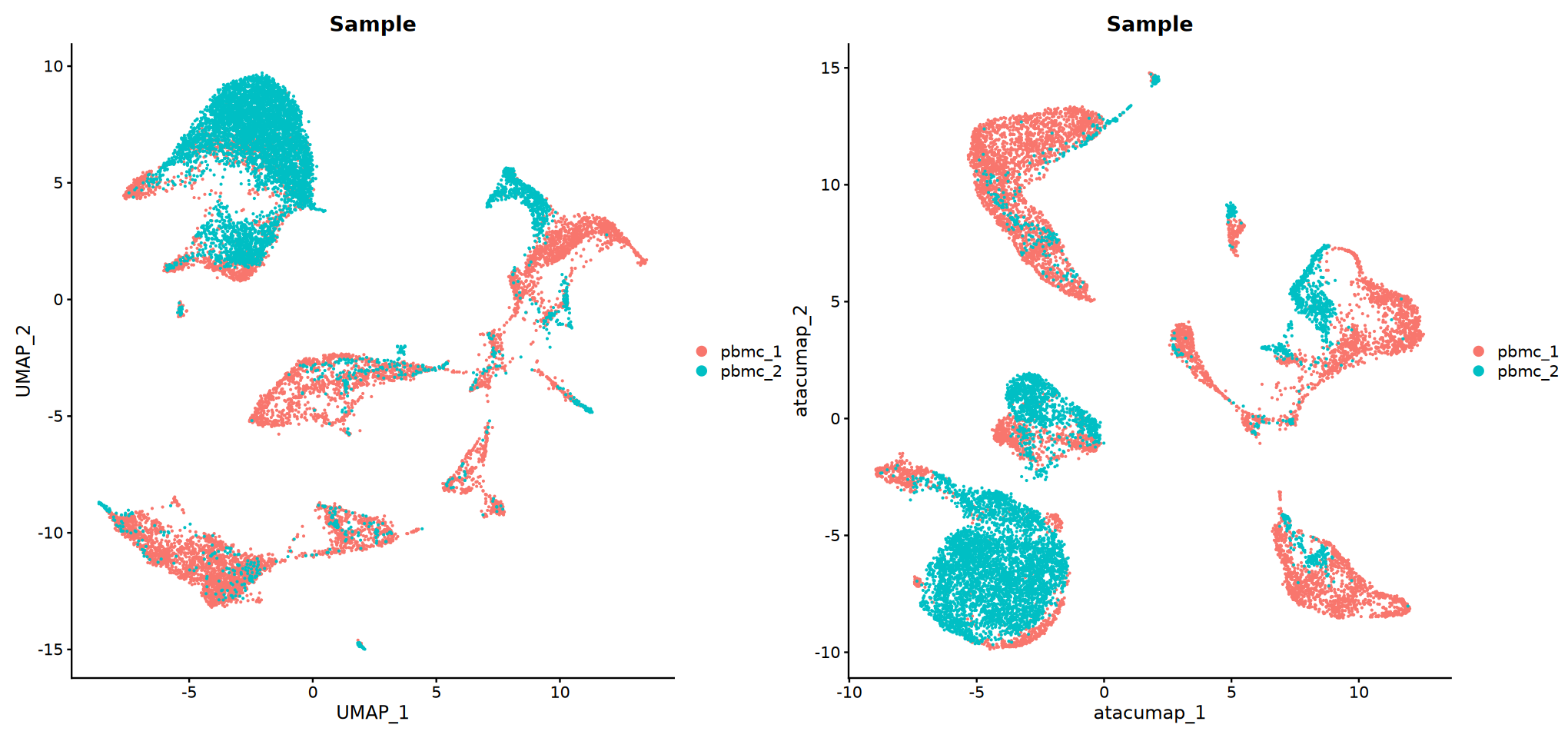

💡 NoteNote: At the current stage, only preliminary data merging has been completed (scRNA and scATAC data merged by sample separately); batch correction has not yet been performed. The left panel shows the dimensionality reduction plot of the merged RNA data; the right panel shows that of the merged ATAC data. The distributional differences between samples shown in the plots can preliminarily reflect the strength of the batch effect: if cells of the same type are clearly separated due to different sample origins, this indicates the presence of a batch effect and subsequent correction is required; if the cell distributions between samples are highly overlapping, the batch correction step may be skipped. In practice, most multi-sample data exhibit batch effects of varying degrees, and correction is typically necessary.

7. Data Integration

After completing multi-sample merging, batch differences across samples need to be further corrected. For SeekArc single-cell multi-omics data, the RNA and ATAC modalities must each be integrated separately before being used in downstream joint analyses.

7.1 Selection of Integration Method

This tutorial provides two commonly used batch correction methods: CCA and Harmony.

CCA (Canonical Correlation Analysis) Integration:

• Based on Seurat's anchor integration strategy, achieving data alignment by identifying shared features across samples;
• Suitable for cases where differences between samples are obvious and batch effects are strong;
• Relatively high computational cost, usually with longer runtime.

Harmony Integration:

• Directly performs batch correction in an existing dimensionality-reduced space, such as the RNA PCA space or the ATAC LSI space;
• Runs faster, suitable for scenarios with a large number of samples or large data scales; typically preserves biological differences well while reducing batch effects;
• More suitable for multi-sample integration analysis of data from the same platform and of the same type.

Notes

• RNA and ATAC need to be integrated separately before being used in downstream multi-modal joint analysis.
• In practice, it is recommended to comprehensively evaluate integration quality by combining the UMAP mixing effect, clustering results, and known biological information.

7.2 Starting RNA Data Integration

if(integration_method == "CCA"){
    rnaintegratedumap="rnaintegratedumap"
    rnaintegratedtsne="rnaintegratedtsne"
    suppressWarnings({  
        suppressMessages({
            objs <- lapply(seurat_list, function(x) {
                DefaultAssay(x) <- "RNA"
                return(x)
            })
            integrate_cca <- function(objs) {
                objs <- lapply(objs, function(x) {
                    x <- NormalizeData(x, verbose = FALSE)
                    x <- FindVariableFeatures(x,nfeatures = 2000,selection.method = "vst")
                    return(x)
                })
                features <- Seurat::SelectIntegrationFeatures(object.list = objs)
                anchors <- Seurat::FindIntegrationAnchors(
                    object.list = objs,
                    anchor.features = features
                ) 
                obj <- Seurat::IntegrateData(anchorset = anchors)
                DefaultAssay(obj) <- "integrated"
                obj <- ScaleData(obj, verbose = FALSE)
                obj <- RunPCA(obj, verbose = FALSE)
                obj <- RunUMAP(obj, reduction = "pca",reduction.name=rnaintegratedumap, dims = 1:30)
                #obj <- RunTSNE(obj, reduction = "pca", reduction.name=rnaintegratedtsne,dims = 1:30, check_duplicates = FALSE)
                return(obj)
            }
            obj_integrated <- integrate_cca(seurat_list)
        })
    })      
} else {
    rnaintegratedumap="rnaharmonyumap"
    rnaintegratedtsne="rnaharmonytsne"
    integrate_harmony <- function(obj) {
        DefaultAssay(obj) <- "RNA"
        obj <- RunHarmony(obj, "Sample")
        obj <- RunUMAP(obj, reduction = "harmony",reduction.name=rnaintegratedumap,dims = 1:30)
        #obj <- RunTSNE(obj, reduction = "harmony",reduction.name=rnaharmonytsne,dims = 1:30,check_duplicates = FALSE)
        return(obj)
    }
    suppressWarnings({
        suppressMessages({
            obj_integrated = integrate_harmony(obj_merge)
        })
    }) 
}

options(repr.plot.width=10, repr.plot.height=8)
DimPlot(obj_integrated, reduction = rnaintegratedumap, group.by = "Sample")
options(repr.plot.width=16, repr.plot.height=8)
DimPlot(obj_integrated, reduction = rnaintegratedumap, split.by = "Sample")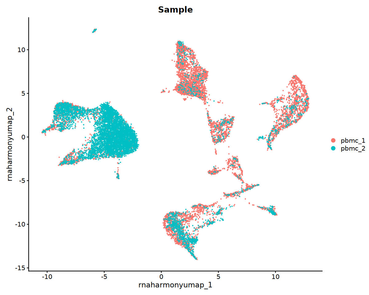

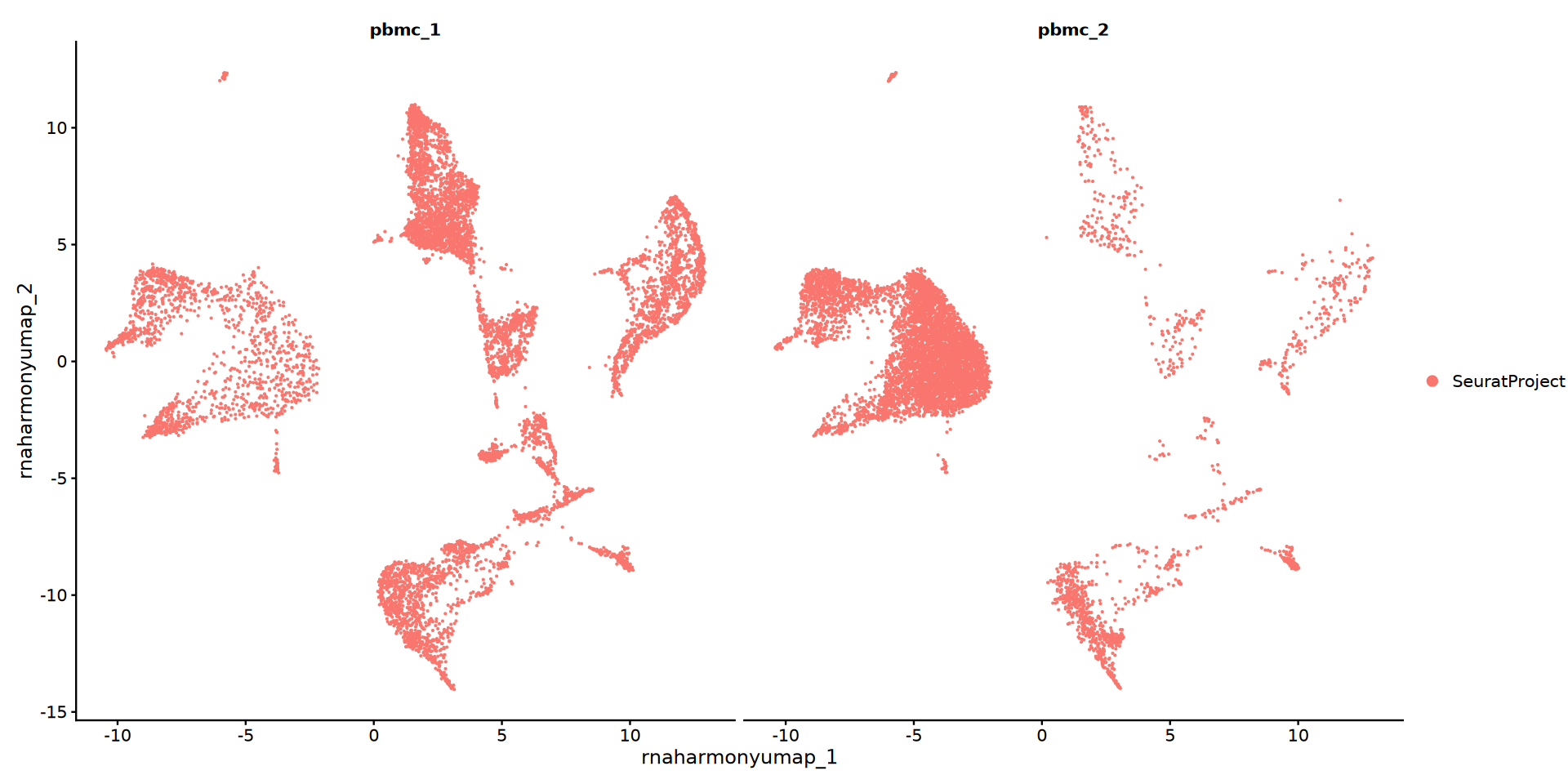
💡 NoteNote: This plot displays the distribution of RNA data after batch correction. When evaluating the batch-effect removal effectiveness, observation should be performed within the same cell type: if cells of the same type have achieved mixed distribution across samples, batch correction is effective; if cells of the same type still separate into clusters by sample, batch removal is incomplete. Note that evaluation must be performed at the cell-type level, not based on the overall UMAP distribution, because there may be genuine biological differences between samples (e.g., differences in cell-type composition or proportions).

7.3 ATAC Data Integration

if(integration_method == "CCA"){
    atacintegratedumap="atacintegratedumap"
    atacintegratedtsne="atacintegratedtsne"
    integrated_lsi="integrated_lsi"
    options(future.globals.maxSize = 20 * 1024^3)
    integrate_atac_cca <- function(object.list){
        object.list <- lapply(object.list, function(x) {
            DefaultAssay(x)="combinedpeaks"
            x=RunTFIDF(x)
            x=FindTopFeatures(x, min.cutoff = 5)
            x=RunSVD(x)
            return(x)
        })
        anchors <- FindIntegrationAnchors(
            object.list = object.list,
            anchor.features = rownames(obj_merge),
            reduction = "rlsi",
            dims = 2:30
        )
        integrated <- IntegrateEmbeddings(
            anchorset = anchors,
            reductions = obj_merge[["lsi"]],
            new.reduction.name = "integrated_lsi",
            dims.to.integrate = 1:30)
        integrated<- RunUMAP(integrated, reduction = integrated_lsi, dims = 2:30,reduction.name=atacintegratedumap)
        integrated<- RunTSNE(integrated, reduction = integrated_lsi, dims = 2:30,reduction.name=atacintegratedtsne)
        return(integrated)
    }
    suppressWarnings({
        suppressMessages({
            integrated_atac <- integrate_atac_cca(seurat_list)
        })
    })  
    obj_integrated[[integrated_lsi]] <- integrated_atac[[integrated_lsi]]
    obj_integrated[[atacintegratedumap]] <- integrated_atac[[atacintegratedumap]]
    obj_integrated[[atacintegratedtsne]] <- integrated_atac[[atacintegratedtsne]]
    DefaultAssay(obj_integrated) <- "integrated"
} else {
    atacintegratedumap="atacharmonyumap"
    atacintegratedtsne="atacharmonytsne"
    integrated_lsi="harmonylsi"
    atac_integrate_harmony <- function(obj) {
        library(harmony)
        DefaultAssay(obj) <- "combinedpeaks"
        obj<- RunHarmony(
            object = obj,
            group.by.vars = 'Sample',
            reduction = 'lsi',
            assay.use = 'combinepeaks',
            reduction.save = integrated_lsi,
            project.dim = FALSE
        )
        obj <- RunUMAP(obj,reduction = integrated_lsi,reduction.name=atacintegratedumap, dims = 2:50)
        #obj <- RunTSNE(obj, reduction = integrated_lsi,reduction.name=atacintegratedtsne,dims = 2:50,check_duplicates = FALSE)
        return(obj)
    }
    suppressWarnings({
        suppressMessages({
            obj_integrated=atac_integrate_harmony(obj_integrated)
        })
    })
}

options(repr.plot.width=10, repr.plot.height=8)
DimPlot(obj_integrated, reduction = atacintegratedumap, group.by = "Sample")
options(repr.plot.width=16, repr.plot.height=8)
DimPlot(obj_integrated, reduction = atacintegratedumap, split.by = "Sample")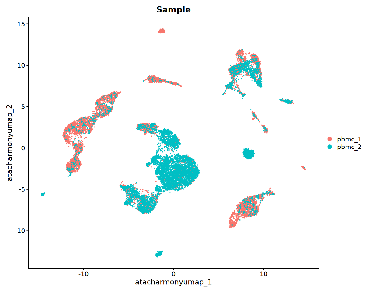

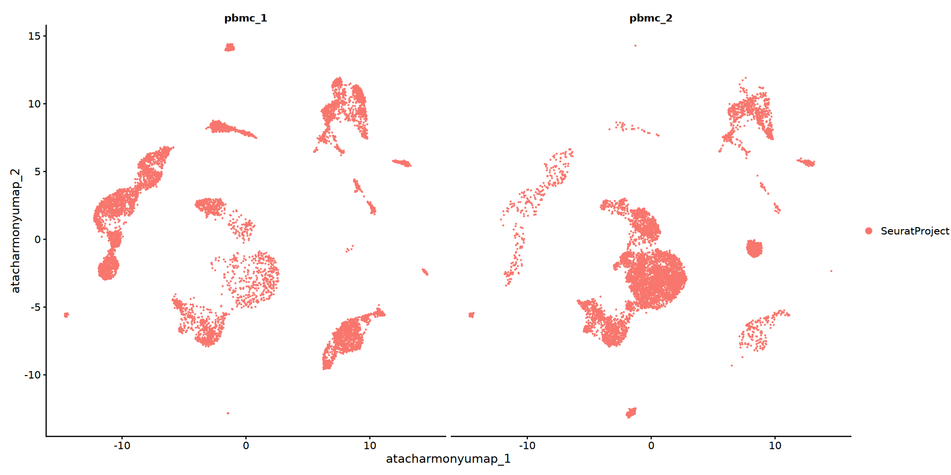
💡 NoteNote: This plot displays the distribution of ATAC data after batch correction. The method for evaluating batch correction effectiveness is the same as described above.

8. Nonlinear Dimensionality Reduction and Clustering Analysis

Having completed the integration and batch correction of RNA and ATAC data, we can further reveal the complex relationships of cells in high-dimensional space using nonlinear dimensionality reduction methods. Commonly used nonlinear techniques include t-SNE and UMAP, which map high-dimensional data into two- or three-dimensional space to facilitate visualization of cell subpopulation structure.

Three Clustering Strategies

1. RNA Clustering: Based on gene expression similarity, constructing a nearest-neighbor graph using the PCA results of the RNA-seq data.
2. ATAC Clustering: Based on chromatin accessibility similarity, constructing a nearest-neighbor graph using the LSI results of the ATAC-seq data.
3. WNN Clustering: Integrating both modalities (recommended), based on the weighted nearest neighbor algorithm, comprehensively considering the contributions of RNA and ATAC modalities to cell similarity.

Note:

Before performing dimensionality reduction and clustering, the optimal number of dimensions for both RNA and ATAC data must be determined separately to avoid noise interference or information loss.

options(repr.plot.width = 13, repr.plot.height = 7)
DepthCor(obj_integrated, reduction = integrated_lsi,n = 50)
#DepthCor(obj_integrated，reduction = integrated_lsi, n = 50)

output

Warning message in grid.Call(C_textBounds, as.graphicsAnnot(x$label), x$x, x$y, :
"font width unknown for character 0x9"
Warning message in grid.Call.graphics(C_text, as.graphicsAnnot(x$label), x$x, x$y, :
"font width unknown for character 0x9"

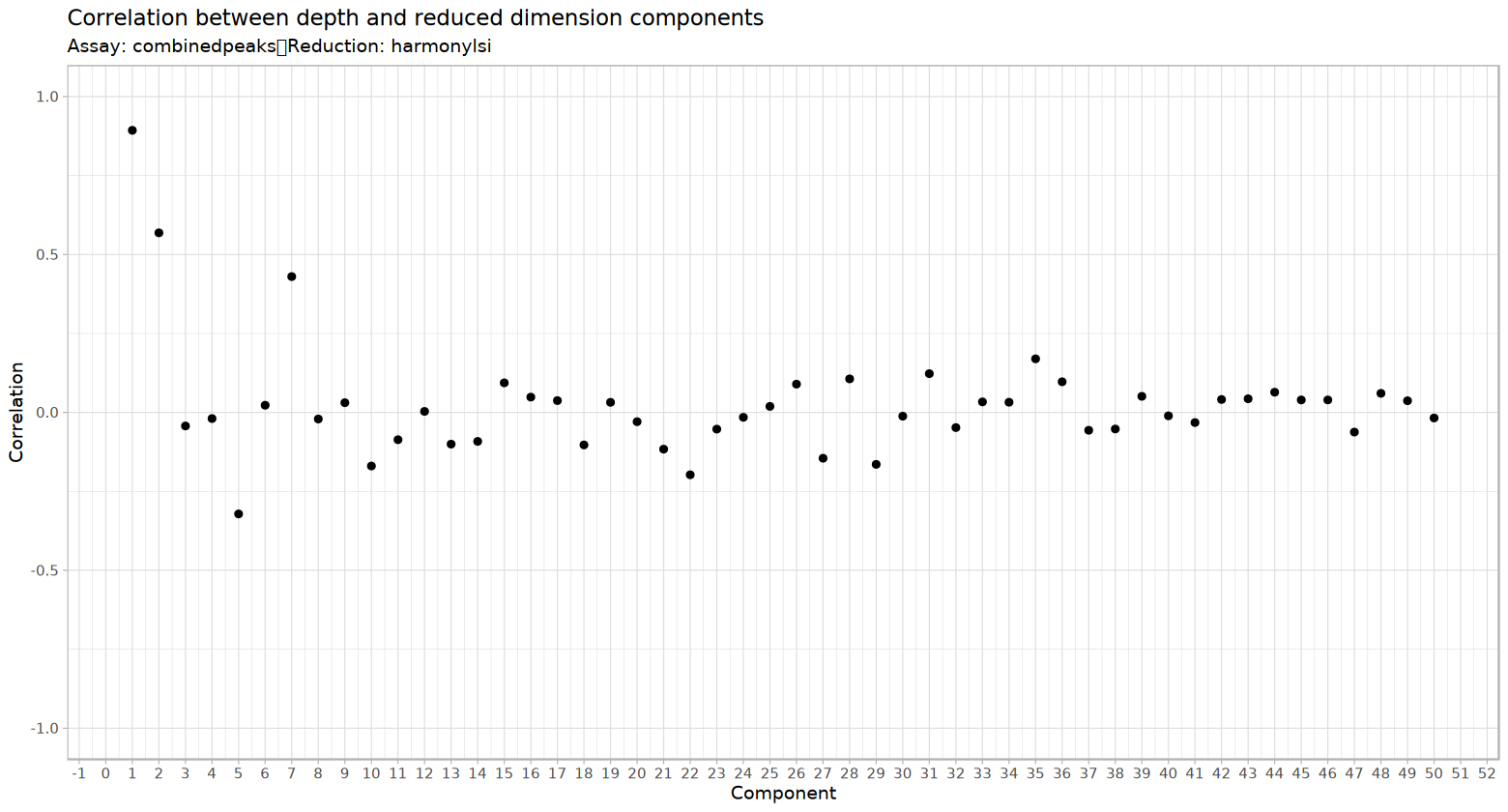
💡 NoteLSI Dimension Selection: In ATAC data analysis, the first LSI component sometimes more strongly reflects technical factors such as sequencing depth rather than biological variation. Therefore, it is recommended to use DepthCor() to evaluate the correlation between each LSI dimension and sequencing depth. If the first dimension is found to be significantly correlated with sequencing depth, it is typically excluded from downstream neighbor search, UMAP dimensionality reduction, and clustering analyses. Sometimes the second LSI may also be affected by sequencing depth; the actual choice of which dimensions to retain is determined based on this plot.

if(integration_method == "CCA"){
    tmp_reduction="pca"
}else{
    tmp_reduction="harmony"
}
ElbowPlot(obj_integrated, ndims =30, reduction = tmp_reduction)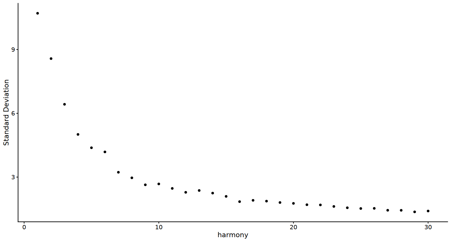

💡 NotePrincipal Component Dimension Selection: In RNA data analysis, ElbowPlot() can be used to inspect how much of the overall variation each principal component explains, thereby assisting in deciding the number of dimensions to retain for downstream analysis. Typically, after an obvious "elbow" in the curve, the contribution of additional principal components to variation gradually weakens, so the region around that elbow serves as a reference range for dimension truncation. Note that the true dimensionality of the data rarely has an absolute fixed threshold; it is recommended to combine the elbow plot, known biological information, and downstream results for a comprehensive decision. In practice, one may try different dimension numbers within adjacent ranges, such as 10, 15, or higher, and prefer a slightly larger dimension range to avoid missing potential biological signals.

8.1 WNN Joint Dimensionality Reduction and Clustering

# 寻找多模态邻居
obj_integrated <- FindMultiModalNeighbors(
          object = obj_integrated,
          reduction.list = list(tmp_reduction, integrated_lsi),
          dims.list = list(1:30, 3:50),
          modality.weight.name = "RNA.weight",
          verbose = TRUE)
obj_integrated <- RunUMAP(
          object = obj_integrated,
          nn.name = "weighted.nn",
          assay = "RNA",
          verbose = TRUE,
          reduction.name = "wnnintergratedumap"
      )
obj_integrated <- FindClusters(obj_integrated, 
                                     graph.name = "wknn", 
                                     algorithm = 3, resolution = 0.5, 
                                     verbose = TRUE)
options(repr.plot.width = 9, repr.plot.height = 7)

DimPlot(obj_integrated, reduction = "wnnintergratedumap", group.by = "wknn_res.0.5",label=T, cols = my36colors) + ggtitle("WNN")

8.2 Dimensionality Reduction and Clustering Based on RNA Data

obj_integrated <- FindNeighbors(object = obj_integrated, 
                                      reduction = 'pca',graph.name = "rnaneigobr", 
                                      dims = 1:30)
obj_integrated <- FindClusters(object = obj_integrated, 
                                     verbose = FALSE,graph.name = "rnaneigobr", 
                                     algorithm = 3, resolution = 0.5)

DimPlot(obj_integrated, reduction = rnaintegratedumap, group.by = "rnaneigobr_res.0.5",label=T, cols = my36colors) + ggtitle("RNA")

8.3 Dimensionality Reduction and Clustering Based on ATAC Data

obj_integrated <- FindNeighbors(object = obj_integrated, 
                                reduction = integrated_lsi, graph.name = "atacneigobr", 
                                dims = 2:30)
obj_integrated <- FindClusters(object = obj_integrated, 
                               verbose = FALSE, graph.name = "atacneigobr",
                               resolution = 0.5, algorithm = 3)

DimPlot(obj_integrated, reduction = atacintegratedumap, group.by = "atacneigobr_res.0.5",label=T, cols = my36colors) + ggtitle("ATAC")

9. Cell-Type Annotation

9.1 Inspecting Marker Gene Expression at the scRNA-seq Data Level

The example data in this tutorial are PBMC, so we have compiled common immune cell types and their corresponding marker gene sets. In actual analyses, marker genes should be customized according to sample origin and tissue type. Subsequently, a bubble plot can be used to inspect the expression of marker genes across different clusters, assisting in determining the cell type corresponding to each cluster.

pbmc_marker_integrated <- list(
  "Plasma Cells" = c("IGHG1", "IGKC"),
  "Monocytes" = c("VCAN", "FCN1", "TREM1"),
  "B cells" = c("MS4A1", "BACH2", "PAX5"),
  "CMP" = c("MPO"),
  "Pro B cells" = c("DNTT"),
  "Erythroblast" = c("ALAS2", "NFIA", "SOX6"),
  "T cells" = c("PLXNA4", "THEMIS", "ITK", "BCL11B"),
  "NK cells" = c("NCAM1", "KLRC3"),
  "Dividing B cells" = c("MKI67", "TOP2A"),
  "pDC" = c("RUNX2")
)

options(repr.plot.width=15, repr.plot.height=7)

DefaultAssay(obj_integrated)="RNA"
DotPlot(obj_integrated, 
        group.by = "wknn_res.0.5", 
        features = pbmc_marker_integrated,
        cols = c("#f8f8f8","#ff3472"),
       #dot.min = 0.05,
       dot.scale = 8)+
  RotatedAxis() + 
  scale_x_discrete("") + 
  scale_y_discrete("") +
  theme(
    axis.text.x = element_text(size = 12, face = "bold", 
                              angle = 45, hjust = 1, vjust = 1),
    axis.text.y = element_text(size = 12, face = "bold"),
    plot.title = element_text(size = 14, face = "bold", hjust = 0.5),
    legend.title = element_text(size = 10, face = "bold")
  ) +
  ggtitle("Marker Genes Expression") +
  labs(color = "Expression\nLevel")

output

Warning message:
"The \`facets\` argument of \`facet_grid()\` is deprecated as of ggplot2 2.2.0.
ℹ Please use the \`rows\` argument instead.
ℹ The deprecated feature was likely used in the Seurat package.
Please report the issue at ."

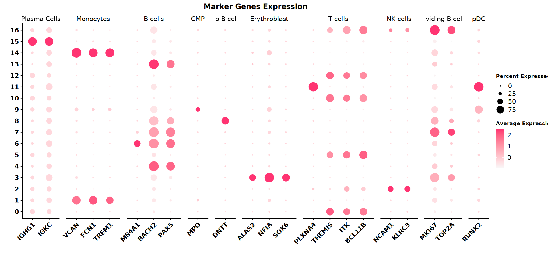
💡 NoteCell Annotation Note: In SeekArc single-cell dual-omics analysis, cell-type annotation is typically based on WNN multi-modal dimensionality reduction results, combined with the expression patterns of marker genes in the wknn clustering output, to determine the cell type of each cluster.

9.2 Inspecting Marker Gene Genomic Region Accessibility at the scATAC-seq Data Level

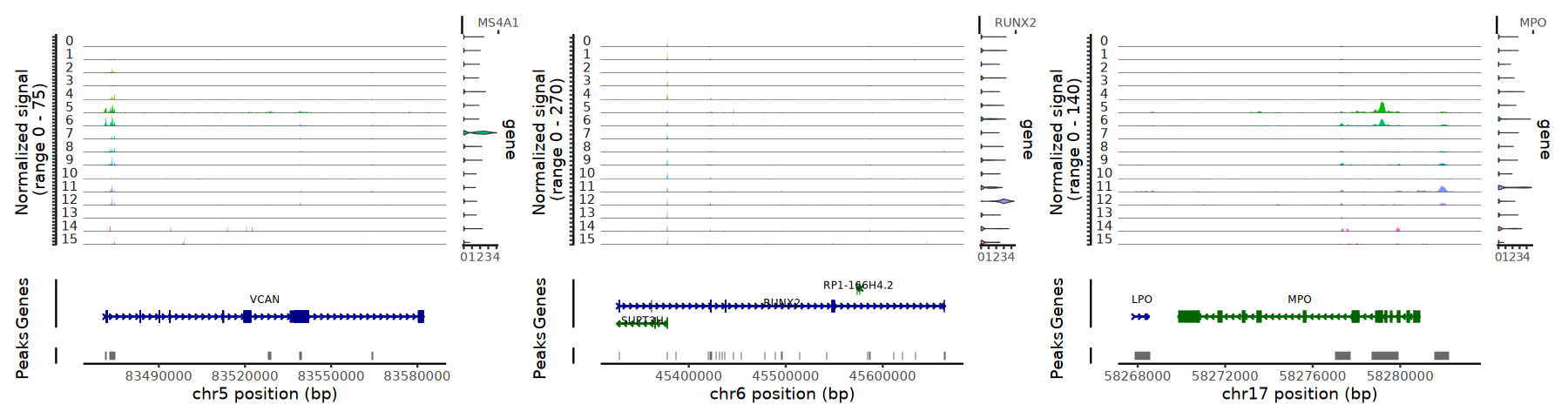
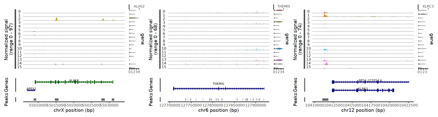
In addition to RNA expression, the accessibility of regulatory regions around marker genes can also be inspected at the scATAC-seq data level to further assist cell-type annotation. Typically, by combining the peak signal near the gene, the degree of chromatin accessibility, and the accessibility differences between different clusters, one can determine whether a specific marker gene is in an active regulatory state in the corresponding cell population.

DefaultAssay(obj_integrated) <- "combinedpeaks"
P1 <- CoveragePlot(
  object = obj_integrated,
  region = "VCAN",
  features = "MS4A1",
  expression.assay = "RNA",
  extend.upstream = 2000,
  extend.downstream = 2000
)

P2 <- CoveragePlot(
  object = obj_integrated,
  region = "RUNX2",
  features = "RUNX2",
  expression.assay = "RNA",
  extend.upstream = 2000,
  extend.downstream = 2000
)

P3 <- CoveragePlot(
  object = obj_integrated,
  region = "MPO",
  features = "MPO",
  expression.assay = "RNA",
  extend.upstream = 2000,
  extend.downstream = 2000
)

P4 <- CoveragePlot(
  object = obj_integrated,
  region = "ALAS2",
  features = "ALAS2",
  expression.assay = "RNA",
  extend.upstream = 2000,
  extend.downstream = 2000
)

P5 <- CoveragePlot(
  object = obj_integrated,
  region = "THEMIS",
  features = "THEMIS",
  expression.assay = "RNA",
  extend.upstream = 2000,
  extend.downstream = 2000
)

P6 <- CoveragePlot(
  object = obj_integrated,
  region = "KLRC3",
  features = "KLRC3",
  expression.assay = "RNA",
  extend.upstream = 2000,
  extend.downstream = 2000
)

options(repr.plot.width=15, repr.plot.height=4)
patchwork::wrap_plots(P1, P2, P3, ncol = 3)
patchwork::wrap_plots(P4, P5, P6, ncol = 3)

output

Warning message:
"Removed 54 rows containing missing values or values outside the scale range
(\`geom_segment()\`)."

Warning message:
"Removed 90 rows containing missing values or values outside the scale range
(\`geom_segment()\`)."

Warning message:
"Removed 11 rows containing missing values or values outside the scale range
(\`geom_segment()\`)."

Warning message:
"Removed 3 rows containing missing values or values outside the scale range
(\`geom_segment()\`)."

9.3 Cell-Type Labeling and Visualization

celltype_mapping <- c(
  "15" = "Plasma Cells",
  "1" = "Monocytes",
  "14" = "Monocytes",
  "4" = "B cells",
  "6" = "B cells",
  "13" = "B cells",
  "9" = "CMP",
  "8" = "Pro B cells",
  "3" = "Erythroblast",
  "0" = "T cells",
  "5" = "T cells",
  "10" = "T cells",
  "12" = "T cells",    
  "2" = "NK cells",
  "16" = "NK cells",
  "7" = "Dividing B cells",
  "11" = "pDC"
)
obj_integrated$celltype <- recode(
  obj_integrated$wknn_res.0.5,
  !!!celltype_mapping
)

p1 <- DimPlot(
  obj_integrated,
  reduction = "wnnintergratedumap",
  group.by = "celltype",
  label = TRUE,
  label.size = 3,
  cols = my36colors
) +
  ggtitle("celltype") +
  theme(legend.position = "bottom")

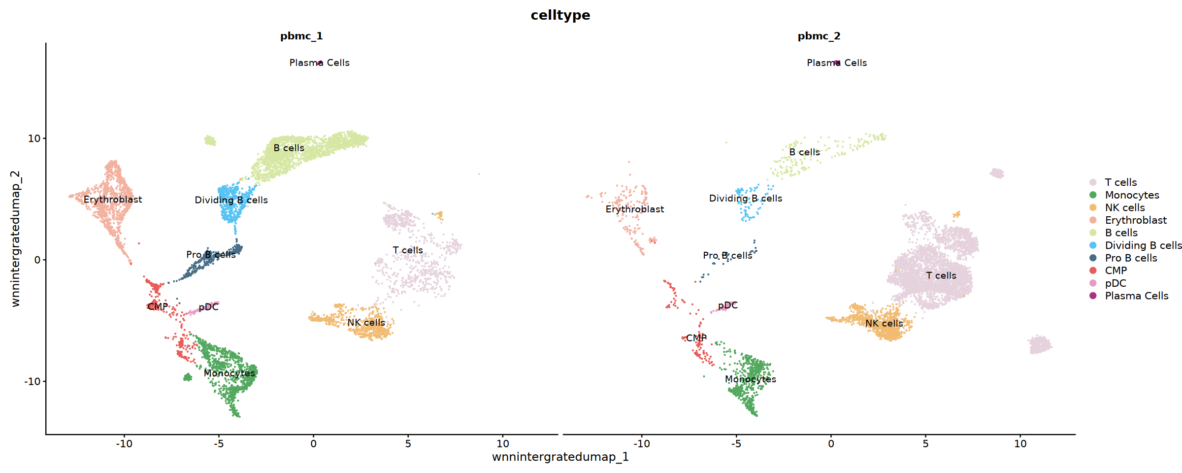
p2 <- DimPlot(
  obj_integrated,
  reduction = "wnnintergratedumap",
  group.by = "celltype",
  split.by = "Sample",
  cols = my36colors,
  ncol = 2,label=T
) 

options(repr.plot.width=10, repr.plot.height=8)
print(p1)
options(repr.plot.width=20, repr.plot.height=8)
print(p2)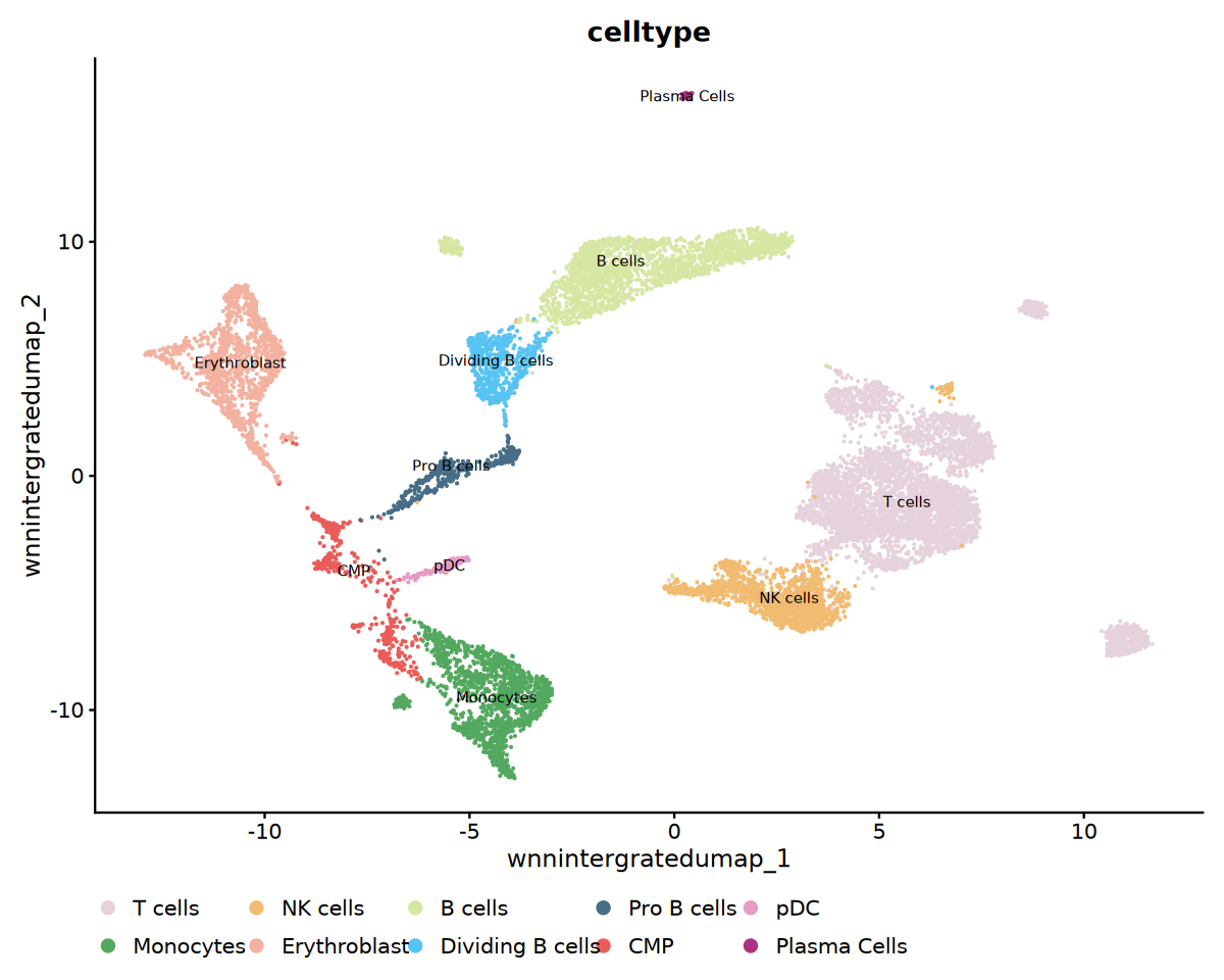

细胞类型注释结果分样本展开! 

10. Saving Results

saveRDS(obj_integrated, file = "integrated.rds")