ATAC + RNA Multi-omics: Co-variation Analysis of ATAC Accessible Regions and RNA Expression

Author: SeekGene

Time: 41 min

Words: 8.2k words

Updated: 2026-07-07

Reads: 0 times

1. Tutorial Overview

This tutorial is built on the Seurat and Signac frameworks and is designed to perform in-depth Peak-to-Gene association analysis on SeekArc single-cell multi-omics data (RNA + ATAC). By breaking through the limitations of linear distance and relying on the co-variation hypothesis, it reconstructs a high-resolution cis-regulatory network. This tutorial is intended for single-cell multi-omics data that have already undergone basic quality control, dimensionality reduction/clustering, and Peak Calling. Core analytical objectives include:

• Computing Peak–Gene Associations: Compute the co-variation between chromatin accessible regions (Peaks) and gene expression (RNA), identifying putative cis-regulatory relationships.
• Pseudobulk Construction: To improve the signal-to-noise ratio and robustness when computing correlations on single-cell data, construct pseudobulk matrices aggregated by cell subpopulation.
• Co-Regulatory Module K-means Clustering: Partition Peak–Gene association pairs with similar dynamic change patterns into distinct co-regulatory clusters.
• Joint Heatmap Visualization: Display ATAC accessibility Z-score and RNA expression Z-score side by side, intuitively presenting co-regulatory patterns across different cell populations.
• Transcription Factor Motif Enrichment Analysis: Perform TF Motif enrichment on the Peak sequences of each co-regulatory module, tracing back to upstream regulators.
• Target Gene GO/KEGG Functional Enrichment: Perform pathway enrichment on the target genes of each module, revealing the core biological functions engaged by the regulatory network.

Note

💡 The figures shown in the documentation represent only a subset of representative visualizations. For all complete analysis results (e.g., GO/KEGG/Motif enrichment results, etc.), please refer to the ./result/ directory.

suppressPackageStartupMessages(suppressWarnings({
    library(future)
    library(SeuratObject)
    library(Seurat)
    library(BiocGenerics)
    library(S4Vectors)
    library(IRanges)
    library(Signac)
    library(ComplexHeatmap)
    library(Biobase)
    library(AnnotationDbi)
    library(org.Hs.eg.db)
    #library(org.Mm.eg.db)
    library(JASPAR2020)
    library(TFBSTools)
    library(stringr)
    library(dplyr)
    library(DOSE)
    library(clusterProfiler)
    library(enrichplot)
    library(foreach)
    library(doParallel)
    library(base64enc) 
    library(KEGG.db)
}))

if (requireNamespace("future", quietly = TRUE)) {
    cores <- parallelly::availableCores()
    workers <- as.integer(floor(cores * 0.7))
    
    if (.Platform$OS.type == "unix") {
        future::plan(future::multicore, workers = workers)
    } else {
        future::plan(future::multisession, workers = workers)
    }
    
    message("total cores =", cores, "，uses ", workers, " works")
}

if (requireNamespace("memuse", quietly = TRUE)) {
    total_mem <- memuse::Sys.meminfo()$totalram
    total_mem_bytes <- as.numeric(total_mem)
    future_mem <- total_mem_bytes * 0.7
    future_mem_gb <- future_mem / 1024^3
    total_mem_gb <- total_mem_bytes / 1024^3
} else {
    future_mem <- 50 * 1024^3
    future_mem_gb <- 50
    total_mem_gb <- 50 / 0.6
}
options(future.globals.maxSize = future_mem)

2. Input File Preparation

2.1 Input File Requirements

This analysis tutorial performs Peak-to-Gene association analysis based on a pre-processed Seurat multi-omics object. Before starting, the following core input files need to be prepared:

• input.rds: The pre-processed Seurat object file. This object must contain both RNA and ATAC assays, and the ATAC modality must have already undergone basic Peak calling and Motif annotation.
• meta.tsv: Cell metadata file (tab-separated). Must contain the columns used to define cell types and sample groups, enabling subsequent extraction of cell subpopulations and clustering analyses as needed.
• genome.fa: Reference genome FASTA file for the corresponding species. Its main purpose is to extract the actual DNA sequences based on the genomic coordinates of ATAC peaks. Since downstream steps need to scan these sequences for the presence of specific transcription factor (TF) binding sites (Motifs), providing the exact reference genome sequence consistent with that used for single-cell alignment is a necessary prerequisite for Motif analysis.

2.2 Core Parameter Configuration

The following parameters control file paths, filtering thresholds, and analysis details. Please modify them according to your actual data:

# rds: Path to the input Seurat object RDS file; must contain pre-processed RNA and ATAC data.
rds = "/path/to/input.rds"

# meta: Path to the cell metadata file (TSV format), used to provide additional grouping or sample information. Leave empty if not needed.
meta = "/path/to/meta.tsv"

# genome_file: Path to the reference genome FASTA file for the corresponding species, used to extract sequences for Motif analysis.
genome_file = "/path/to/genome.fa"

# species: Species name ("human" or "mouse"), used to match the correct gene annotation library and TF database.
species = "human"

# clusters_col: Specifies which column in the metadata serves as the grouping basis for cell subpopulations (e.g., cell type).
clusters_col = "Celltype"

# celltypes: Comma-separated string specifying the names of cell subpopulations to include in the analysis.
celltypes = "B cells,CMP,Dividing B cells,Erythroblast,NK cells,pDC,Plasma Cells,Pro B cells,T cells"

# sample_col: Specifies which column in the metadata serves as the sample batch discriminator.
sample_col = "Sample"

# samples: Comma-separated string specifying the names of samples to include in the analysis.
samples = "XYRD_pbmc_2_arc,25030508_pbmc_1_arc"

# filter: Logical value string ("TRUE"/"FALSE"), whether to perform significance and variance filtering on Peak–Gene association pairs before clustering.
filter = "FALSE"

# corCutOff: Correlation score filtering threshold (absolute value). Only effective when filter is TRUE. Leave empty to indicate no restriction.
corCutOff = ""

# pCutOff: P-value significance filtering threshold. Only effective when filter is TRUE. Leave empty to indicate no restriction.
pCutOff = ""

# downsample: Logical value string ("True"/"False"), whether to randomly downsample each cell subpopulation before analysis to save memory.
downsample = "True"

# downsample_num: Downsample count — the maximum number of cells retained per cell subpopulation. Only effective when downsample is "True".
downsample_num = "1000"

# varCutOffATAC: Variance quantile threshold (0–1) for ATAC data. Filters out Peaks with extremely low variation. Only effective when filter is TRUE.
varCutOffATAC = ""

# varCutOffRNA: Variance quantile threshold (0–1) for RNA data. Filters out Genes with extremely stable expression. Only effective when filter is TRUE.
varCutOffRNA = ""

# k: Number of modules for K-means clustering, i.e., the expected number of clusters into which co-varying features are partitioned.
k = "10"

# nPlot: Maximum number of links randomly sampled for heatmap plotting, avoiding plot crashes caused by too many links.
nPlot = "1000"

outdir <- "./result"
dir.create(outdir, recursive = TRUE)

celltypes <- strsplit(celltypes,",")[[1]]
samples <- strsplit(samples,",")[[1]]

filter <- as.logical(filter)
corCutOff <- as.numeric(corCutOff)
pCutOff <- as.numeric(pCutOff)
varCutOffATAC <- as.numeric(varCutOffATAC)
varCutOffRNA <- as.numeric(varCutOffRNA)

k <- as.numeric(k)
nPlot <- as.numeric(nPlot)

3. Data Loading and Preprocessing

Once the environment, data, and parameters are all set up, begin loading and preprocessing the data for analysis.

3.1 Loading the Seurat Object and Metadata

Read the pre-processed multi-omics object and integrate additional cell classification information as needed.

obj <- readRDS(rds)
if (meta != ""){
  meta <- read.table(meta,header=T,sep='\t',check.names=F)
  rownames(meta) <- meta$barcode
  obj <- AddMetaData(obj, meta)
}
Idents(obj) <- obj@meta.data[[clusters_col]]

3.2 Cell Type Selection and Downsample Balancing

To reduce the memory footprint of the analysis and balance data volume across cell subpopulations, if the downsample mechanism is enabled, the object is first downsampled (limiting the maximum number of cells per subpopulation). Subsequently, the specified cell populations and samples are extracted according to the celltypes and samples parameters, and the factor levels of the cell subpopulations are rearranged in natural order.

if (exists("downsample") && downsample != "" && !is.na(as.logical(downsample)) && as.logical(downsample)) {
  if (exists("downsample_num") && downsample_num != "" && !is.na(as.numeric(downsample_num)) && as.numeric(downsample_num) > 1) {
    obj <- subset(obj, downsample = as.numeric(downsample_num))
  }
}

obj <- subset(obj, subset = !!sym(clusters_col) %in% celltypes)
obj <- subset(obj, subset = !!sym(sample_col) %in% samples)

v <- obj@meta.data[[clusters_col]]
sorted_levels <- stringr::str_sort(unique(as.character(v)), numeric = TRUE, na_last = TRUE)
obj@meta.data[[clusters_col]] <- factor(v, levels = sorted_levels, ordered = TRUE)

3.3 Reference Genome Processing

To prepare for downstream TF (transcription factor) analysis, the genome sequence file must first be processed: read genome.fa and convert it into a DNAStringSet object, while aligning the chromosome names of ATAC peaks in the object (retaining only shared chromosome information).

DefaultAssay(obj) <- "ATAC"
Idents(obj) <- clusters_col

library(Biostrings)
genome <- readDNAStringSet(genome_file)
names(genome) <- sub(" .*", "", names(genome)) 
keep_chromosomes <- unique(as.character(seqnames(granges(obj[["ATAC"]]))))
genome <- genome[which(names(genome) %in% keep_chromosomes)]
obj@assays$ATAC@ranges <- keepSeqlevels(granges(obj),keep_chromosomes, pruning.mode="coarse")

3.4 Motif Data Acquisition

Before performing transcription factor Motif enrichment analysis, we first need to obtain the reference Motif Position Frequency Matrix (PFM). Then use AddMotifs() to add Motif information to the ATAC Assay.

Why perform AddMotifs analysis in advance?

1. Building the Motif × Peak Matching Matrix: AddMotifs scans the ATAC Peak DNA sequences we just obtained, searching for transcription factor (TF) binding motifs (provided by pfm). This step globally stores the matching relationship between each Peak and Motif within the Seurat object.
2. Foundation for Downstream Module Enrichment: Subsequently, we cluster Peaks and Genes into multiple co-regulatory modules (Clusters). When it is time to perform Motif enrichment on the Peak set of a given module (to infer which TFs regulate these target genes), run_Motif_enrichment directly leverages the global matching information built here, without needing to re-scan sequences for each cluster — greatly improving computational efficiency.

species_tmp <- species
if (species_tmp == "human"){ 
     pfm <- getMatrixSet(x = JASPAR2020, opts = list(species = 9606, all_versions = TRUE)) 
     species = "hsa" 
     db = 'org.Hs.eg.db' 
     spe = "human" 
 } else if (species_tmp == "mouse"){ 
     pfm <- getMatrixSet(x = JASPAR2020, opts = list(species = 10090, all_versions = TRUE)) 
     species = "mmu" 
     db = 'org.Mm.eg.db' 
     spe = "mouse" 
 } else {
   stop("The value of 'species' is not supported.")
 }

obj <- AddMotifs(object = obj, genome = genome, pfm = pfm)

3.5 Definition of Core Helper Functions

Before entering the main analysis pipeline, we pre-define a series of core helper functions. These functions form the foundation for building advanced analysis pipelines, including:

• Logging and progress tracking (.ts_log)
• Metadata statistics and aggregation (.aggregate_meta)
• Wrapper for converting single-cell data to Pseudobulk objects (build_pseudobulk_seurat)
• K-means clustering algorithm for co-varying features (clusterRowsKmeans)
• Functional pathway enrichment analysis of downstream module genes (including go_enrich, kegg_enrich, run_Motif_enrichment)
• Integrated plotting and analysis engine (peak2GeneHeatmap)
• Basic network assessment and visualization statistical plot functions (plotPeaksPerGene, plotPeak2GeneVolcano, plotRankCorrelation)

1. .ts_log: Timestamped log output function. Its purpose is to add a standard time prefix to console output in long-running single-cell pipelines, enabling scholars to monitor analysis progress and locate time-consuming steps.

.ts_log <- function(...) {
  ts <- format(Sys.time(), "%Y-%m-%d %H:%M:%S")
  cat(sprintf("[%s] %s\n", ts, paste0(..., collapse = "")))
}

2. .majority_value: Mode statistics function. It primarily serves subsequent cell aggregation (Pseudobulk). When merging multiple cells into one pseudo-cell, numerical data can be averaged, but for character/factor data (e.g., cell-type names), we need to determine the most frequent category as the attribute of that pseudo-cell.

.majority_value <- function(x) {
  x <- x[!is.na(x)]
  if (length(x) == 0) return(NA)
  ux <- unique(x)
  ux[which.max(tabulate(match(x, ux)))]
}

3. .aggregate_meta: Metadata summarization function. Aggregates single-cell-level metadata by the specified grouping (e.g., Pseudobulk blocks): numerical columns are averaged, categorical columns take the mode — ensuring that the resulting pseudo-sample object still retains accurate annotation information after dimensionality reduction.

.aggregate_meta <- function(meta, groups) {
  stopifnot(length(groups) == nrow(meta))
  groups <- as.factor(groups)
  lv <- levels(groups)
  res_list <- lapply(lv, function(l) {
    idx <- which(groups == l)
    sub <- meta[idx, , drop = FALSE]
    out <- lapply(sub, function(col) {
      if (is.numeric(col) || is.integer(col)) {
        mean(col, na.rm = TRUE)
      } else if (is.logical(col)) {
        as.logical(.majority_value(col))
      } else if (is.factor(col)) {
        as.character(.majority_value(as.character(col)))
      } else if (inherits(col, "POSIXt") || inherits(col, "Date")) {
        suppressWarnings(mean(as.numeric(col), na.rm = TRUE))
      } else {
        .majority_value(as.character(col))
      }
    })
    out
  })
  df <- as.data.frame(do.call(rbind, res_list), stringsAsFactors = FALSE)
  rownames(df) <- lv
  df
}

4. build_pseudobulk_seurat: Main function for constructing Pseudobulk objects.
Single-cell data themselves are extremely sparse (with a large number of zeros). If Peak–Gene correlations are computed directly, the noise is overwhelming. The core purpose of this function is to aggregate and sum the Count values of multiple cells belonging to the same cell subpopulation (specified by the groupBy parameter), generating "super cells (Pseudobulk)." This not only effectively overcomes the Drop-out effect and improves the signal-to-noise ratio of expression and accessibility matrices, but also reduces matrix dimensionality by orders of magnitude, greatly accelerating the computational speed of subsequent analyses.

build_pseudobulk_seurat <- function(
  obj,
  groupBy,
  pseudobulkMem = 10,
  min_pseudobulk = 100,
  respect_group_boundaries = TRUE,
  keep_remainders = TRUE,
  seed = 1,
  verbose = TRUE
) {
  set.seed(seed)
  if (verbose) .ts_log("Start building pseudobulk (order_bin)")


  stopifnot("RNA" %in% names(obj@assays))
  stopifnot("ATAC" %in% names(obj@assays))

  meta <- obj@meta.data
  all_cells <- colnames(obj)


  rna_counts <- GetAssayData(obj, assay = "RNA", slot = "counts")
  atac_counts <- GetAssayData(obj, assay = "ATAC", slot = "counts")
  if (!inherits(rna_counts, "dgCMatrix")) rna_counts <- as(rna_counts, "dgCMatrix")
  if (!inherits(atac_counts, "dgCMatrix")) atac_counts <- as(atac_counts, "dgCMatrix")

  if (!(groupBy %in% colnames(meta))) {
    stop("Column not found in meta.data: ", groupBy)
  }

  cells_in_counts <- intersect(colnames(rna_counts), colnames(atac_counts))
  meta_sub <- meta[cells_in_counts, , drop = FALSE]
  if (verbose) .ts_log("Ordering by ", groupBy)
  ordered_cellID <- rownames(meta_sub[order(meta_sub[[groupBy]], na.last = NA), , drop = FALSE])


  x <- meta_sub[[groupBy]]
  uniq_n <- length(unique(x[!is.na(x)]))
  discrete_group <- is.factor(x) || is.character(x) || (is.numeric(x) && uniq_n <= max(50, ceiling(0.01 * length(x))))

  make_bins <- function(mem) {
    bins <- list()
    if (respect_group_boundaries && discrete_group) {
      if (verbose) .ts_log("Respecting group boundaries, ensuring no crossing of ", groupBy)

      grp_order <- unique(as.character(meta_sub[ordered_cellID, groupBy]))
      for (g in grp_order) {
        if (is.na(g)) next
        gi <- ordered_cellID[as.character(meta_sub[ordered_cellID, groupBy]) == g]
        if (length(gi) < mem && !keep_remainders) next
        n_bin_g <- if (keep_remainders) ceiling(length(gi) / mem) else floor(length(gi) / mem)
        if (n_bin_g > 0) {
          use_n <- (n_bin_g - 1) * mem
          if (n_bin_g > 1) {
            m <- matrix(gi[seq_len(use_n)], nrow = n_bin_g - 1, ncol = mem, byrow = TRUE)
            bins <- c(bins, split(m, row(m)))
          }

          if (keep_remainders) {
            rem <- gi[(use_n + 1):length(gi)]
            if (length(rem) > 0) bins <- c(bins, list(rem))
          } else if (length(gi) >= mem) {
            last_full <- gi[(use_n + 1):(use_n + mem)]
            bins <- c(bins, list(last_full))
          }
        }
      }
    } else {

      total_cells <- length(ordered_cellID)
      if (keep_remainders) {
        n_full <- floor(total_cells / mem)
        if (n_full > 0) {
          use_n <- n_full * mem
          m <- matrix(ordered_cellID[seq_len(use_n)], nrow = n_full, ncol = mem, byrow = TRUE)
          bins <- c(bins, split(m, row(m)))
        }
        if (total_cells > n_full * mem) {
          bins <- c(bins, list(ordered_cellID[(n_full * mem + 1):total_cells]))
        }
      } else {
        n_bin <- floor(total_cells / mem)
        if (n_bin > 0) {
          use_n <- n_bin * mem
          m <- matrix(ordered_cellID[seq_len(use_n)], nrow = n_bin, ncol = mem, byrow = TRUE)
          bins <- split(m, row(m))
        }
      }
    }
    bins
  }

  bins <- make_bins(pseudobulkMem)
  total_bins <- length(bins)
  if (total_bins < min_pseudobulk) {
    new_mem <- max(1, floor(length(ordered_cellID) / max(1, min_pseudobulk)))
    if (new_mem != pseudobulkMem) {
      if (verbose) .ts_log("Adjusting cells per pseudobulk to ", new_mem, " to meet minimum pseudobulk requirement")
      pseudobulkMem <- new_mem
      bins <- make_bins(pseudobulkMem)
      total_bins <- length(bins)
    }
  }
  if (total_bins < 1) stop("Insufficient cells to construct pseudobulks (group-boundary binning may have reduced availability)")

  selected <- as.character(unlist(bins, use.names = FALSE))
  pb_names <- paste0("pseudobulk", seq_len(total_bins))
  counts_per_bin <- vapply(bins, length, integer(1))
  pb_id <- factor(rep(pb_names, times = counts_per_bin), levels = pb_names)
  names(pb_id) <- selected

  if (verbose) {
    n_partial <- sum(counts_per_bin < pseudobulkMem)
    if (n_partial > 0) .ts_log(n_partial, " pseudobulks have fewer than ", pseudobulkMem, " cells")
  }


  selected <- intersect(selected, colnames(rna_counts))
  selected <- intersect(selected, colnames(atac_counts))
  if (length(selected) == 0) stop("No matching cells for aggregation")
  pb_id <- pb_id[selected]


  assign_mat <- Matrix::sparse.model.matrix(~ pb_id - 1)
  colnames(assign_mat) <- gsub("^pb_id", "", colnames(assign_mat))


  if (verbose) .ts_log("Aggregating RNA counts")
  rna_pb <- rna_counts[, selected, drop = FALSE] %*% assign_mat
  if (verbose) .ts_log("Aggregating ATAC counts")
  atac_pb <- atac_counts[, selected, drop = FALSE] %*% assign_mat
  colnames(rna_pb) <- colnames(atac_pb) <- colnames(assign_mat)


  if (verbose) .ts_log("Summarizing pseudobulk metadata")
  meta_sel <- meta[selected, , drop = FALSE]
  pb_meta <- .aggregate_meta(meta_sel, groups = pb_id)
  pb_meta$pb_id <- rownames(pb_meta)
  pb_meta$pb_index <- seq_len(nrow(pb_meta))

  pb_counts <- table(pb_id)
  pb_meta$pb_ncells <- as.integer(pb_counts[rownames(pb_meta)])
  if (groupBy %in% colnames(meta_sel)) {
    suppressWarnings(pb_meta[[paste0("mean_", groupBy)]] <- as.numeric(pb_meta[[groupBy]]))
  }

  pb_meta <- pb_meta[colnames(rna_pb), , drop = FALSE]

  pb_meta <- {
    .old <- pb_meta
    .new <- lapply(.old, function(col) {
      if (is.list(col)) {
        vapply(col, function(v) {
          if (length(v) == 0) return(NA_character_)
          paste(as.character(v), collapse = ";")
        }, character(1))
      } else if (is.numeric(col) || is.integer(col)) {
        col
      } else if (is.logical(col)) {
        as.character(col)
      } else {
        as.character(col)
      }
    })
    .df <- as.data.frame(.new, stringsAsFactors = FALSE)
    rownames(.df) <- rownames(.old)
    .df
  }

  if (groupBy %in% colnames(pb_meta)) {
    pb_meta[[groupBy]] <- as.character(pb_meta[[groupBy]])
  }

  # 4) ATAC annotation and genome information
  if (verbose) .ts_log("Preparing ATAC annotation and genome information")
  annotations <- tryCatch(Annotation(obj[["ATAC"]]), error = function(e) NULL)
  genome_info <- NULL
  if (!is.null(annotations) && inherits(obj[["ATAC"]], "ChromatinAssay")) {
    genome_info <- tryCatch({
      gi <- seqinfo(annotations)
      if (!is.null(gi)) gi@genome[1] else NA
    }, error = function(e) NA)
  }
  if (is.null(genome_info) || length(genome_info) == 0 || is.na(genome_info)) {
    genome_info <- tryCatch({ metadata(annotations)$genome }, error = function(e) NA)
  }
  if (is.null(genome_info) || length(genome_info) == 0 || is.na(genome_info)) {
    genome_info <- NULL
    if (verbose) .ts_log("Genome information not detected; leaving empty")
  }

  if (verbose) .ts_log("Building Seurat pseudobulk object (RNA) and running Normalize/Scale")
  pb_seurat <- CreateSeuratObject(counts = rna_pb, assay = "RNA", meta.data = pb_meta)

  md_existing <- pb_seurat@meta.data
  extra_cols <- setdiff(colnames(pb_meta), colnames(md_existing))
  if (length(extra_cols) > 0) {
    pb_seurat@meta.data <- cbind(
      md_existing,
      pb_meta[rownames(md_existing), extra_cols, drop = FALSE]
    )
  }

  try({ Idents(pb_seurat) <- pb_seurat$pb_id }, silent = TRUE)
  pb_seurat <- NormalizeData(pb_seurat, assay = "RNA")
  pb_seurat <- ScaleData(pb_seurat, assay = "RNA", features = rownames(pb_seurat[["RNA"]]))

  if (verbose) .ts_log("Adding ATAC assay and running TF-IDF/Scale")
  pb_seurat[["ATAC"]] <- CreateChromatinAssay(
    counts = atac_pb,
    annotation = annotations,
    genome = genome_info
  )
  DefaultAssay(pb_seurat) <- "ATAC"
  pb_seurat <- RunTFIDF(pb_seurat)
  pb_seurat <- ScaleData(pb_seurat, assay = "ATAC", features = rownames(pb_seurat[["ATAC"]]))

  if (verbose) .ts_log("Pseudobulk construction complete: columns = ", ncol(pb_seurat))

  mapping <- split(names(pb_id), f = as.character(pb_id))
  return(list(
    seurat = pb_seurat,
    mapping = mapping,
    meta = pb_meta
  ))
}

5. clusterRowsKmeans: K-means clustering algorithm wrapper. In Peak-to-Gene analysis, typically thousands of significantly co-varying Peak–Gene pairs are identified. The purpose of this function is to cluster features with similar cross-sample variation patterns (e.g., all up-regulated / highly accessible in a specific subpopulation) into the same class (co-regulatory module), based on the ATAC and RNA Z-score matrices. It not only performs clustering but also optimizes the returned Cluster ordering by hierarchically clustering the group means, resulting in a visually smoother module layout in the final heatmap.

clusterRowsKmeans <- function(atac_zscores, rna_zscores, cell_groups, k = 10, seed = 1) {
  set.seed(seed)
  m <- nrow(atac_zscores)
  if(k > m) {
    message(sprintf("Requested number of clusters (k=%d) exceeds number of data points (m=%d)", k, m))
    k <- 1
    message(sprintf("Automatically adjusting number of clusters to: k=%d", k))
  }

  k_clusters <- kmeans(atac_zscores, centers = k)
  cluster_ids <- k_clusters$cluster

  while(1 %in% table(cluster_ids)){
    k <- ceiling(k/2)
    message(sprintf("Too many clusters, automatically adjusting number of clusters to: k=%d", k))
    k_clusters <- kmeans(atac_zscores, centers = k)
    cluster_ids <- k_clusters$cluster
  }

  group_means_atac <- matrix(0, nrow = k, ncol = length(levels(as.factor(cell_groups))))
  colnames(group_means_atac) <- levels(as.factor(cell_groups))
  
  for (i in 1:k) {
    cluster_rows <- which(cluster_ids == i)
    if (length(cluster_rows) > 0) {
      cluster_atac <- atac_zscores[cluster_rows, , drop = FALSE]
      for (g in levels(as.factor(cell_groups))) {
        group_cells <- names(cell_groups)[cell_groups == g]
        if (length(group_cells) > 0) {
          group_means_atac[i, g] <- mean(rowMeans(cluster_atac[, group_cells, drop = FALSE]), na.rm = TRUE)
        }
      }
    }
  }

  hc <- hclust(dist(group_means_atac))
  cluster_order <- hc$order

  return(list(
    cluster_ids = cluster_ids,
    cluster_order = cluster_order,
    k = k
  ))
}

6. Functional Pathway Enrichment Analysis of Downstream Module Genes (go_enrich, kegg_enrich): After clustering features into multiple co-regulatory modules, understanding which biological functions each module (a set of related target genes) mainly participates in is crucial.

• go_enrich: Calls the clusterProfiler package to perform GO (Gene Ontology) enrichment analysis on module genes, automatically outputting bar plots, bubble plots, and detailed tabular data for annotation on the right side of the heatmap.
• kegg_enrich: Performs KEGG pathway enrichment analysis on module genes and outputs corresponding plots, revealing the enrichment status of metabolic or signaling pathways.

go_enrich <- function(eg,db,outdir,prefix) {
    if (is.null(eg) || nrow(eg) == 0) return(NULL)
    key_type <- if ("SYMBOL" %in% colnames(eg)) {
      "SYMBOL"
    } else if ("ENSEMBL" %in% colnames(eg)) {
      "ENSEMBL"
    } else if ("ENTREZID" %in% colnames(eg)) {
      "ENTREZID"
    } else {
      return(NULL)
    }
    genelist <- unique(as.character(eg[[key_type]]))
    genelist <- genelist[!is.na(genelist) & genelist != ""]
    if (length(genelist) == 0) return(NULL)
    go <- enrichGO(genelist, OrgDb=db, ont='ALL',pAdjustMethod = 'BH',qvalueCutoff = 1,pvalueCutoff = 1,keyType = key_type)
    go_df <- as.data.frame(go)
    if (is.null(go_df) || nrow(go_df) == 0) return(NULL)
    go1 <- data.frame(cluster=prefix, go_df)
    write.table(go1,file=paste(outdir,'/',prefix,'_GOenrich.xls',sep=''),sep='\t',quote=F,row.names=F)

    pdf(paste0(outdir,'/',prefix,'_GO_bar.pdf',sep=''),width = 10, height = 9)
    print(barplot(go,showCategory=20,drop=T)+ ggplot2::scale_y_discrete(labels = function(x) stringr::str_wrap(x, width = 50)))
    dev.off()
    pdf(paste0(outdir,'/',prefix,'_GO_dot.pdf',sep=''),width = 10, height = 8)
    print(dotplot(go,showCategory=20)+ ggplot2::scale_y_discrete(labels = function(x) stringr::str_wrap(x, width = 50)))
    dev.off()
    png(paste0(outdir,'/',prefix,'_GO_bar.png',sep=''),width = 780, height = 580)
    print(barplot(go,showCategory=20,drop=T)+ ggplot2::scale_y_discrete(labels = function(x) stringr::str_wrap(x, width = 50)))
    dev.off()
    png(paste0(outdir,'/',prefix,'_GO_dot.png',sep=''),width = 780, height = 580)
    print(dotplot(go,showCategory=20)+ ggplot2::scale_y_discrete(labels = function(x) stringr::str_wrap(x, width = 50)))
    dev.off()
    return(go1)
}

kegg_enrich <- function(eg, kegg_species, outdir, prefix) {
    if (is.null(eg) || nrow(eg) == 0) return(NULL)
    if (!("ENTREZID" %in% colnames(eg))) return(NULL)
    genenames <- if ("SYMBOL" %in% colnames(eg)) as.character(eg$SYMBOL) else as.character(eg$ENTREZID)
    names(genenames) <- as.character(eg$ENTREZID)
    genelist <- as.character(unique(eg$ENTREZID))
    internal_species_abbr <- c("hsa", "mmu", "rno", "gga", "ssc")
    if (species %in% internal_species_abbr) {
        use_internal <- TRUE
        kegg_species <- species
    } else {
        use_internal <- FALSE
        kegg_species <- species
    }
    kegg <- enrichKEGG(
        gene = genelist,
        organism = kegg_species,
        keyType = "kegg",
        pAdjustMethod = "BH",
        pvalueCutoff = 1,
        qvalueCutoff = 1,
        use_internal_data = use_internal
    )

    kegg_df <- as.data.frame(kegg)

    if (is.null(kegg_df) || nrow(kegg_df) == 0) {
        message(sprintf("[跳过] %s: KEGG无显著条目", prefix))
        return(NULL)
    }

    gene_list <- strsplit(as.character(kegg_df$geneID), split = "/")
    geneName <- vapply(
        gene_list,
        function(x) paste(genenames[x], collapse = "/"),
        character(1)
    )

    kegg_df$Description <- sub("\\s+-\\s+[^\\(]+\\s*\\([^)]+\\)\\s*$", "",as.character(kegg_df$Description))

    KEGGenrich <- data.frame(
        cluster = prefix,
        kegg_df,
        geneName = geneName,
        stringsAsFactors = FALSE
    )

    write.table(
        KEGGenrich,
        file = paste0(outdir, "/", prefix, "_KEGGenrich.xls"),
        sep = "\t",
        quote = FALSE,
        row.names = FALSE
    )

    pdf(paste0(outdir, "/", prefix, "_KEGG_dot.pdf"), width = 8, height = 8)
    print(dotplot(kegg, showCategory = 20) +
              ggplot2::scale_y_discrete(labels = function(x) stringr::str_wrap(x, width = 50)))
    dev.off()

    pdf(paste0(outdir, "/", prefix, "_KEGG_bar.pdf"), width = 8, height = 8)
    print(barplot(kegg, showCategory = 20) +
              ggplot2::scale_y_discrete(labels = function(x) stringr::str_wrap(x, width = 50)))
    dev.off()

    png(paste0(outdir, "/", prefix, "_KEGG_dot.png"), width = 780, height = 580)
    print(dotplot(kegg, showCategory = 20) +
              ggplot2::scale_y_discrete(labels = function(x) stringr::str_wrap(x, width = 50)))
    dev.off()

    png(paste0(outdir, "/", prefix, "_KEGG_bar.png"), width = 780, height = 580)
    print(barplot(kegg, showCategory = 20) +
              ggplot2::scale_y_discrete(labels = function(x) stringr::str_wrap(x, width = 50)))
    dev.off()
    return(KEGGenrich)
}

7. run_Motif_enrichment: Motif enrichment function for module Peak sequences. For each cluster, we extract the set of Peaks it contains and call Signac::FindMotifs to perform a hypergeometric test. The purpose of this function is to answer: "Among these chromatin accessible regions with similar dynamic changes, which transcription factors' binding sites are significantly enriched?" The results will serve as the core annotation on the left side of the heatmap.

run_Motif_enrichment <- function(obj, peaks) {
  if (is.null(Signac::Motifs(obj[["ATAC"]])) || length(peaks) == 0) return(NULL)
  tryCatch({
    motif_res <- Signac::FindMotifs(
      object = obj,
      assay = "ATAC",
      features = peaks
    )
    if (!is.null(motif_res) && nrow(motif_res) > 0) {
      return(as.data.frame(motif_res))
    }
  }, error = function(e) { 
    message("Motif Error: ", e$message)
    NULL 
  })
  return(NULL)
}

8. peak2GeneHeatmap: Integrated plotting and analysis engine for the Peak-to-Gene analysis pipeline. This substantial function is the core executor of this script. Its purpose is:

1. Receive the results of Signac::Links and the Pseudobulk object.
2. Filter low-confidence connections based on user parameters.
3. Convert the filtered ATAC and RNA data into standardized Z-score matrices.
4. Call clusterRowsKmeans for co-regulatory module clustering.
5. For each Cluster, automatically call enrichment functions (Motif, GO, KEGG) and save the result tables.
6. Use the ComplexHeatmap package to construct heatmap objects for dual-omics data, clustering results, and enrichment text annotations, and return the heatmap object for external rendering of a publication-quality high-resolution panoramic heatmap.

peak2GeneHeatmap <- function( 
   seurat_obj, 
   links, 
   filter = FALSE, 
   corCutOff = 0.45, 
   pCutOff = 0.0001, 
   varCutOffATAC = 0.25, 
   varCutOffRNA = 0.25, 
   k = 10, 
   nPlot = 5000, 
   groupBy = "seurat_clusters", 
   palGroup = NULL, 
   palATAC = ArchR::paletteContinuous("solarExtra"), 
   palRNA = ArchR::paletteContinuous("blueYellow"), 
   seed = 1, 
   run_enrichment = TRUE 
 ) { 
   set.seed(seed) 
   
   peak_matrix <- GetAssayData(seurat_obj, assay = "ATAC", slot = "data") 
   peak_vars <- MatrixGenerics::rowVars(peak_matrix) 
   peak_var_quantiles <- rank(peak_vars) / length(peak_vars) 
   names(peak_var_quantiles) <- rownames(peak_matrix) 
   
   rna_matrix <- GetAssayData(seurat_obj, assay = "RNA", slot = "data") 
   rna_vars <- MatrixGenerics::rowVars(rna_matrix) 
   rna_var_quantiles <- rank(rna_vars) / length(rna_vars) 
   names(rna_var_quantiles) <- rownames(rna_matrix) 
 
   links_data <- data.frame( 
     peak = links$peak, gene = links$gene, score = links$score, pvalue = links$pvalue 
   ) 
   links_data <- subset(links_data, !is.na(peak) & !is.na(gene) & !is.na(score) & !is.na(pvalue)) 
   
   if (filter){ 
     links_filtered <- links_data[abs(links_data$score) >= corCutOff & links_data$pvalue <= pCutOff, ] 
     links_filtered$peak_id <- match(links_filtered$peak, rownames(peak_matrix)) 
     links_filtered$gene_id <- match(links_filtered$gene, rownames(rna_matrix)) 
     links_filtered$VarQATAC <- peak_var_quantiles[rownames(peak_matrix)[links_filtered$peak_id]] 
     links_filtered$VarQRNA <- rna_var_quantiles[rownames(rna_matrix)[links_filtered$gene_id]] 
     links_filtered <- links_filtered[links_filtered$VarQATAC > varCutOffATAC, ] 
     links_filtered <- links_filtered[links_filtered$VarQRNA > varCutOffRNA, ] 
   } else { 
     links_filtered <- links_data 

     links_filtered$peak_id <- match(links_filtered$peak, rownames(peak_matrix)) 
     links_filtered$gene_id <- match(links_filtered$gene, rownames(rna_matrix)) 
     
     links_filtered$VarATAC <- peak_vars[links_filtered$peak_id] 
     links_filtered$VarRNA <- rna_vars[links_filtered$gene_id] 
     
     links_filtered <- links_filtered[links_filtered$VarATAC > 0 & links_filtered$VarRNA > 0, ] 
     

     links_filtered$VarATAC <- NULL 
     links_filtered$VarRNA <- NULL 
   } 
 
   if (nrow(links_filtered) == 0) stop("is NA") 
 
   peak_ids <- match(links_filtered$peak, rownames(peak_matrix)) 
   gene_ids <- match(links_filtered$gene, rownames(rna_matrix)) 
   
   atac_data <- peak_matrix[peak_ids, ] 
   rna_data <- rna_matrix[gene_ids, ] 
   
   rowZscores <- function(matrix1, matrix2, min = NULL, max = NULL, limit = TRUE) { 
     z1 <- t(scale(t(matrix1))) 
     z2 <- t(scale(t(matrix2))) 
     if(limit) { 
         if(is.null(min) || is.null(max)) { 
           middle_range1 <- quantile(abs(z1), probs = 0.875, na.rm = TRUE) 
           if (middle_range1 < 1) { min1 <- -1; max1 <- 1 
           } else if (middle_range1 < 1.5) { min1 <- -1.5; max1 <- 1.5 
           } else { min1 <- -2; max1 <- 2 } 
           
           middle_range2 <- quantile(abs(z2), probs = 0.875, na.rm = TRUE) 
           if (middle_range2 < 1) { min2 <- -1; max2 <- 1 
           } else if (middle_range2 < 1.5) { min2 <- -1.5; max2 <- 1.5 
           } else { min2 <- -2; max2 <- 2 } 
           
           min <- max(min1, min2) 
           max <- min(max1, max2) 
         } 
         z1[z1 > max] <- max; z1[z1 < min] <- min 
         z2[z2 > max] <- max; z2[z2 < min] <- min 
     } 
     return(list(matrix1 = z1, matrix2 = z2)) 
   } 
 
   zs <- rowZscores(as.matrix(atac_data), as.matrix(rna_data)) 
   atac_zscores <- zs$matrix1 
   rna_zscores <- zs$matrix2 
 
   cell_groups <- seurat_obj@meta.data[, groupBy] 
   names(cell_groups) <- colnames(seurat_obj) 
   v <- seurat_obj@meta.data[[groupBy]] 
   sorted_levels <- stringr::str_sort(unique(as.character(v)), numeric = TRUE, na_last = TRUE) 
   cell_groups <- factor(v, levels = sorted_levels, ordered = TRUE) 
   
   clust_res <- clusterRowsKmeans(atac_zscores, rna_zscores, cell_groups, k = k, seed = seed) 
   cluster_ids <- clust_res$cluster_ids 
   cluster_order <- clust_res$cluster_order 
   k <- clust_res$k 
 
   ordered_links <- list() 
   ordered_atac <- list() 
   ordered_rna <- list() 
   cluster_info_list <- list() 
    
   row_split_factor <- c() 
   
   for (i in seq_along(cluster_order)) { 
     orig_cluster_id <- cluster_order[i] 
     cluster_rows <- which(cluster_ids == orig_cluster_id) 
     if (length(cluster_rows) > 0) { 
       ordered_links <- c(ordered_links, list(links_filtered[cluster_rows, ])) 
       ordered_atac <- c(ordered_atac, list(atac_zscores[cluster_rows, ])) 
       ordered_rna <- c(ordered_rna, list(rna_zscores[cluster_rows, ])) 
       
       cluster_links <- links_filtered[cluster_rows, ] 
       cluster_links$kmeans_cluster <- i 
       cluster_info_list[[i]] <- cluster_links 
       
       row_split_factor <- c(row_split_factor, rep(i, length(cluster_rows))) 
     } 
   } 
   
   ordered_links_df <- do.call(rbind, ordered_links) 
   ordered_atac_mat <- do.call(rbind, ordered_atac) 
   ordered_rna_mat <- do.call(rbind, ordered_rna) 
   cluster_info_df <- do.call(rbind, cluster_info_list) 
 
   write.table(cluster_info_df, file = file.path(dirname(outdir), "result", "Peak2Gene_Kmeans_Clusters.tsv"), 
               sep = "\t", row.names = FALSE, col.names = TRUE, quote = FALSE) 
 
   atac_row_anno_text <- rep("", k) 
   rna_row_anno_text <- rep("", k) 
   
   if (run_enrichment) { 
     enrich_outdir <- file.path(dirname(outdir), "result", "Cluster_Enrichment") 
     dir.create(enrich_outdir, showWarnings = FALSE, recursive = TRUE) 
     has_motif <- !is.null(Signac::Motifs(obj[["ATAC"]])) 
    if (!has_motif) { 
      .ts_log("ATAC assay has no Motifs") 
    } 
    
    all_motif_res <- list()
    all_go_res <- list()
    all_kegg_res <- list()
    for (cid in seq_len(k)) { 
      sub_df <- cluster_info_df[cluster_info_df$kmeans_cluster == cid, ] 
      if(nrow(sub_df) == 0) next 
      
      .ts_log(cid) 
      
      motif_res <- run_Motif_enrichment(obj, unique(sub_df$peak)) 
      if (!is.null(motif_res)) { 
        motif_res$cluster <- as.character(cid)
        all_motif_res[[as.character(cid)]] <- motif_res
        write.table(motif_res, file.path(enrich_outdir, paste0("Cluster_", cid, "_Motif.tsv")), sep="\t", row.names=F, quote=F) 
         top6_motif <- head(motif_res[order(motif_res$pvalue), "motif.name"], 6) 
         top6_motif <- gsub("\\s*\\(.*\\)", "", top6_motif)  
           
         if(length(top6_motif) > 0) { 
           line1 <- paste(top6_motif[seq_len(min(3, length(top6_motif)))], collapse = "  ") 
           line2 <- if (length(top6_motif) > 3) paste(top6_motif[4:min(6, length(top6_motif))], collapse = "  ") else NULL 
           atac_row_anno_text[cid] <- paste(c(line1, line2), collapse = "\n") 
         } 
       } else { 
         .ts_log("Cluster ", cid, " no Motif") 
       } 
       
       genes_raw <- unique(as.character(sub_df$gene)) 
       genes_raw <- genes_raw[!is.na(genes_raw) & genes_raw != ""] 
       genes_clean <- genes_raw 
       .ts_log("Cluster ", cid, " number: ", length(genes_clean)) 
       
       eg <- NULL 
       used_from <- "SYMBOL" 
       
       eg_try <- tryCatch({ 
         clusterProfiler::bitr( 
           genes_clean, 
           fromType = used_from, 
           toType = unique(c("SYMBOL", "ENSEMBL", "ENTREZID")), 
           OrgDb = get(db) 
         ) 
       }, error = function(e) NULL) 
       
       if (!is.null(eg_try) && nrow(eg_try) > 0) { 
         eg <- unique(eg_try) 
       } 
 
       if (!is.null(eg) && nrow(eg) > 0) { 
         keep_cols <- intersect(c("SYMBOL", "ENSEMBL", "ENTREZID"), colnames(eg)) 
         eg <- unique(eg[, keep_cols, drop = FALSE]) 
         .ts_log("Cluster ", cid, " suscuss: ", nrow(eg), "fromType=", used_from) 
       } else { 
         .ts_log("Cluster ", cid, " failure") 
       } 
 
       go_res <- go_enrich( 
         eg = eg, 
         db = get(db), 
         outdir = enrich_outdir, 
         prefix = paste0("Cluster_", cid) 
       ) 
       if (!is.null(go_res)) { 
         go_res_df <- as.data.frame(go_res)
         if (nrow(go_res_df) > 0) {
           go_res_df$cluster <- as.character(cid)
           all_go_res[[as.character(cid)]] <- go_res_df
         }
         
         top5_go <- head(go_res_df[order(go_res_df$p.adjust), "Description"], 5) 
         if (length(top5_go) > 0) { 
           go_text <- stringr::str_wrap(paste(top5_go, collapse = "; "), width = 100) 
           go_lines <- strsplit(go_text, "\n", fixed = TRUE)[[1]] 
           rna_row_anno_text[cid] <- paste(head(go_lines, 2), collapse = "\n") 
         } 
       } else { 
         .ts_log("Cluster ", cid, " no GO Term") 
       } 
       
        kegg_res <- tryCatch({ 
          kegg_enrich( 
            eg = eg, 
            kegg_species = kegg_species, 
            outdir = enrich_outdir, 
            prefix = paste0("Cluster_", cid) 
          ) 
        }, error = function(e) { 
          .ts_log("Cluster ", cid, " KEGG", e$message) 
          return(NULL) 
        }) 
        
        if (!is.null(kegg_res)) { 
          kegg_res_df <- as.data.frame(kegg_res)
          if (nrow(kegg_res_df) > 0) {
            kegg_res_df$cluster <- as.character(cid)
            all_kegg_res[[as.character(cid)]] <- kegg_res_df
        } else { 
          .ts_log("Cluster ", cid, " no KEGG Pathway") 
        } 
     } 
     if (length(all_motif_res) > 0) {
       combined_motif <- do.call(rbind, all_motif_res)
       write.table(combined_motif, file.path(enrich_outdir, "All_Cluster_Motif.tsv"), sep="\t", row.names=F, quote=F)
     }
     
     if (length(all_go_res) > 0) {
       combined_go <- do.call(rbind, all_go_res)
       write.table(combined_go, file.path(enrich_outdir, "All_Cluster_GOenrich.xls"), sep="\t", row.names=F, quote=F)
       .ts_log("Saved in All_Cluster_GOenrich.xls。")
     }
     
     if (length(all_kegg_res) > 0) {
       combined_kegg <- do.call(rbind, all_kegg_res)
       write.table(combined_kegg, file.path(enrich_outdir, "All_Cluster_KEGGenrich.xls"), sep="\t", row.names=F, quote=F)
       .ts_log("Saved in All_Cluster_KEGGenrich.xls。")
     }
   } 
 
   if(nrow(cluster_info_df) < 20) stop("Too few links") 
   plot_idx <- seq_len(nrow(cluster_info_df)) 
   if (nrow(cluster_info_df) > nPlot) { 

     plot_idx <- sort(sample(plot_idx, nPlot)) 
   } 
   links_filtered <- ordered_links_df[plot_idx, , drop = FALSE] 
   ordered_atac_mat <- ordered_atac_mat[plot_idx, , drop = FALSE] 
   ordered_rna_mat <- ordered_rna_mat[plot_idx, , drop = FALSE] 

   row_split_factor <- row_split_factor[plot_idx] 
 
   if (is.null(palGroup)) { 
     group_levels <- levels(as.factor(cell_groups)) 
     palGroup <- setNames(scales::hue_pal()(length(group_levels)), group_levels) 
   } 
   
   n_groups <- length(unique(cell_groups)) 
   legend_nrow <- ifelse(n_groups > 8, ceiling(n_groups / 8), 1) 
 
   column_atac <- ComplexHeatmap::HeatmapAnnotation(Group = cell_groups, col = list(Group = palGroup), show_legend = FALSE, show_annotation_name = FALSE) 
   column_rna <- ComplexHeatmap::HeatmapAnnotation( 
     Cell = cell_groups, 
     col = list(Cell = palGroup), 
     show_annotation_name = FALSE, 
     annotation_legend_param = list( 
       Cell = list(nrow = legend_nrow, title_position = "topcenter")
     ) 
   ) 
 
   split_fac <- factor(row_split_factor, levels = seq_len(k)) 
   
   cluster_mid_row <- vapply(seq_len(k), function(cid) { 
     idx <- which(split_fac == cid) 
     if (length(idx) == 0) NA_integer_ else as.integer(round(mean(range(idx)))) 
   }, integer(1)) 
   

   valid_cid_atac <- which(!is.na(cluster_mid_row) & nzchar(atac_row_anno_text)) 
   mark_at_atac <- cluster_mid_row[valid_cid_atac] 
   mark_labels_atac <- atac_row_anno_text[valid_cid_atac] 
 
   row_anno_atac <- ComplexHeatmap::rowAnnotation( 
     Motif = ComplexHeatmap::anno_mark( 
       at = mark_at_atac, 
       labels = mark_labels_atac, 
       which = "row", 
       side = "left",
       labels_gp = grid::gpar(fontsize = 10, fontface = "bold", col = "#0c0c0cff"), 
       lines_gp = grid::gpar(lty = 2, col = "black"), 
       link_width = unit(5, "mm"), 
       padding = unit(1.5, "mm"), 
       extend = unit(c(1, 10), "mm") 
     ), 
     width = unit(1, "cm") 
   ) 
   
   valid_cid_rna <- which(!is.na(cluster_mid_row) & nzchar(rna_row_anno_text)) 
   mark_at_rna <- cluster_mid_row[valid_cid_rna] 
   mark_labels_rna <- stringr::str_wrap(rna_row_anno_text[valid_cid_rna], width = 65) 
   
   row_anno_rna <- ComplexHeatmap::rowAnnotation( 
     GO = ComplexHeatmap::anno_mark( 
       at = mark_at_rna, 
       labels = mark_labels_rna, 
       which = "row", 
       side = "right",
       labels_gp = grid::gpar(fontsize = 10, fontface = "bold", col = "#0c0c0cff"), 
       lines_gp = grid::gpar(lty = 2, col = "black"), 
       link_width = unit(8, "mm"), 
       padding = unit(0.005, "mm"), 
       extend = unit(c(0.001, 1), "mm") 
     ), 
     width = unit(1, "cm") 
   ) 
   
   panel_width <- unit(max(10, ncol(ordered_rna_mat) * 0.02), "cm") 
 
   atac_heatmap <- ComplexHeatmap::Heatmap( 
     ordered_atac_mat, 
     name = "ATAC Z-score", 
     col = palATAC, 
     cluster_rows = FALSE, cluster_columns = FALSE, 
     column_order = order(colMeans(ordered_rna_mat), decreasing = TRUE), 
     show_row_names = FALSE, show_column_names = FALSE, 
     top_annotation = column_atac, 
     left_annotation = row_anno_atac,  
     column_split = cell_groups, column_gap = unit(0, "mm"), column_title = NULL, 
     
     row_order = seq_len(nrow(ordered_atac_mat)), 
     cluster_row_slices = FALSE, 
     width = panel_width, 
     use_raster = TRUE, raster_quality = 1, 
     heatmap_legend_param = list(direction = "horizontal", title_position = "topcenter") 
   ) 
   
   rna_heatmap <- ComplexHeatmap::Heatmap( 
     ordered_rna_mat, 
     name = "RNA Z-score", 
     col = palRNA, 
     cluster_rows = FALSE, cluster_columns = FALSE, 
     column_order = order(colMeans(ordered_rna_mat), decreasing = TRUE), 
     show_row_names = FALSE, show_column_names = FALSE, 
     top_annotation = column_rna, 
     right_annotation = row_anno_rna, 
     column_split = cell_groups, column_gap = unit(0, "mm"), column_title = NULL, 
     
     width = panel_width, 
     use_raster = TRUE, raster_quality = 1, 
     heatmap_legend_param = list(direction = "horizontal", title_position = "topcenter") 
   ) 
 
   return(list(
     links = cluster_info_df,
     atac_heatmap = atac_heatmap, 
     rna_heatmap = rna_heatmap
   )) 
 }
}

9. plotPeaksPerGene: Basic statistical plot function (gene regulatory-degree distribution). A gene may be co-regulated by multiple surrounding Enhancers (Peaks). This function plots a histogram, intuitively displaying "on average, how many Peaks are associated with each gene" in the global network — helping to evaluate the complexity and connectivity of the regulatory network.

plotPeaksPerGene <- function(links) {
  gene_counts <- table(links$gene)
  gene_counts_df <- data.frame(
    gene = names(gene_counts),
    count = as.numeric(gene_counts)
  )
    
  median_linked_Peaks <- median(gene_counts_df$count)
  
  p <- ggplot2::ggplot(gene_counts_df, ggplot2::aes(x = count)) +
    ggplot2::geom_histogram(binwidth = 1, fill = "black", color = "white") +
    ggplot2::geom_vline(xintercept = median_linked_Peaks, linetype = "dashed", color = "gray") +
    ggplot2::annotate("text", x = 10, y = 1000, 
             label = paste0("Median Linked Peaks = ", median_linked_Peaks)) +
    ggplot2::labs(x = "Number of linked peaks", y = "Number of genes") +
    ggplot2::theme_classic() +
    ggplot2::xlim(0, 25)
    
  return(p)
}

10. plotPeak2GeneVolcano: Basic statistical plot function (association significance volcano plot). Similar to the volcano plot in differential expression analysis, this displays the Correlation (X-axis) and P-value (Y-axis) for all Peak–Gene pairs. It helps scholars identify at a glance the "Top core driver genes" that have both extremely strong correlation and extremely high statistical significance.

plotPeak2GeneVolcano <- function(links, topN = 20, p = 0.05, score = 0.05) {
  volcano_data <- data.frame(
    peak = links$peak,
    gene = links$gene,
    correlation = links$score,
    pvalue = links$pvalue,
    logPvalue = -log10(links$pvalue + 1e-300)
  )
  
  top_genes_indices <- order(volcano_data$logPvalue, decreasing = TRUE)[1:min(topN, nrow(volcano_data))]
  top_genes <- volcano_data[top_genes_indices, ]
  
  volcano_data$highlighted <- "No"
  volcano_data$highlighted[top_genes_indices] <- "Yes"
  top_genes$highlighted <- "Yes"
  
  p <- ggplot2::ggplot(volcano_data, ggplot2::aes(x = correlation, y = logPvalue, color = highlighted)) +
    ggplot2::geom_point(alpha = 0.6, size = 1) +
    ggplot2::scale_color_manual(values = c("No" = "gray", "Yes" = "red")) +
    ggplot2::labs(
      # title = "Peak-to-Gene Linkage Volcano Plot",
      x = "Correlation Score",
      y = "-log10(p-value)",
      color = "Top Genes"
    ) +
    ggplot2::theme_classic() +
    ggplot2::theme(
      legend.position = "none",
      # text = element_text(family = "sans")
    ) +
    ggplot2::geom_vline(xintercept = -score, linetype = "dashed", color = "black", alpha = 0.7) +
    ggplot2::geom_vline(xintercept = score, linetype = "dashed", color = "black", alpha = 0.7) +
    ggplot2::geom_hline(yintercept = -log10(p), linetype = "dashed", color = "black", alpha = 0.7) 
  
  if(nrow(top_genes) > 0) {
    p <- p + ggrepel::geom_text_repel(
      data = top_genes,
      # family = "sans",
      ggplot2::aes(label = gene),
      size = 3,
      box.padding = 0.5,
      point.padding = 0.2,
      force = 2,
      max.overlaps = 20
    )
  }
  
  return(p)
}

11. plotRankCorrelation: Basic statistical plot function (correlation rank plot). Rank all association pairs by correlation coefficient from largest to smallest and plot the curve. This can be used to evaluate the proportional distribution trend of strong versus weak correlation pairs in the overall network.

plotRankCorrelation <- function(links) {
  all_correlations <- links$score
  
  sorted_correlations <- sort(all_correlations, decreasing = TRUE)
  correlation_df <- data.frame(
    rank = 1:length(sorted_correlations),
    correlation = sorted_correlations
  )
  p <- ggplot2::ggplot(correlation_df, ggplot2::aes(x = rank, y = correlation)) +
    ggplot2::geom_line(linewidth = 1) +
    ggplot2::geom_hline(yintercept = 0, linetype = "solid", color = "black") +
    ggplot2::labs(
      # title = "Peak-Gene correlation",
      x = "Peak-Gene Linkage",
      y = "Correlation Score"
    ) +
    ggplot2::theme_classic() +
    ggplot2::theme(
      # text = element_text(family = "sans"),
      axis.title = ggplot2::element_text(size = 14),
      axis.text = ggplot2::element_text(size = 12),
      plot.title = ggplot2::element_text(hjust = 0.5, size = 14),
      axis.text.x = ggplot2::element_blank(),
      axis.ticks.x = ggplot2::element_blank()
    )
  
  return(p)
}

4. Peak-to-Gene Association

Peak-to-Gene analysis is the core step of this tutorial. Since regulatory elements such as Enhancers may regulate target gene expression over long linear distances via chromatin spatial folding, relying solely on linear distance (e.g., promoter regions) often fails to accurately capture such regulatory relationships. Here, we first check whether the object already contains association information; if not, we first compute regional statistics such as GC content (RegionStats), then use the LinkPeaks function provided by Signac to compute the statistical co-variation (Correlation) between each chromatin-accessible Peak and the expression level of nearby genes. If, within the same cell, changes in a Peak's accessibility are consistently accompanied by synchronous changes in a specific gene's expression, we can hypothesize that a cis-regulatory relationship exists between them.

invisible(capture.output({
  suppressMessages(suppressWarnings({ 
    links_all <- Signac::Links(obj[["ATAC"]]) 
    
    if (length(links_all) == 0) { 
    
      obj <- RegionStats( 
        object = obj, 
        genome = genome, 
        assay = "ATAC" 
      ) 
      
      obj <- LinkPeaks( 
          object = obj, 
          peak.assay = "ATAC", 
          expression.assay = "RNA" 
      ) 
      
      links_all <- Signac::Links(obj[["ATAC"]]) 
      
      if (length(links_all) == 0) { 
        stop("no peak-to-gene links") 
      } 
    } 
    
    write.table( 
      as.data.frame(links_all), 
      file = file.path(outdir, "Gene2PeakLinks.xls"), 
      sep = "\t", 
      row.names = FALSE, 
      col.names = TRUE, 
      quote = FALSE 
    )          
  }))
}))

saveRDS(obj, file.path(outdir, "output.rds"))

5. Constructing the Pseudobulk Matrix

After obtaining the basic Peak-to-Gene links, directly using the sparse single-cell matrix to compute fine-grained dynamic differences between groups (e.g., across Clusters) is often severely confounded by Drop-out (loss of sequencing signal). To improve the signal-to-noise ratio, enhance the robustness of correlation computation, and substantially reduce the computational cost of downstream clustering heatmaps, we use the build_pseudobulk_seurat function to sum (aggregate) the Count matrices of hundreds of cells belonging to the same group, according to the cell group identifier (clusters_col), producing a low-dimensional, high-SNR Pseudobulk object.

invisible(capture.output({
  suppressMessages(suppressWarnings({ 
    res <- build_pseudobulk_seurat(obj = obj, groupBy = clusters_col) 
    pseudo_obj <- res$seurat 
  }))
}))

6. Co-Regulatory Module K-means Clustering and Enrichment Analysis

This is the most complex and critical data integration and visualization step in the pipeline, automatically completed by our wrapped peak2GeneHeatmap function. It implements the following complete pipeline:

1. Data Filtering and Scaling: Filter out low-confidence association pairs based on set thresholds (corCutOff, pCutOff), and convert the expression and accessibility data in the Pseudobulk matrix into standardized Z-score matrices.
2. K-means Module Clustering: Partition Peak–Gene combinations with similar dynamic change trends (i.e., simultaneously up- or down-regulated in the same cell populations) into k distinct co-regulatory clusters.
3. Functional Enrichment Inference:
   • Upstream Regulatory Tracing (Motif): Perform transcription factor Motif enrichment analysis on the Peak sequences of each cluster, inferring which TFs drive the accessibility of that module.
   • Downstream Function Elucidation (GO/KEGG): Perform pathway enrichment on the target genes associated with each cluster, explaining which biological processes these genes mainly participate in.
4. Joint Heatmap Object Construction: Use ComplexHeatmap to construct heatmap objects for ATAC signal, RNA signal, Motif annotation (left), GO annotation (right), and return them for external rendering as an intuitive multi-omics regulatory network panoramic view.

result <- peak2GeneHeatmap( 
      pseudo_obj, 
      links = links_all, 
      filter = filter, 
      corCutOff = corCutOff, 
      pCutOff = pCutOff, 
      varCutOffATAC = varCutOffATAC, 
      varCutOffRNA = varCutOffRNA, 
      k = k, 
      nPlot = nPlot, 
      groupBy = clusters_col 
)

options(repr.plot.width = 20, repr.plot.height = 10)
draw((result$atac_heatmap + result$rna_heatmap), 
     heatmap_legend_side = "bottom", 
     annotation_legend_side = "bottom", 
     ht_gap = unit(1, "mm"), 
     auto_adjust = TRUE,
     padding = unit(c(4, 3, 20, 15), "mm"))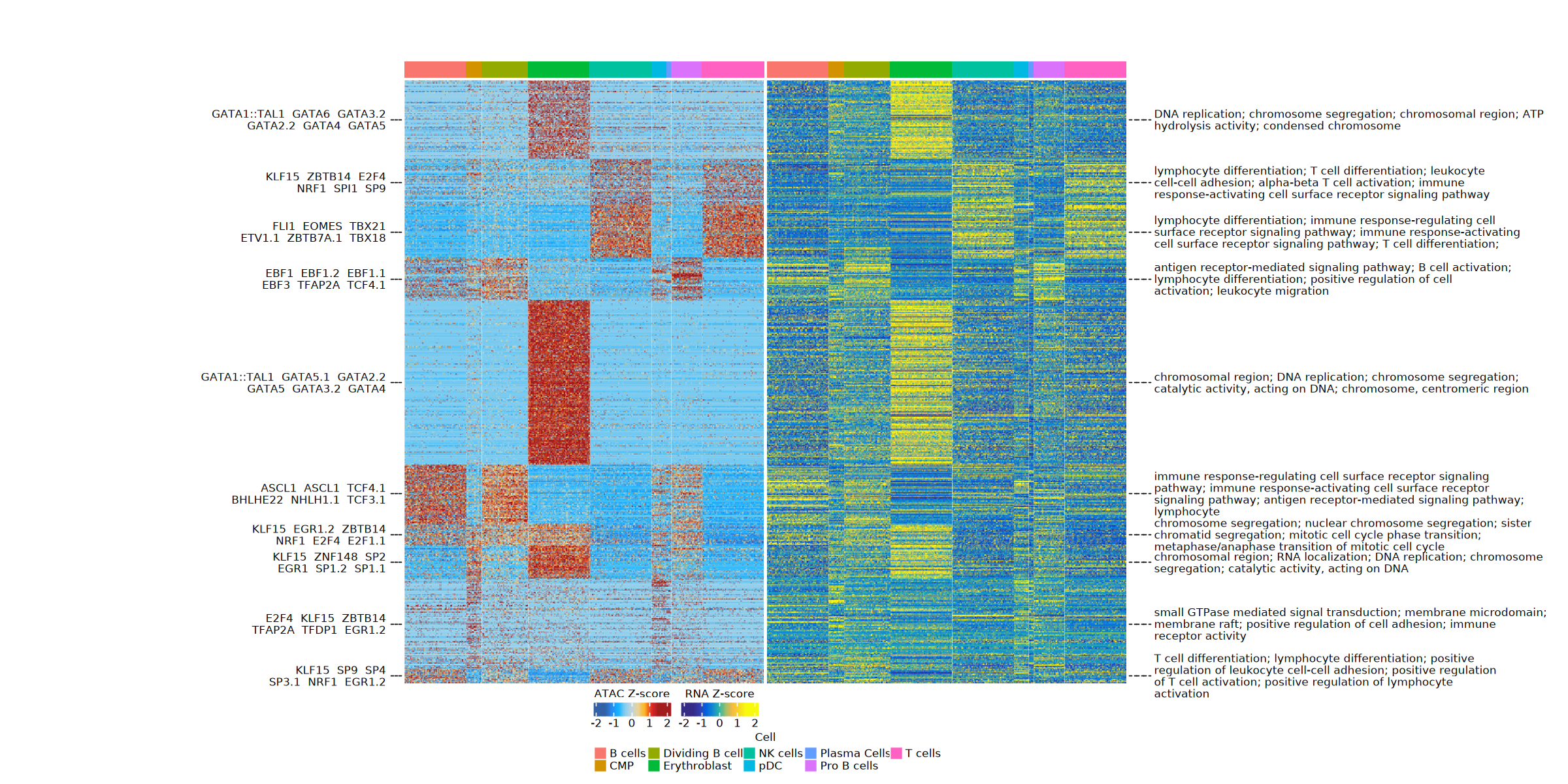

💡 Peak-to-Gene Co-Regulatory Module Joint Heatmap

This heatmap displays the correlation patterns between chromatin accessible regions and gene expression. Each row in the heatmap represents a Peak–Gene pair; each column represents a cell, and the overall row data have been partitioned by K-means clustering according to co-regulatory patterns.

• Top Color Bar: Identifies different cell types or populations, helping to intuitively compare the active patterns of Peak–Gene associations in specific cell subpopulations.
• ATAC Heatmap (Left Side of Main Plot): Shows ATAC-seq signal intensity (Z-score normalized accessibility). The bluer the color, the lower the accessibility; the redder the color, the higher the accessibility.
• RNA Heatmap (Right Side of Main Plot): Shows the expression level of the corresponding target gene (Z-score normalized expression). The bluer the color, the lower the expression; the more yellow the color, the higher the expression.
• Motif Annotation (Leftmost Text): Identifies the transcription factor binding motifs significantly enriched in each K-means cluster (Top Motifs). These TFs are often the core upstream regulators driving the gene expression of that cluster.
• GO Functional Annotation (Rightmost Text): Identifies the Gene Ontology terms significantly enriched among the target genes of each K-means cluster (Top GO Terms), intuitively revealing the core biological functions or cellular pathways engaged by that co-regulatory module.

7. Result Display and Statistics

In addition to the core clustering heatmap, you can find all enrichment result tables and link detail tables in the specified outdir directory. Furthermore, to assess the global quality of this analysis from multiple perspectives, you can invoke the following pre-defined plotting functions in the script:

• plotPeaksPerGene(links_all): Plot a histogram showing on average how many Peaks regulate each gene, evaluating the connectivity of the regulatory network.
• plotPeak2GeneVolcano(links_all): Plot a volcano plot, intuitively displaying the distributions of significance (P-value) and correlation (Correlation), highlighting core driver genes.
• plotRankCorrelation(links_all): Plot a correlation score ranking chart for all association pairs, evaluating the overall association distribution trend.

options(repr.plot.width = 10, repr.plot.height = 5)
plotPeaksPerGene(result$links)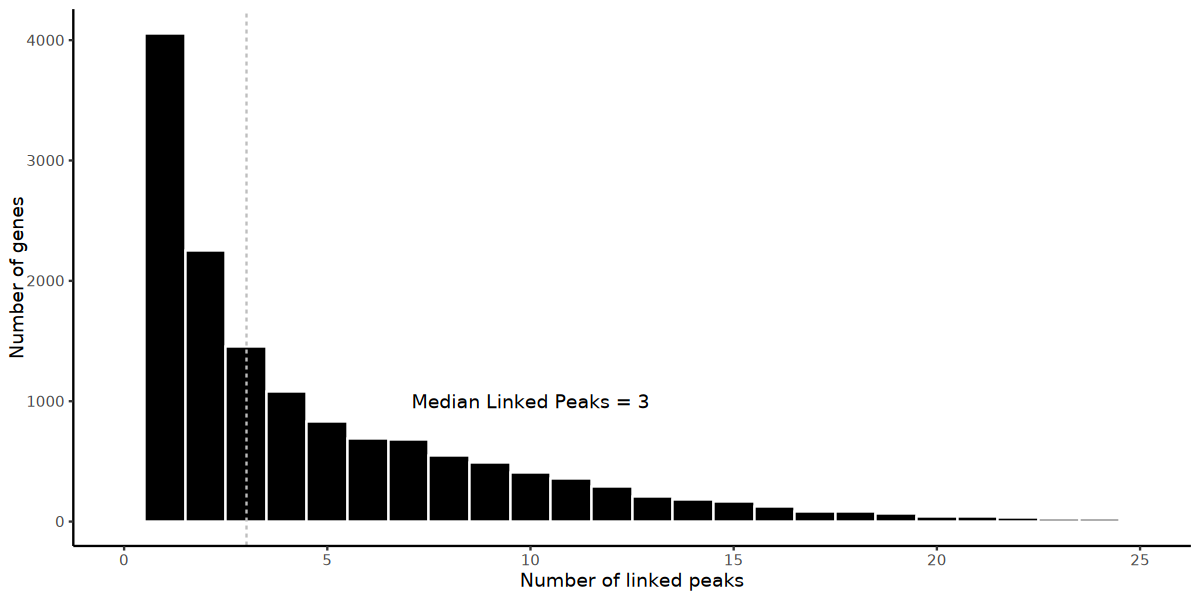

💡 Gene–Peak Association Count Distribution Histogram

This histogram primarily displays the population distribution of target genes and the number of significantly associated regulatory elements (Peaks) (by default showing the range of 1 to 25 associated Peaks).

• X-axis: Represents the number of Peaks associated with a single gene.
• Y-axis: Represents the total number of genes with the corresponding number of associated Peaks. The taller the bar, the larger the gene population with that number of regulatory elements.
• Dashed Line and Annotation: The vertical dashed line in the plot indicates the position of the median of all target genes' associated Peak counts, with the adjacent text directly labeling the specific median value. This helps quickly assess the baseline complexity of the global cis-regulatory network.

if (filter == TRUE) { 
      print(plotPeak2GeneVolcano(result$links, p = pCutOff, score = corCutOff)) 
} else { 
      print(plotPeak2GeneVolcano(result$links)) 
}

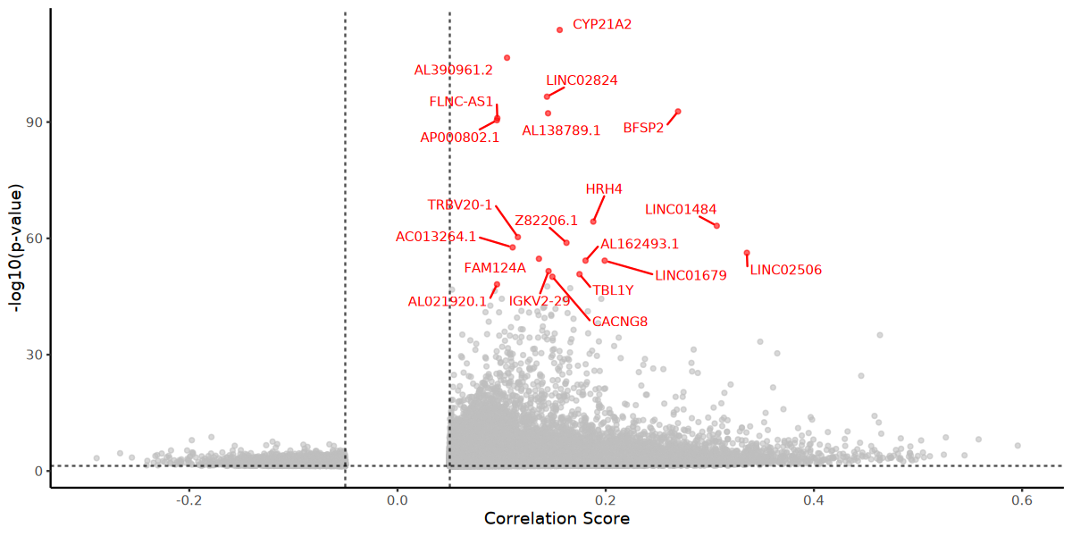
💡 Peak-to-Gene Association Volcano Plot

This volcano plot intuitively displays the correlation strength and statistical significance of all Peak–Gene association pairs, helping quickly pinpoint the most critical regulatory relationships.

• X-axis: Represents the correlation score. It indicates the degree of correlation between Peak accessibility and target gene expression; the larger the absolute value, the stronger the co-variation.
• Y-axis: Represents -log10(p-value). The higher the value, the stronger the statistical significance of that Peak–Gene association and the lower the false-positive rate.
• Text Annotation: The plot labels the gene names of the Top 10 most significant Peak–Gene associations; these genes are typically under extremely strong cis-element regulation.

print(plotRankCorrelation(result$links))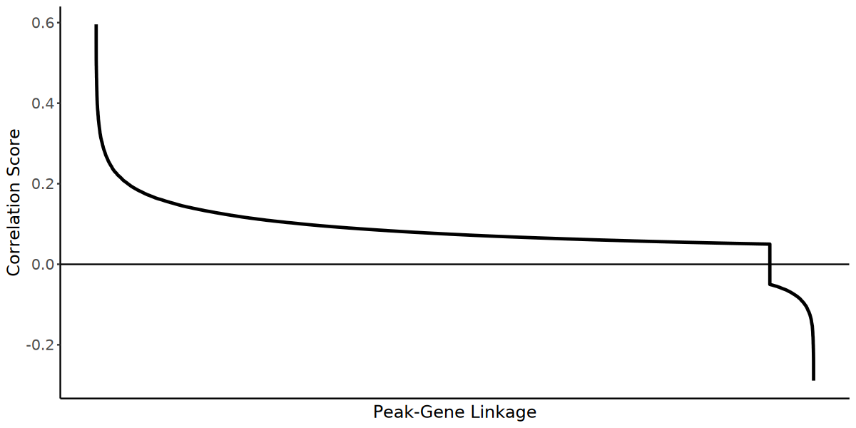

💡 Peak-to-Gene Correlation Rank Distribution Plot (Rank Correlation Plot)

This line plot provides a panoramic view of the correlation strength distribution of all detected Peak–Gene association pairs, used to intuitively assess the statistical strength and confidence threshold of the global cis-regulatory network.

• X-axis (Rank): Represents the ranking of all Peak–Gene association pairs. The system sorts all regulatory pairs in descending order of their "Correlation Score"; the higher the rank (the smaller the X-axis value), the stronger the correlation.
• Y-axis (Correlation): Represents the actual Pearson/Spearman correlation coefficient score of each Peak–Gene association pair. Positive values indicate that the opening of the Peak is accompanied by up-regulation of target gene expression (classical enhancer activation); negative values may suggest repression.
• Dashed Line and Annotation (Threshold Cutoff): The horizontal dashed line in the plot typically represents the "strong-association confidence cutoff threshold" used for subsequent downstream analysis. By observing the intersection of the curve's knee point with the dashed line, one can quickly evaluate how many high-quality regulatory pairs with strong biological significance are retained under the current filtering criteria, as well as the level of overall background noise.