
ATAC + RNA Multi-omics: SCENIC+ Multi-Omics Regulatory Network Analysis
1. Tutorial Overview
This tutorial leverages the SCENIC+ (Single-Cell Regulatory Network Inference and Clustering Plus) framework, integrating the SeekArc single-cell multi-omics dataset (RNA + ATAC), to systematically construct the complete regulatory chain of "transcription factor → cis-regulatory element → target gene."
The core advantage of SCENIC+ lies in: using chromatin accessibility information to constrain the inference of TF–target gene relationships, which significantly reduces false-positive connections compared to the traditional SCENIC method, thereby improving the interpretability of the regulatory network.
Complete Analysis Pipeline (step0 → step4):
step0: Seurat → AnnData Conversion
- Function: Extract RNA and ATAC assay counts matrices from the Seurat object, convert to AnnData (h5ad) format for downstream pycisTopic and SCENIC+ pipeline use. Also supports merging of external metadata files and optional downsampling.
- Input:
*.rds— Seurat object file (must contain both RNA and ATAC assays)meta.tsv— External metadata file (optional, TSV format, with cell-type annotation column)
- Output:
scRNA.h5ad— RNA counts matrix + cell metadata (cells × genes)scATAC.h5ad— ATAC counts matrix + cell metadata (cells × peaks, peak names standardized to chr:start-end format)
- Key Parameters:
--input_rds: Path to input Seurat RDS file--meta_path: Path to external metadata file (optional)--celltype_col: Cell-type annotation column name (defaultCellAnnotation)--output_dir: Output directory--downsample/--downsample_num: Whether to downsample and the number of cells retained per cell type
- Runtime Environment: R (Seurat + reticulate + anndata); Python environment for h5ad writing
- Script: 0_seurat_to_anndata.R
- Invocation Example:
   Rscript scripts/0_seurat_to_anndata.R \
     --input_rds /path/to/seurat_object.rds \
     --meta_path /path/to/metadata.tsv \
     --celltype_col CellAnnotation \
     --output_dir /path/to/output
step1: pycisTopic Topic Modeling
- Function: Load the ATAC counts matrix from scATAC.h5ad, build a CistopicObject, run Mallet LDA topic modeling, and output binarized topics and consensus regions BED file.
- Input:
scATAC.h5ad— ATAC AnnData output from step0*-blacklist.v2.bed— ENCODE blacklist file (selected by species)
- Output:
cistopic_obj_with_models.pkl— CistopicObject containing the LDA modelbinarized_topics.pkl— Binarized topics (DA regions for each topic)consensus_regions.bed— BED file of all regions (for step2 cisTarget use)
- Key Parameters:
--project_dir: Project root directory--species: Species name (mouse / human / fly / chicken / rat)--n_topics: Number of LDA topics (default 40)--n_iter: Number of Mallet iterations (default 500)--n_cpu: Number of parallel CPUs (default 32)
- Runtime Environment: Python (pycisTopic + Mallet)
- Script: 1_pycistopic_analysis.py
- Invocation Example:
python scripts/1_pycistopic_analysis.py \
     --project_dir /path/to/project \
     --scatac_h5ad /path/to/scATAC.h5ad \
     --blacklist /path/to/species-blacklist.v2.bed \
     --mallet_dir /path/to/mallet \
     --n_topics 40
step2: cisTarget Custom Database Construction
- Function: Based on the consensus_regions.bed output from step1, combined with reference genome FASTA and Aertslab motif collection, construct the cisTarget motif scoring database (rankings + scores) via Cluster Buster scanning, providing the required input for step3 motif enrichment analysis.
- Input:
consensus_regions.bed— Region BED file output from step1genome.fa— Reference genome FASTA (selected by species)*.chrom.sizes— Chromosome size file (selected by species)*.cb— Aertslab motif collection filecbust— Cluster Buster executable
- Output:
<species>_custom.regions_vs_motifs.rankings.feather— Motif enrichment rankings database<species>_custom.regions_vs_motifs.scores.feather— Motif enrichment scores database
- Key Parameters:
--project_dir: Project root directory--species: Species name (mouse / human / fly / chicken / rat)
- Runtime Environment: Bash + Python (cisTarget database toolchain)
- Script: 2_create_cistarget_db.sh
- Invocation Example:
bash scripts/2_create_cistarget_db.sh \
     --project_dir /path/to/project \
     --species mouse \
     --genome_fasta /path/to/genome.fa \
     --chrom_sizes /path/to/species.chrom.sizes \
     --cbust_path /path/to/cbust \
     --motif_dir /path/to/motifs/singletons \
     --script_dir /path/to/create_cisTarget_databases \
     --python_exec /path/to/python
step3: SCENIC+ Pipeline Core Inference
- Function: Integrate all outputs from steps 0–2, initialize the Snakemake pipeline, generate config.yaml, and execute regulatory network inference. Completes TF → regulatory element → target gene relationship inference, cisTarget motif enrichment, differential accessibility analysis, and AUCell activity scoring.
- Input:
scRNA.h5ad— step0 outputcistopic_obj_with_models.pkl/binarized_topics.pkl— step1 outputs<species>_custom.*.feather— step2 outputs (rankings + scores)
- Output:
scplusmdata.h5mu— Final MuData object (containing AUC matrices of direct/extended eRegulon)ctx_results.hdf5— cisTarget motif enrichment resultsdem_results.hdf5— Differential accessibility analysis resultsACC_GEX.h5mu— ATAC+GEX joint MuDatacistromes_direct.h5ad/cistromes_extended.h5ad— direct/extended cistromeAUCell_direct.h5mu/AUCell_extended.h5mu— direct/extended AUCell activity matrices- Other intermediate files: genome_annotation.tsv, search_space.tsv, eRegulons, etc.
- Key Parameters:
--project_dir: Project root directory--species: Species name (mouse / human / fly / chicken / rat)--n_cpu: Number of Snakemake parallel CPUs (default 16)--run_snakemake: Whether to automatically execute Snakemake (default only generates config)
- Runtime Environment: Python (SCENIC+ + Snakemake)
- Invocation Example (generate config only, without running Snakemake):
- Script: 3_run_scenicplus_pipeline.py
python scripts/3_run_scenicplus_pipeline.py \
     --project_dir /path/to/project \
     --scRNA_h5ad /path/to/scRNA.h5ad \
     --cistopic_obj /path/to/cistopic_obj_with_models.pkl \
     --binarized_topics /path/to/binarized_topics.pkl \
     --cistarget_dir /path/to/cisTarget \
     --motif_annotation_dir /path/to/motif_snapshots \
     --species mouse \
--n_cpu 16- Invocation Example (generate config + auto-run Snakemake):
python scripts/3_run_scenicplus_pipeline.py \
     --project_dir /path/to/project \
     --scRNA_h5ad /path/to/scRNA.h5ad \
     --cistopic_obj /path/to/cistopic_obj_with_models.pkl \
     --binarized_topics /path/to/binarized_topics.pkl \
     --cistarget_dir /path/to/cisTarget \
     --motif_annotation_dir /path/to/motif_snapshots \
     --species mouse \
     --n_cpu 16 \
     --run_snakemake
step4: SCENIC+ Data Post-Processing (Main Focus of This Tutorial)
This notebook covers the complete post-processing analysis workflow of step4, performing quality assessment, filtering, and visualization on the MuData object output from step3:
- Data Loading and Metadata Inspection: Read scplusmdata.h5mu and inspect direct/extended eRegulon metadata.
- SCENICplus Object Construction: Convert MuData to SCENIC+ internal object, integrating Cistarget and DEM results.
- eRegulon Quality Assessment and Filtering: Compute TF expression–AUC correlation, Gene/Region AUC consistency, and filter for high-quality eRegulons.
- eRegulon Similarity Analysis: Build AUC correlation heatmap and Jaccard intersection heatmap to evaluate functional redundancy.
- Regulon Specificity Score (RSS): Compute the specificity score of each eRegulon across cell types, identifying cell-type-specific regulators.
- Dimensionality Reduction and Multi-Modal Visualization: Perform UMAP/t-SNE dimensionality reduction based on eRegulon AUC matrices, mapping TF expression, Gene AUC, and Region AUC onto a common embedding.
- Joint Heatmap–Dotplot Display: Integrate RSS scores and TF expression Z-scores to construct a comprehensive regulatory feature atlas.
- Analysis Result Persistence: Serialize the complete analysis results into a pickle file for subsequent reuse.
💡 Note: The figures shown in the documentation represent only a subset of representative visualizations. For the complete analysis results across all cell types or eRegulons (including detailed data tables and all high-resolution plots), please refer to the
./result/directory.
import os
import sys
import pandas as pd
import numpy as np
import scanpy as sc
import mudata
from plotnine import *
from sklearn.preprocessing import StandardScaler
from scenicplus.RSS import regulon_specificity_scores# Parameters
#data_dir: Path to the SCENIC+ pipeline output directory, containing files such as scplusmdata.h5mu, ctx_results.hdf5, dem_results.hdf5, etc.
data_dir = '/path/to/scenicplus_pipeline'
#celltype_col: Cell-type annotation column name, used for group-based analysis and visualization coloring.
celltype_col = 'Celltype'
#R2G_positive: Whether to retain only eRegulons with R→G positive regulatory relationships (+/+ or -/+).
R2G_positive = True
#AUC_Gene_based_Region_based_cor: Minimum threshold for Gene-based and Region-based AUC correlation (default 0.5).
AUC_Gene_based_Region_based_cor = 0.5
#TF_eRegulon_cor: Absolute value threshold for TF expression–eRegulon AUC correlation (default 0.5).
TF_eRegulon_cor = 0.5
#min_target_genes: Minimum number of target genes per eRegulon, filtering out low-information regulons.
min_target_genes = 102. Data Loading and Metadata Inspection
2.1 Reading the MuData Object
Load the MuData object containing multi-omics data from the SCENIC+ pipeline output. This object integrates the RNA expression matrix, ATAC accessibility matrix, AUC matrices of direct/extended eRegulon, and rich metadata information.
import warnings
from IPython.utils.io import capture_output
from itables import init_notebook_mode
import itables.options as opt

opt.warn_on_undocumented_option = False
warnings.filterwarnings("ignore", category=SyntaxWarning, module=r"itables\.typing")

with capture_output():
init_notebook_mode(all_interactive=False)scplus_mdata = mudata.read(os.path.join(data_dir, "scplusmdata.h5mu"))from pathlib import Path
prefix = "scATAC_counts"
celltype_col_full = f"{prefix}:{celltype_col}"
outdir = Path("./result")
outdir.mkdir(parents=True, exist_ok=True)2.2 direct eRegulon Metadata Preview
Core Steps Breakdown:
- Metadata Extraction: Extract
direct_e_regulon_metadatafrom theunsattribute of MuData, containing basic information of eRegulon (TF name, number of target genes, regulatory direction, etc.). - Numerical Precision Optimization: Retain 3 significant digits for all numerical columns to improve table readability.
- Raw Data Export: Export the raw metadata as a CSV file for subsequent offline analysis or literature comparison.
💡 Note:
directeRegulon refers to the regulatory relationship in which a TF regulates target genes by directly binding to chromatin-accessible regions. This type of eRegulon has the strongest regulatory evidence and the lowest false-positive rate.
import pandas as pd
import numpy as np

df_metadata = scplus_mdata.uns["direct_e_regulon_metadata"].copy()

df_display = df_metadata.copy()

df_display.to_csv("./result/direct_e_regulon_metadata_raw.csv", index=False)

numeric_cols = df_display.select_dtypes(include=[np.number]).columns
for col in numeric_cols:
    df_display[col] = df_display[col].apply(
        lambda x: float(f"{x:.3g}") if pd.notnull(x) else x
    )

print("DataFrame shape:", df_display.shape)

print(df_display.head())--- 前 5 行 ---
Region Gene importance_R2G rho_R2G importance_x_rho \\
0 chr5:180815523-180816104 MGAT1 0.1440 0.2190 0.0316
1 chr7:73594104-73594910 TBL2 0.0310 0.0969 0.0030
2 chr6:158995255-158995808 TAGAP 0.0518 0.0907 0.0047
3 chr11:47390837-47391602 SPI1 0.0879 0.6070 0.0533
4 chr2:144412741-144415133 ZEB2 0.0593 0.2640 0.0157
importance_x_abs_rho TF is_extended eRegulon_name \\
0 0.0316 BACH1 False BACH1_direct_+/+
1 0.0030 BACH1 False BACH1_direct_+/+
2 0.0047 BACH1 False BACH1_direct_+/+
3 0.0533 BACH1 False BACH1_direct_+/+
4 0.0157 BACH1 False BACH1_direct_+/+
Gene_signature_name Region_signature_name importance_TF2G \\
0 BACH1_direct_+/+_(813g) BACH1_direct_+/+_(1732r) 3.230
1 BACH1_direct_+/+_(813g) BACH1_direct_+/+_(1732r) 0.915
2 BACH1_direct_+/+_(813g) BACH1_direct_+/+_(1732r) 1.250
3 BACH1_direct_+/+_(813g) BACH1_direct_+/+_(1732r) 1.260
4 BACH1_direct_+/+_(813g) BACH1_direct_+/+_(1732r) 2.480
regulation rho_TF2G triplet_rank
0 1.0 0.388 7740.0
1 1.0 0.181 57800.0
2 1.0 0.205 36000.0
3 1.0 0.524 24300.0
4 1.0 0.553 48800.0
2.3 extended eRegulon Metadata Preview
Similar to direct eRegulon, extended eRegulon infers TF–target gene relationships through indirect information such as gene distance or chromatin interactions. This type of eRegulon covers a broader range, but its evidence strength is slightly lower than that of the direct type. Comparative analysis of the two helps distinguish direct from indirect regulatory signals.
df_metadata_ext = scplus_mdata.uns["extended_e_regulon_metadata"].copy()

df_display_ext = df_metadata_ext.copy()
df_display_ext.to_csv("./result/extended_e_regulon_metadata_raw.csv", index=False)

numeric_cols_ext = df_display_ext.select_dtypes(include=[np.number]).columns
for col in numeric_cols_ext:
    df_display_ext[col] = df_display_ext[col].apply(
        lambda x: float(f'{x:.3g}') if pd.notnull(x) else x
    )

print("Extended DataFrame shape:", df_display_ext.shape)
print(df_display_ext.head())--- 前 5 行 ---
Region Gene importance_R2G rho_R2G \\
0 chr4:138241948-138242957 SLC7A11 0.0890 0.106
1 chr14:75301587-75302301 FOS 0.0414 0.429
2 chr2:27010539-27011332 TMEM214 0.0735 0.115
3 chr7:112509759-112511021 IFRD1 0.0585 0.152
4 chr14:68732843-68733669 ACTN1 0.0572 0.510
importance_x_rho importance_x_abs_rho TF is_extended \\
0 0.00942 0.00942 ATF4 True
1 0.01780 0.01780 ATF4 True
2 0.00849 0.00849 ATF4 True
3 0.00890 0.00890 ATF4 True
4 0.02920 0.02920 ATF4 True
eRegulon_name Gene_signature_name Region_signature_name \\
0 ATF4_extended_+/+ ATF4_extended_+/+_(21g) ATF4_extended_+/+_(22r)
1 ATF4_extended_+/+ ATF4_extended_+/+_(21g) ATF4_extended_+/+_(22r)
2 ATF4_extended_+/+ ATF4_extended_+/+_(21g) ATF4_extended_+/+_(22r)
3 ATF4_extended_+/+ ATF4_extended_+/+_(21g) ATF4_extended_+/+_(22r)
4 ATF4_extended_+/+ ATF4_extended_+/+_(21g) ATF4_extended_+/+_(22r)
importance_TF2G regulation rho_TF2G triplet_rank
0 1.430 1.0 0.129 4600.0
1 0.746 1.0 0.449 33600.0
2 0.823 1.0 0.156 22000.0
3 0.907 1.0 0.271 24500.0
4 0.891 1.0 0.232 23800.0
3. SCENICplus Object Construction
3.1 MuData to SCENICplus Object Conversion
Core Steps Breakdown:
- Cistarget Result Integration: Load the CuB (Cis-regulatory element target binding) database motif enrichment results, linking TF motifs to chromatin-accessible regions.
- DEM Result Integration: Load the Differential Enrichment Matrix analysis results to identify cell-type-specific regulatory elements.
- Object Conversion: Convert the multi-omics data in MuData format to the SCENIC+ internal object structure, preparing for downstream eRegulon quality control and filtering.
⚠️ Note: The
mudata_to_scenicplusfunction requires the input MuData object to contain the complete SCENIC+ pipeline output modalities (scRNA_counts, scATAC_counts, various AUC matrices, etc.). If the MuData structure is incomplete, the conversion will raise a KeyError.
from scenicplus.scenicplus_class import mudata_to_scenicplusscplus_obj = mudata_to_scenicplus(
mdata = scplus_mdata,
path_to_cistarget_h5 = os.path.join(data_dir, "ctx_results.hdf5"),
path_to_dem_h5 = os.path.join(data_dir, "dem_results.hdf5")
)import numpy as np
import pandas as pd
from scenicplus.regulon_qc.quality_metrics import calculate_correlation
import pandas as pd
import re
import numpy as np
import matplotlib.pyplot as plt
import seaborn as sns
def generate_pseudobulks_fixed(
scplus_mudata,
variable,
modality,
nr_cells_to_sample=10,
nr_pseudobulks_to_generate=100,
seed=555,
normalize_data=False
):
if variable not in scplus_mudata.obs.columns:
raise ValueError(f"{variable} not in scplus_mudata.obs.columns")
if modality not in scplus_mudata.mod.keys():
raise ValueError(f"{modality} not in scplus_mudata.mod.keys()")
np.random.seed(seed)
data_matrix = scplus_mudata[modality].to_df()
if normalize_data:
libsize = data_matrix.sum(axis=1).replace(0, np.nan)
data_matrix = np.log1p(data_matrix.div(libsize, axis=0) * 1e6).fillna(0)
variable_to_cells = (
scplus_mudata.obs.groupby(variable).apply(lambda x: list(x.index)).to_dict()
)
variable_to_mean_data = {}
for group, cells in variable_to_cells.items():
num_to_sample = min(nr_cells_to_sample, len(cells))
if len(cells) == 0:
continue
for i in range(nr_pseudobulks_to_generate):
sampled_cells = np.random.choice(cells, size=num_to_sample, replace=False)
variable_to_mean_data[f"{group}_{i}"] = data_matrix.loc[sampled_cells].mean(axis=0)
return pd.DataFrame(variable_to_mean_data).T(1) Target Gene Number Extraction Function Extract the number of target genes from the eRegulon name (e.g., "TF_+/+(150g)" → 150), for use as the y-axis in subsequent quality scatter plots.
def extract_n_targets(reg_name):
    m = re.search(r"\((\d+)[gr]\)$", str(reg_name))
    return int(m.group(1)) if m else np.nan
(2) TF Expression Pseudo-Bulk Construction Generate pseudo-bulk samples by grouping the TF expression matrix by cell type, and apply log1p(CPM) normalization to eliminate sequencing depth differences.
expr_pb = generate_pseudobulks_fixed(
    scplus_mudata=scplus_mdata,
    variable=celltype_col_full,
    modality='scRNA_counts',
    nr_cells_to_sample=10,
    nr_pseudobulks_to_generate=100,
    seed=555,
    normalize_data=True
)

df_direct = None
df_extended = None
modalities = ['direct_gene_based_AUC', 'extended_gene_based_AUC']

for modality in modalities:
    auc_pb = generate_pseudobulks_fixed(
        scplus_mudata=scplus_mdata,
        variable=celltype_col_full,
        modality=modality,
        nr_cells_to_sample=10,
        nr_pseudobulks_to_generate=100,
        seed=555,
        normalize_data=False
    )

    common_idx = expr_pb.index.intersection(auc_pb.index)
    expr_sub = expr_pb.loc[common_idx]
    auc_sub = auc_pb.loc[common_idx]

    reg_to_tf = {reg: reg.split('_(')[0].split('_')[0] for reg in auc_sub.columns}
    valid_regs = [reg for reg, tf in reg_to_tf.items() if tf in expr_sub.columns]

    A = pd.DataFrame({reg: expr_sub[reg_to_tf[reg]] for reg in valid_regs}, index=expr_sub.index)
    B = auc_sub[valid_regs]
    mapping = {reg: reg for reg in valid_regs}

    df_corr = calculate_correlation(A=A, B=B, mapping_A_to_B=mapping)
    df_corr['n_targets'] = df_corr['B'].map(extract_n_targets)

    if modality == 'direct_gene_based_AUC':
        df_direct = df_corr
    else:
        df_extended = df_corr
3.2 TF Expression–AUC Correlation Visualization
Place the quality assessment results of both direct and extended eRegulons on the same page for comparison.
Core Steps Breakdown:
- Unified Threshold: Use
TF_eRegulon_coras the correlation threshold, marking the boundary of high-quality eRegulon in the plot. - Significance Encoding: Use
-log10(adjusted p-value)as the scatter point color, simultaneously displaying both correlation and statistical significance. - Dual-Panel Comparison: Left panel shows direct eRegulon; right panel shows extended eRegulon — providing an intuitive evaluation of the quality distribution differences between the two regulatory evidence types.
fig, axes = plt.subplots(1, 2, figsize=(11, 5))
datasets = [
    (df_direct, 'Direct eRegulons'),
    (df_extended, 'Extended eRegulons')
]

rho_thresh = TF_eRegulon_cor
thresholds = {"rho": [-rho_thresh, rho_thresh]}

for i, (df, title) in enumerate(datasets):
    ax = axes[i]
    if df is None or df.empty:
        ax.text(0.5, 0.5, f"No data for {title}", transform=ax.transAxes, ha='center')
        continue

    df_clean = df.dropna(subset=['rho', 'n_targets']).copy()
    df_clean['adj_pval'] = df_clean['pval_adj'].clip(lower=1e-300)

    sc = ax.scatter(
        df_clean['rho'],
        df_clean['n_targets'],
        c=-np.log10(df_clean['adj_pval']),
        s=8
    )

    ax.set_xlabel("Correlation coefficient")
    ax.set_ylabel("nr. targets")
    ax.set_title(title, fontweight='bold')

    ax.vlines(
        x=thresholds["rho"],
        ymin=0,
        ymax=df_clean['n_targets'].max(),
        colors='black',
        linestyles='dashed',
        linewidths=1
    )
    for thresh in thresholds["rho"]:
        ax.text(thresh, df_clean['n_targets'].max(), str(thresh), va='bottom', ha='center', fontsize=9)

    sns.despine(ax=ax)

#cbar = fig.colorbar(sc, ax=axes, shrink=0.95, pad=0.2)
cax = fig.add_axes([1, 0.15, 0.02, 0.7])
cbar = fig.colorbar(sc, cax=cax)
#cbar = fig.colorbar(sc, ax=axes, location='right', shrink=0.9, pad=0.02)
cbar.set_label('-log10(adjusted p-value)', rotation=270, labelpad=20)

plt.tight_layout()
save_path = "./result/TF_eRegulon_cor_Direct_vs_Extended.pdf"
plt.savefig(save_path, bbox_inches='tight')

plt.show()
plt.close(fig)/tmp/ipykernel_1828/996563594.py:55: UserWarning: This figure includes Axes that are not compatible with tight_layout, so results might be incorrect.
/tmp/ipykernel_1828/996563594.py:55: UserWarning: This figure includes Axes that are not compatible with tight_layout, so results might be incorrect.
/PROJ2/FLOAT/shumeng/apps/miniconda3/envs/scenicplus/lib/python3.11/site-packages/IPython/core/pylabtools.py:170: UserWarning: This figure includes Axes that are not compatible with tight_layout, so results might be incorrect.
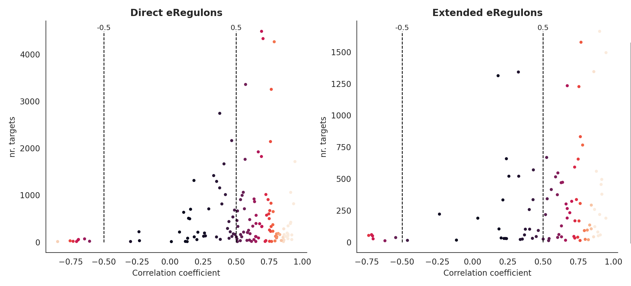
💡 Interpretation Guide
Global Description: The scatter plot displays the TF expression–AUC correlation (x-axis) and number of target genes (y-axis) for all eRegulons, with color indicating statistical significance.
- X-axis (Correlation coefficient): Pearson correlation coefficient between TF expression and eRegulon AUC value. The higher the positive value, the more the increase in TF expression is accompanied by an increase in target gene regulatory activity, making the regulatory relationship more credible.
- Y-axis (nr. targets): Number of target genes contained in the eRegulon.
- Dashed threshold: Boundary lines of
±TF_eRegulon_cor. eRegulons falling outside the dashed lines are high-quality regulatory relationships and will be retained for downstream analysis.- Color gradient: The brighter the color, the larger the
-log10(p-value), i.e., the higher the statistical significance.
4. eRegulon Consistency Filtering
4.1 Gene-based and Region-based AUC Consistency Filtering
To obtain highly reliable eRegulons, the program performs a consistency assessment on the two AUC computation modes — Gene-based and Region-based — and applies strict filtering based on multiple criteria including R2G regulatory direction and number of target genes.
Core Steps Breakdown:
- Base Name Normalization: Simplify the eRegulon name to the base TF name (e.g.,
STAT1_+_direct_(150g)→STAT1) for alignment between Gene- and Region-based computation modes. - Consistency Filtering: Compute the Pearson correlation between Gene-based and Region-based AUC for each eRegulon, retaining only those with
|correlation| > AUC_Gene_based_Region_based_cor. This ensures that two independent AUC computation methods yield consistent results. - R2G Direction Filtering: When
R2G_positive = True, retain only positive regulatory relationships (+/+ or -/+), excluding reverse regulatory ones (+/− or −/−), which may represent indirect or repressive regulation. - Direct vs Extended De-Redundancy: If both direct and extended versions of the same TF exist simultaneously, retain only the direct version to avoid duplication.
- Target Gene Count Filtering: Retain only eRegulons with more than
min_target_genestarget genes, filtering out low-information regulatory relationships. - Signature Extraction: Based on the filtered eRegulons, generate Gene-based and Region-based target gene signatures for downstream enrichment analysis.
💡 Note:
- Gene-based AUC: AUC computed based on the target gene expression matrix, reflecting the regulatory activity of the eRegulon at the gene expression level.
- Region-based AUC: AUC computed based on chromatin-accessible regions, reflecting the regulatory activity of the eRegulon at the chromatin level.
- The higher the consistency between the two, the stronger the reliability — indicating that the eRegulon's regulatory signal can be independently validated across multiple omics layers.
(1) eRegulon Base Name Extraction Simplify the full eRegulon name to the base TF name, for alignment between the Gene-based and Region-based AUC matrices.
def _eregulon_base_name(x):
    return str(x).split("_(")[0]
(2) Target Gene Count Extraction (Gene-based) Extract the number of target genes from the Gene-based eRegulon column names, used for filtering out low-information regulatory relationships.
def _gene_targets_from_eregulon_col(x):
    m = re.search(r"\((\d+)g\)$", str(x))
return int(m.group(1)) if m else Noneauc_container = scplus_obj.uns.get("eRegulon_AUC")
if auc_container is None:
raise KeyError("scplus_obj.uns does not contain 'eRegulon_AUC'")
if "Gene_based" not in auc_container or "Region_based" not in auc_container:
raise KeyError("scplus_obj.uns['eRegulon_AUC'] must contain 'Gene_based' and 'Region_based'")
df1 = auc_container["Gene_based"].copy()
df2 = auc_container["Region_based"].copy()
df1_base = df1.copy()
df2_base = df2.copy()
df1_base.columns = [_eregulon_base_name(c) for c in df1_base.columns]
df2_base.columns = [_eregulon_base_name(c) for c in df2_base.columns]
df1_base = df1_base.groupby(level=0, axis=1).mean()
df2_base = df2_base.groupby(level=0, axis=1).mean()
common = sorted(set(df1_base.columns).intersection(df2_base.columns))
if len(common) == 0:
raise ValueError("No overlapping eRegulon base names between Gene_based and Region_based AUC matrices")
correlations = df1_base[common].corrwith(df2_base[common], axis=0)
correlations = correlations[abs(correlations) > AUC_Gene_based_Region_based_cor]
if R2G_positive:
keep_base = [x for x in correlations.index if ("+/+" in x) or ("-/+" in x)]
print(f"[Debug] Remaining after R2G_positive filtering (+/+ or -/+): {len(keep_base)}")
else:
keep_base = list(correlations.index)
extended = [x for x in keep_base if "extended" in str(x)]
direct = [x for x in keep_base if "extended" not in str(x)]
keep_extended = [x for x in extended if x.replace("_extended", "_direct") not in direct]
keep_base = direct + keep_extended
keep_gene = [
x for x in auc_container["Gene_based"].columns
if _eregulon_base_name(x) in keep_base
]
keep_gene = [
x for x in keep_gene
if (_gene_targets_from_eregulon_col(x) is not None) and (_gene_targets_from_eregulon_col(x) > min_target_genes)
]
keep_region = [
x for x in auc_container["Region_based"].columns
if _eregulon_base_name(x) in keep_base
]
keep_gene_base = {_eregulon_base_name(x) for x in keep_gene}
keep_region = [x for x in keep_region if _eregulon_base_name(x) in keep_gene_base]
scplus_obj.uns["selected_eRegulons"] = {"Gene_based": keep_gene, "Region_based": keep_region}4.2 eRegulon Extraction
Convert the filtered eRegulons into a list of target gene signatures for subsequent similarity analysis (Jaccard intersection). Each eRegulon corresponds to a target gene set; signatures can undergo intersection/union operations to evaluate functional redundancy.
from scenicplus.eregulon_enrichment import get_eRegulons_as_signatures

scplus_obj.uns["eRegulon_signatures"] = get_eRegulons_as_signatures(
    eRegulons=scplus_obj.uns["eRegulon_metadata"]
)
gene_sig_pool = scplus_obj.uns["eRegulon_signatures"]["Gene_based"]
region_sig_pool = scplus_obj.uns["eRegulon_signatures"]["Region_based"]

selected_base = set(
    [_eregulon_base_name(x) for x in scplus_obj.uns["selected_eRegulons"]["Gene_based"]]
    + [_eregulon_base_name(x) for x in scplus_obj.uns["selected_eRegulons"]["Region_based"]]
)
final_gene_sig = [k for k in gene_sig_pool.keys() if _eregulon_base_name(k) in selected_base]
final_region_sig = [k for k in region_sig_pool.keys() if _eregulon_base_name(k) in selected_base]

scplus_obj.uns["selected_eRegulon"] = {"Gene_based": final_gene_sig, "Region_based": final_region_sig}
5. eRegulon Similarity Analysis
5.1 AUC Correlation Heatmap Construction
After eRegulon filtering, to further evaluate the functional redundancy among eRegulons, the program computes the Pearson correlation based on the AUC matrix and generates a heatmap combined with hierarchical clustering.
Core Steps Breakdown:
- Matrix Concatenation and Normalization: Concatenate AUC matrices of the specified signature_keys (e.g., Gene-based) column-wise. When
scale=True, apply Z-score normalization to the data to eliminate dimensional differences. - All-Zero Column Filtering: Remove eRegulons with AUC sum equal to 0 (inactive in the target cell types) to avoid interfering with clustering.
- Distance Matrix and Hierarchical Clustering: Use
1 - correlationas the distance metric and apply hierarchical clustering withaveragelinkage. Cut the dendrogram at the specified threshold viafcluster, grouping similar eRegulons into the same cluster. - Cluster-Rearranged Heatmap: Sort eRegulons by cluster labels so that functionally similar eRegulons appear adjacent in the heatmap, facilitating the identification of regulatory modules.
5.2 Jaccard Intersection Heatmap Construction
In addition to AUC-value-based correlation, the program also evaluates eRegulon similarity at the target gene set level. The Jaccard coefficient measures the ratio of the intersection to the union of two eRegulons' target gene sets, directly reflecting the overlap in regulatory targets.
Core Steps Breakdown:
- Jaccard Coefficient Calculation: For each pair of eRegulons, compute their target gene set Jaccard index = |A∩B| / |A∪B|. The value range is [0, 1]; the higher the value, the more similar the target genes of the two eRegulons.
- Intersection Normalization (Optional): When
method='intersect', use the first eRegulon's target gene set as denominator to compute the intersection proportion, generating an asymmetric matrix. - Symmetrization: Apply
(M + M^T) / 2symmetrization to theintersectmethod to ensure reasonable clustering results. - Hierarchical Clustering and Heatmap: The same clustering workflow as the correlation heatmap, but with distance metric based on
1 - Jaccard.
from itertools import combinations
import numpy as np
import pandas as pd
import matplotlib.pyplot as plt
import seaborn as sns
import sklearn

from scipy.cluster.hierarchy import linkage, fcluster
from scipy.spatial.distance import squareform


def custom_correlation_heatmap(
    scplus_obj,
    auc_key='eRegulon_AUC',
    signature_keys=['Gene_based'],
    scale=False,
    linkage_method='average',
    fcluster_threshold=0.1,
    selected_regulons=None,
    cmap='viridis',
    fontsize=10,
    ax=None
):
    if scale:
        data_mat = pd.concat([
            pd.DataFrame(
                sklearn.preprocessing.StandardScaler().fit_transform(
                    scplus_obj.uns[auc_key][x].T
                ),
                index=scplus_obj.uns[auc_key][x].T.index.to_list(),
                columns=scplus_obj.uns[auc_key][x].T.columns
            )
            for x in signature_keys
        ]).T
    else:
        data_mat = pd.concat(
            [scplus_obj.uns[auc_key][x] for x in signature_keys],
            axis=1
        )

    if selected_regulons is not None:
        subset = [x for x in selected_regulons if x in data_mat.columns]
        data_mat = data_mat[subset]

    all_zero_eregs = data_mat.columns[np.where(data_mat.sum(axis=0) == 0)]
    if len(all_zero_eregs) > 0:
        data_mat = data_mat.drop(columns=all_zero_eregs)

    correlations = data_mat.corr()
    similarity = 1 - correlations

    similarity = (similarity + similarity.T) / 2
    np.fill_diagonal(similarity.values, 0)

    Z = linkage(
        np.clip(squareform(similarity), 0, similarity.to_numpy().max()),
        method=linkage_method
    )
    labels = fcluster(Z, fcluster_threshold, criterion='distance')
    labels_order = np.argsort(labels)

    clustered = data_mat.iloc[:, labels_order]
    correlations = clustered.corr()

    if ax is None:
        fig, ax = plt.subplots(figsize=(10, 10))

    sns.heatmap(
        data=correlations,
        cmap=cmap,
        square=True,
        ax=ax,
        robust=True,
        cbar=True,
        cbar_kws={"shrink": 0.75, "label": "Correlation"},
        xticklabels=True,
        yticklabels=True
    )

    ax.tick_params(axis='x', labelsize=fontsize, rotation=90)
    ax.tick_params(axis='y', labelsize=fontsize, rotation=0)
    ax.set_title("Correlation heatmap", fontsize=fontsize + 2, fontweight='bold')

    return ax


def _jaccard(signature1, signature2):
    s_signature1 = set(signature1)
    s_signature2 = set(signature2)
    intersect = len(s_signature1 & s_signature2)
    union = len(s_signature1) + len(s_signature2) - intersect
    return intersect / union if union != 0 else 0


def _intersect_norm_by_one(signature1, signature2):
    s_signature1 = set(signature1)
    s_signature2 = set(signature2)
    intersect = len(s_signature1 & s_signature2)
    return intersect / len(s_signature1) if len(s_signature1) != 0 else 0


def custom_jaccard_heatmap(
    scplus_obj,
    method='jaccard',
    gene_or_region_based='Gene_based',
    signature_key='eRegulon_signatures',
    selected_regulons=None,
    linkage_method='average',
    fcluster_threshold=0.1,
    cmap='viridis',
    fontsize=10,
    vmin=None,
    vmax=None,
    ax=None
):
    signatures = scplus_obj.uns[signature_key][gene_or_region_based]

    if selected_regulons is not None:
        signatures = {k: signatures[k] for k in signatures.keys() if k in selected_regulons}

    signatures_names = list(signatures.keys())
    n_signatures = len(signatures_names)

    jaccards = np.zeros((n_signatures, n_signatures), dtype=float)

    for i, signature_1 in enumerate(signatures_names):
        for j, signature_2 in enumerate(signatures_names):
            if i == j:
                jaccards[i, j] = 1.0
            else:
                if method == 'jaccard':
                    jaccards[i, j] = _jaccard(signatures[signature_1], signatures[signature_2])
                elif method == 'intersect':
                    jaccards[i, j] = _intersect_norm_by_one(
                        signatures[signature_1], signatures[signature_2]
                    )
                else:
                    raise ValueError("method must be 'jaccard' or 'intersect'")

    if method == 'intersect':
        cluster_mat = (jaccards + jaccards.T) / 2
    else:
        cluster_mat = jaccards.copy()

    similarity = 1 - cluster_mat
    similarity = (similarity + similarity.T) / 2
    np.fill_diagonal(similarity, 0)

    Z = linkage(squareform(similarity), method=linkage_method)
    labels = fcluster(Z, fcluster_threshold, criterion='distance')
    labels_order = np.argsort(labels)

    clustered_df = pd.DataFrame(
        jaccards,
        index=signatures_names,
        columns=signatures_names
    ).iloc[labels_order, labels_order]

    if ax is None:
        fig, ax = plt.subplots(figsize=(10, 10))

    sns.heatmap(
        data=clustered_df,
        cmap=cmap,
        square=True,
        ax=ax,
        robust=True,
        cbar=True,
        cbar_kws={
            "shrink": 0.75,
            "label": "Jaccard" if method == 'jaccard' else 'Intersection'
        },
        xticklabels=True,
        yticklabels=True,
        vmin=vmin,
        vmax=vmax
    )

    ax.tick_params(axis='x', labelsize=fontsize, rotation=90)
    ax.tick_params(axis='y', labelsize=fontsize, rotation=0)
    ax.set_title(
        "Jaccard heatmap" if method == 'jaccard' else "Intersection heatmap",
        fontsize=fontsize + 2,
        fontweight='bold'
    )

    return ax
5.3 Dual-Panel Heatmap Output
Place the AUC correlation heatmap and the Jaccard intersection heatmap side by side, comprehensively evaluating eRegulon similarity from both continuous-value and set perspectives.
sns.set_style("white")

fig, axes = plt.subplots(
    1, 2,
    figsize=(26, 13)
    #constrained_layout=True
)

selected_regs = scplus_obj.uns['selected_eRegulons']['Gene_based']

custom_correlation_heatmap(
    scplus_obj,
    auc_key='eRegulon_AUC',
    signature_keys=['Gene_based'],
    scale=False,
    selected_regulons=selected_regs,
    linkage_method='average',
    fcluster_threshold=0.1,
    cmap='viridis',
    fontsize=10,
    ax=axes[0]
)

custom_jaccard_heatmap(
    scplus_obj,
    method='intersect',
    gene_or_region_based='Gene_based',
    signature_key='eRegulon_signatures',
    selected_regulons=selected_regs,
    linkage_method='average',
    fcluster_threshold=0.1,
    cmap='viridis',
    fontsize=10,
    vmin=None,
    vmax=None,
    ax=axes[1]
)

save_path = "./result/correlation_and_intersection_heatmaps.pdf"
plt.savefig(save_path, format="pdf", bbox_inches="tight")

plt.show()
plt.close(fig)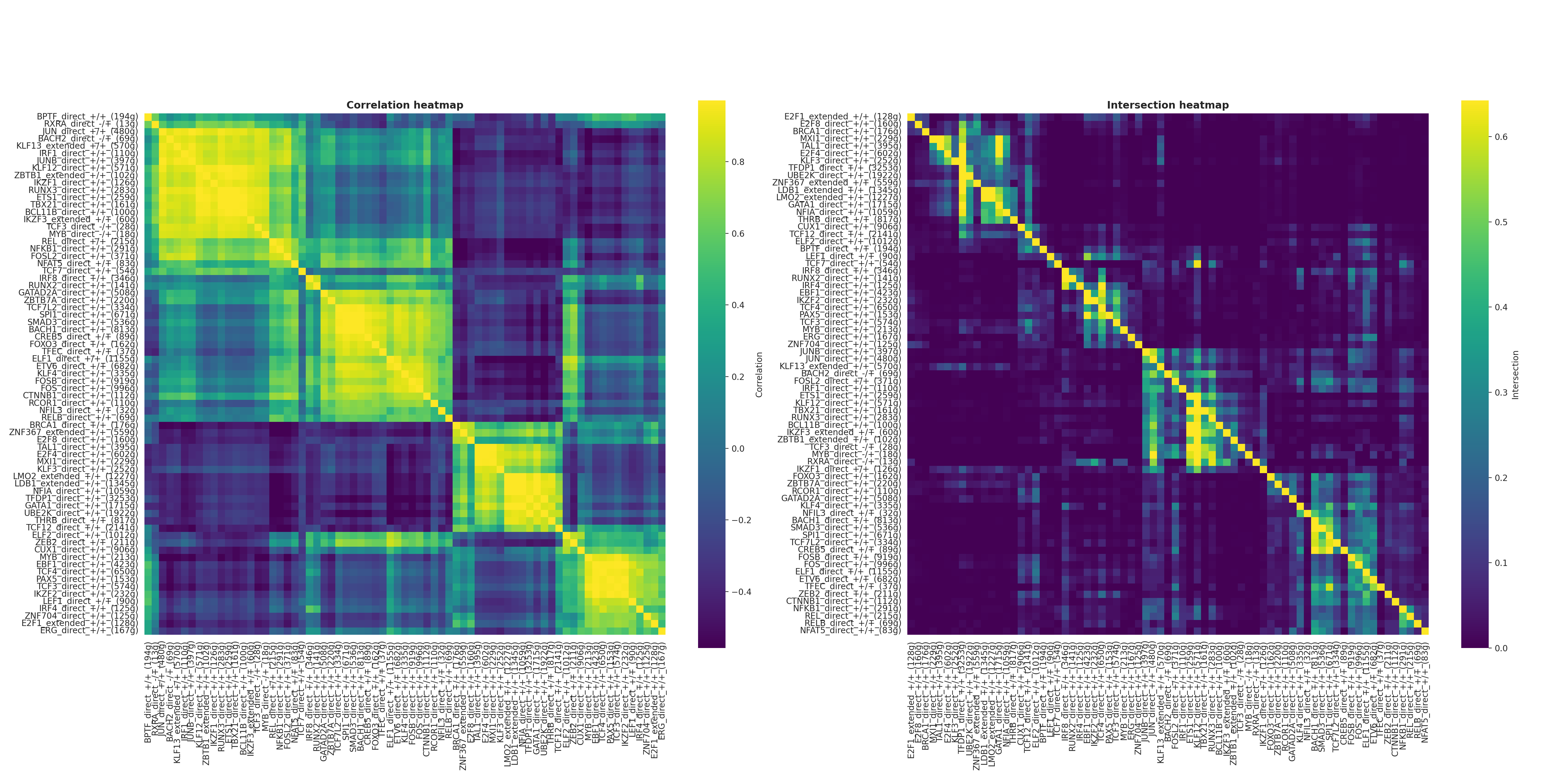
💡 Interpretation Guide
Global Description: Left is the AUC correlation heatmap; right is the intersection proportion heatmap. Both heatmaps share the same eRegulon ordering (hierarchical clustering result).
- AUC Correlation Heatmap: Reflects whether eRegulons have similar activity patterns across cells. Highly correlated eRegulons may regulate the same pathway or reside at the same regulatory level.
- Intersection Heatmap (Intersect): Reflects the degree of target gene overlap among eRegulons. eRegulons with high intersection may have functional redundancy or serve as backups for each other.
- Joint Interpretation: If two eRegulons are highly similar in both heatmaps, they likely represent different aspects of the same regulatory axis; if they are similar only in the AUC heatmap but have non-overlapping target genes, this may suggest an indirect regulatory relationship.
6. Regulon Specificity Score (RSS)
6.1 MuData Filtering and Consistency Alignment
Before computing the Regulon Specificity Score, the eRegulon filtering results from previous steps must be propagated back into the MuData object to ensure RSS computation is based only on high-quality eRegulons.
Core Steps Breakdown:
- Consistency Intersection: Take the intersection of base names of eRegulons retained on both Gene-based and Region-based sides as a unified filtering criterion.
- Four-Modality Filtering: Perform variable filtering separately on the four AUC modalities (direct/extended × gene/region) to ensure consistency in downstream analyses.
- AUC Matrix Concatenation: Concatenate the direct and extended Gene-based/Region-based AUC matrices respectively into unified AnnData objects, preparing for downstream dimensionality reduction visualization.
from scenicplus.RSS import (regulon_specificity_scores, plot_rss)
import anndata

selected_gene_regulons = scplus_obj.uns['selected_eRegulons']['Gene_based']
selected_region_regulons = scplus_obj.uns['selected_eRegulons']['Region_based']

selected_gene_base = {_eregulon_base_name(x) for x in selected_gene_regulons}
selected_region_base = {_eregulon_base_name(x) for x in selected_region_regulons}
selected_base_consensus = selected_gene_base.intersection(selected_region_base)

keep_gene_vars_direct = [v for v in scplus_mdata["direct_gene_based_AUC"].var_names
                         if _eregulon_base_name(v) in selected_base_consensus]
keep_gene_vars_extended = [v for v in scplus_mdata["extended_gene_based_AUC"].var_names
                           if _eregulon_base_name(v) in selected_base_consensus]
keep_region_vars_direct = [v for v in scplus_mdata["direct_region_based_AUC"].var_names
                           if _eregulon_base_name(v) in selected_base_consensus]
keep_region_vars_extended = [v for v in scplus_mdata["extended_region_based_AUC"].var_names
                             if _eregulon_base_name(v) in selected_base_consensus]

scplus_mdata_filt = scplus_mdata.copy()
scplus_mdata_filt.mod["direct_gene_based_AUC"] = scplus_mdata_filt.mod["direct_gene_based_AUC"][:, keep_gene_vars_direct]
scplus_mdata_filt.mod["extended_gene_based_AUC"] = scplus_mdata_filt.mod["extended_gene_based_AUC"][:, keep_gene_vars_extended]
scplus_mdata_filt.mod["direct_region_based_AUC"] = scplus_mdata_filt.mod["direct_region_based_AUC"][:, keep_region_vars_direct]
scplus_mdata_filt.mod["extended_region_based_AUC"] = scplus_mdata_filt.mod["extended_region_based_AUC"][:, keep_region_vars_extended]
scplus_mdata_filt.update()

eRegulon_gene_AUC = anndata.concat(
    [scplus_mdata_filt["direct_gene_based_AUC"], scplus_mdata_filt["extended_gene_based_AUC"]],
    axis=1,
)
eRegulon_gene_AUC.obs = scplus_mdata_filt.obs.loc[eRegulon_gene_AUC.obs_names].copy()

eRegulon_region_AUC = anndata.concat(
    [scplus_mdata_filt["direct_region_based_AUC"], scplus_mdata_filt["extended_region_based_AUC"]],
    axis=1,
)
eRegulon_region_AUC.obs = scplus_mdata_filt.obs.loc[eRegulon_region_AUC.obs_names].copy()
6.2 RSS Computation and Visualization
The Regulon Specificity Score (RSS) measures the degree of specificity with which each eRegulon is enriched in different cell types. eRegulons with high RSS values are most active in specific cell types, serving as a key metric for identifying cell-type-specific regulators.
Core Steps Breakdown:
- RSS Computation: Based on the filtered MuData object, compute the specificity score of each eRegulon in each cell type. The higher the score, the more specific the eRegulon's activity is to that cell type.
- Result Transposition: Transpose the RSS matrix into "eRegulon × cell type" format for easier reading and export.
rss = regulon_specificity_scores(
    scplus_mudata = scplus_mdata_filt,
    variable = celltype_col_full,
    modalities = ["direct_gene_based_AUC", "extended_gene_based_AUC"]
)

df_rss_display = rss.copy().T.reset_index()

df_rss_display.rename(columns={df_rss_display.columns[0]: 'eRegulon'}, inplace=True)


numeric_cols = df_rss_display.select_dtypes(include=['float64', 'float32']).columns
for col in numeric_cols:
    df_rss_display[col] = df_rss_display[col].apply(lambda x: float(f'{x:.3g}') if pd.notnull(x) else x)

print("RSS matrix shape:", df_rss_display.shape)
print(df_rss_display.head())--- 前 5 行 ---
eRegulon Monocytes Pro B cells B cells T cells \\
0 BACH1_direct_+/+_(813g) 0.430 0.198 0.289 0.433
1 BACH2_direct_-/+_(69g) 0.301 0.178 0.205 0.588
2 BCL11B_direct_+/+_(100g) 0.216 0.187 0.236 0.630
3 BPTF_direct_+/+_(194g) 0.258 0.223 0.339 0.479
4 BRCA1_direct_+/+_(176g) 0.250 0.236 0.324 0.391
Erythroblast CMP NK cells Dividing B cells pDC Plasma Cells
0 0.213 0.188 0.276 0.211 0.191 0.178
1 0.184 0.178 0.333 0.182 0.179 0.174
2 0.180 0.176 0.331 0.197 0.177 0.174
3 0.236 0.193 0.288 0.247 0.192 0.176
4 0.335 0.199 0.255 0.295 0.190 0.174
import os
import matplotlib.pyplot as plt

out_dir = "./result/Regulon_Specificity_Score/"
os.makedirs(out_dir, exist_ok=True)

original_show = plt.show
plt.show = lambda *args, **kwargs: None

try:
    for cell_type in rss.index:
        safe_cell_type = str(cell_type).replace('/', '_').replace('\\', '_')

        rss_subset = rss.loc[[cell_type]]

        plot_rss(
            data_matrix=rss_subset,
            top_n=5,
            num_columns=1
        )

        fig = plt.gcf()
        save_path = os.path.join(out_dir, f"{safe_cell_type}.pdf")
        fig.savefig(save_path, format="pdf", bbox_inches='tight')
        plt.close(fig)

finally:
plt.show = original_showif len(figures) >= 2:
fig_combined, axes = plt.subplots(1, 2, figsize=(16, 6))
axes[0].imshow(figures[0].canvas.renderer.buffer_rgba())
axes[0].set_title(figures[0].get_axes()[0].get_title(), fontsize=12)
axes[0].axis('off')
axes[1].imshow(figures[1].canvas.renderer.buffer_rgba())
axes[1].set_title(figures[1].get_axes()[0].get_title(), fontsize=12)
axes[1].axis('off')
plt.tight_layout()
plt.show()
elif len(figures) == 1:
display(figures[0])
else:
print("no pictures")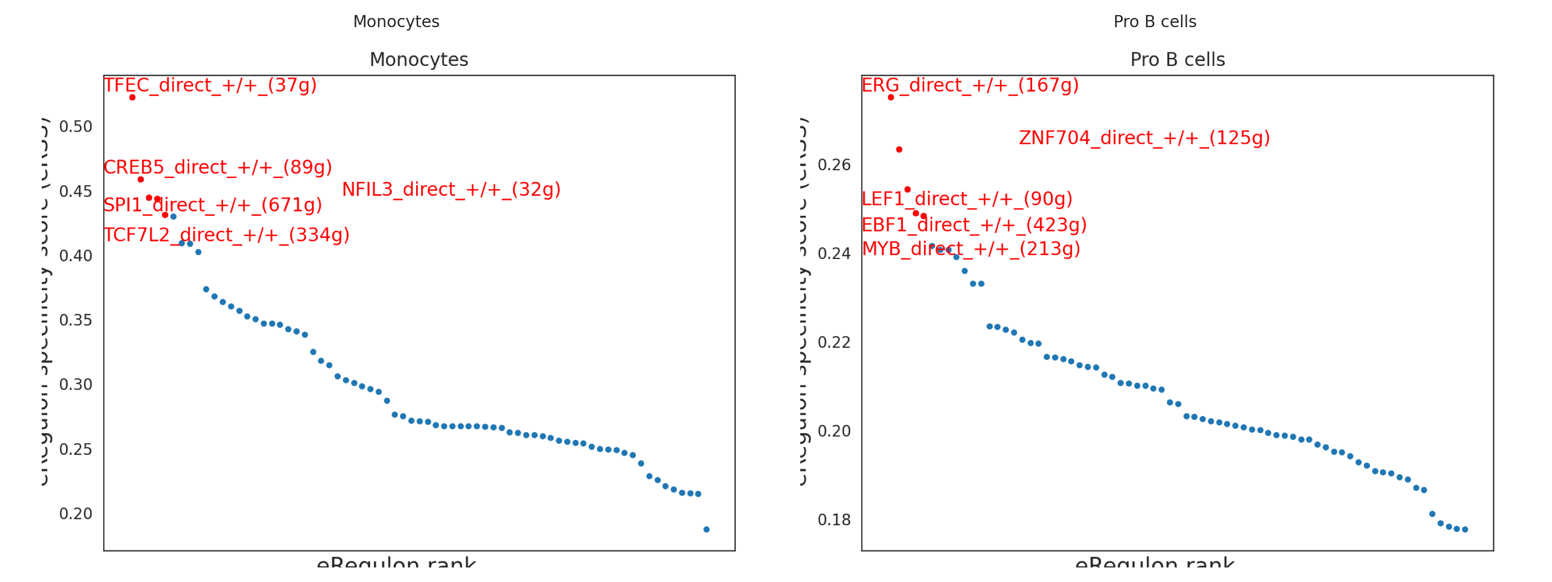
💡 Note:
- RSS Value Interpretation: The higher the RSS value, the stronger the specificity of the eRegulon in that cell type. Typically, the Top 5 RSS eRegulons represent the core regulators of that cell type.
- Multi-Modal Integration: Compute RSS using both direct and extended gene-based AUC matrices simultaneously, integrating both direct and indirect regulatory signals.
💡 Interpretation Guide
Global Description: The RSS plot displays the top eRegulons with the strongest activity in each cell type. The bar chart is arranged from high to low, with the leftmost bar being the most specific regulator for that cell type.
- Bar length: Represents the RSS score. The larger the value, the stronger the specificity.
- Cross-Cell-Type Comparison: If the same eRegulon appears only in a single cell type, it is a highly cell-type-specific regulator; if it appears across multiple cell types, it is likely a broad-spectrum regulator.
- Application Scenarios: Through RSS ranking, one can quickly identify the core transcription factors of each cell subpopulation, providing candidate targets for downstream functional validation.
7. eRegulon Dimensionality Reduction Visualization
7.1 Dimensionality Reduction Function Definition
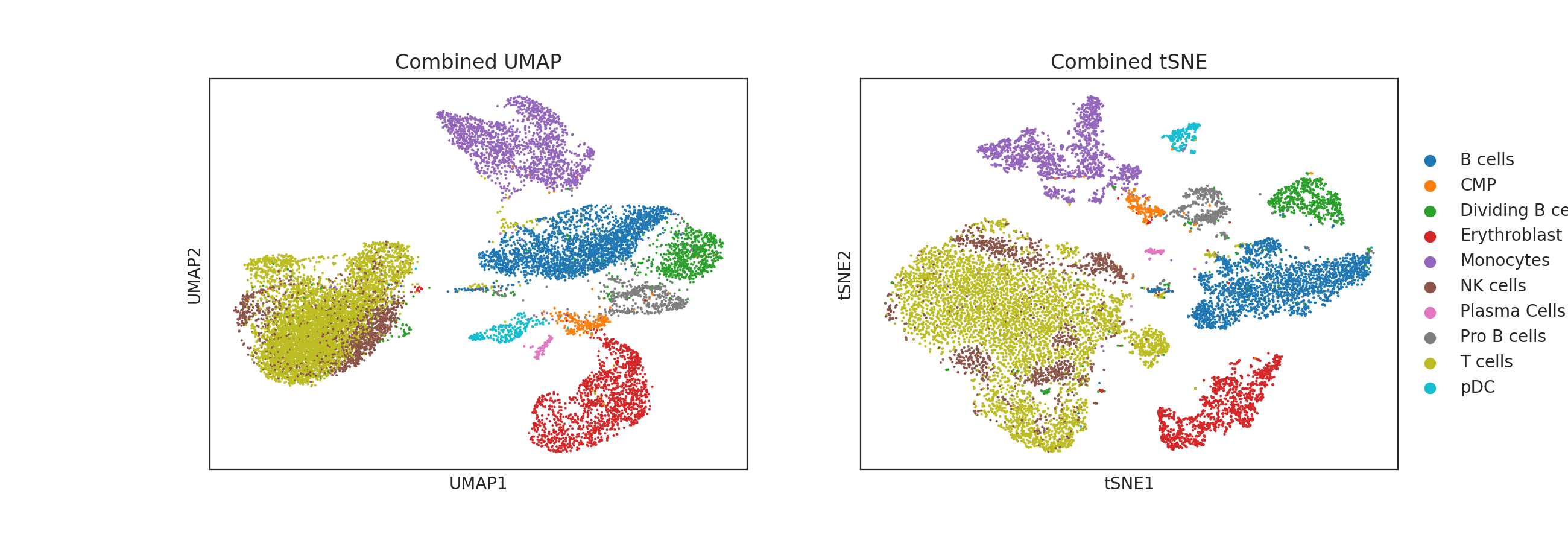
Perform UMAP/t-SNE dimensionality reduction based on the filtered eRegulon AUC matrix to display the distribution pattern of cells in the regulatory space. Unlike gene-expression-based dimensionality reduction, eRegulon dimensionality reduction directly reflects the cellular heterogeneity of regulatory activity.
Core Steps Breakdown:
- AUC Matrix Concatenation: Concatenate AUC matrices of the specified signature_keys (Gene-based / Region-based / both combined) column-wise to build a unified feature matrix.
- Metadata Alignment: Copy cell metadata (e.g., cell-type annotation) from the original MuData object into a temporary AnnData object, ensuring that dimensionality reduction results can be colored by cell type.
- PCA → Adjacency Graph → UMAP/t-SNE: First apply Z-score normalization to the AUC matrix, then perform PCA dimensionality reduction (
n_pcs), construct a KNN graph based on PCA results, and finally generate UMAP and/or t-SNE embeddings. - Result Saving: Save the dimensionality reduction coordinates back into the
scplus_obj.dr_celldictionary for subsequent visualization function calls.
import os
import pandas as pd
import matplotlib.pyplot as plt
import scanpy as sc
import anndata

def _run_dr(scplus_obj, mdata=None, methods=['umap', 'tsne'], scale=True,
            signature_keys=['Gene_based', 'Region_based'],
            suffix='', selected_regulons=None,
            n_pcs=50, random_state=0):
    auc_mats = []
    for k in signature_keys:
        df = scplus_obj.uns['eRegulon_AUC'][k].copy()
        if selected_regulons is not None:
            keep_cols = [c for c in df.columns if _eregulon_base_name(c) in [_eregulon_base_name(x) for x in selected_regulons]]
            df = df[keep_cols]
        auc_mats.append(df)

    merged_auc = pd.concat(auc_mats, axis=1)

    adata = anndata.AnnData(X=merged_auc.values)
    adata.obs_names = merged_auc.index
    adata.var_names = merged_auc.columns

    if mdata is not None:
        common_cells = adata.obs_names.intersection(mdata.obs_names)
        adata = adata[common_cells].copy()
        adata.obs = mdata.obs.loc[adata.obs_names].copy()
    elif hasattr(scplus_obj, 'metadata_cell'):
        common_cells = adata.obs_names.intersection(scplus_obj.metadata_cell.index)
        adata = adata[common_cells].copy()
        adata.obs = scplus_obj.metadata_cell.loc[adata.obs_names].copy()


    if scale:
        sc.pp.scale(adata)

    sc.tl.pca(adata, svd_solver='arpack', random_state=random_state)
    sc.pp.neighbors(adata, n_pcs=min(n_pcs, adata.obsm['X_pca'].shape[1]), random_state=random_state)


    if not hasattr(scplus_obj, 'dr_cell') or scplus_obj.dr_cell is None:
        scplus_obj.dr_cell = {}


    if 'umap' in methods:
        sc.tl.umap(adata, random_state=random_state)
        scplus_obj.dr_cell[f'eRegulons_UMAP{suffix}'] = adata.obsm['X_umap']
        print(f"[DR] Finished UMAP for {signature_keys}. Stored as eRegulons_UMAP{suffix}")

    if 'tsne' in methods:
        sc.tl.tsne(adata, random_state=random_state, use_rep='X_pca')
        scplus_obj.dr_cell[f'eRegulons_tSNE{suffix}'] = adata.obsm['X_tsne']
        print(f"[DR] Finished tSNE for {signature_keys}. Stored as eRegulons_tSNE{suffix}")

    return adata
7.2 Dimensionality Reduction Execution and Visualization
Core Steps Breakdown:
- Filter Condition Extraction: Retrieve the filtered eRegulon list from previous steps in
scplus_obj.uns. - Joint Dimensionality Reduction: Combine Gene-based and Region-based eRegulons to perform dimensionality reduction in a unified regulatory space. This joint approach captures cross-modal regulatory signals.
- Dual-Panel Visualization: Left panel shows UMAP (without legend to avoid occlusion); right panel shows t-SNE (legend retained). The same cell-type coloring scheme runs through both plots.
out_dir = "./result/eRegulon_reduction/"
os.makedirs(out_dir, exist_ok=True)

selected_gene_regulons = scplus_obj.uns['selected_eRegulons']['Gene_based']
selected_region_regulons = scplus_obj.uns['selected_eRegulons']['Region_based']
selected_regulons_combined = sorted(set(selected_gene_regulons) | set(selected_region_regulons))


# --- A. Gene-based Reduction ---
#adata_gene = _run_dr(scplus_obj,
#                     mdata=scplus_mdata,
#                     methods=['umap', 'tsne'],
#                     signature_keys=['Gene_based'],
#                     suffix='_gb',
#                     selected_regulons=selected_gene_regulons)

# --- B. Region-based Reduction ---
#adata_region = _run_dr(scplus_obj,
#                       mdata=scplus_mdata,
#                       methods=['umap', 'tsne'],
#                       signature_keys=['Region_based'],
#                       suffix='_rb',
#                       selected_regulons=selected_region_regulons)

# --- C. Combined (Gene + Region) Reduction ---

adata_combined = _run_dr(scplus_obj,
                         mdata=scplus_mdata,
                         methods=['umap', 'tsne'],
                         signature_keys=['Gene_based', 'Region_based'],
                         suffix='_combined',
                         selected_regulons=selected_regulons_combined)


def plot_and_save_reduction(adata, title_prefix, filename):
    fig, axes = plt.subplots(1, 2, figsize=(13, 4.5), constrained_layout=True)

    sc.pl.umap(adata, color=celltype_col_full, ax=axes[0],
               title=f"{title_prefix} UMAP", show=False, legend_loc=None)

    sc.pl.tsne(adata, color=celltype_col_full, ax=axes[1],
               title=f"{title_prefix} tSNE", show=False)

    fig.savefig(os.path.join(out_dir, filename), format="pdf", bbox_inches='tight')
    plt.show()
    plt.close(fig)


#plot_and_save_reduction(adata_gene, "Filtered Gene-based", "eRegulon_gene_AUC_reduction.pdf")
#plot_and_save_reduction(adata_region, "Filtered Region-based", "eRegulon_region_AUC_reduction.pdf")
plot_and_save_reduction(adata_combined, "Combined", "eRegulon_combined_AUC_reduction.pdf")[DR] Finished tSNE for ['Gene_based', 'Region_based']. Stored as eRegulons_tSNE_combined
/PROJ2/FLOAT/shumeng/apps/miniconda3/envs/scenicplus/lib/python3.11/site-packages/scanpy/plotting/_tools/scatterplots.py:378: UserWarning: No data for colormapping provided via 'c'. Parameters 'cmap' will be ignored
/PROJ2/FLOAT/shumeng/apps/miniconda3/envs/scenicplus/lib/python3.11/site-packages/scanpy/plotting/_tools/scatterplots.py:378: UserWarning: No data for colormapping provided via 'c'. Parameters 'cmap' will be ignored
降维与绘图全部完成,PDF 已保存!
8. Joint TF Expression and AUC UMAP Visualization
Map three signals — TF RNA expression, Gene-based AUC, and Region-based AUC — onto the same UMAP background, realizing a complete logical chain visualization from "regulatory initiation (TF expression) → chromatin changes (Region AUC) → gene expression (Gene AUC)."
Core Steps Breakdown:
- Axis Orientation Detection: Automatically determine the gene/cell axis orientation of the
X_EXPmatrix (row vs column), compatible with storage formats from different data sources. - Name Mapping: Precisely match the TF portion of eRegulon names with gene names in X_EXP, and simultaneously establish the mapping tables for Gene/Region AUC column names.
- Top eRegulon Selection: For each cell type, select the Top 5 eRegulons with the highest RSS as visualization targets.
- Expression Smoothing: When the maximum TF expression value > 50, apply log1p smoothing to compress the impact of extremely high expression values on color distribution.
- UMAP Mapping: Map the three signals — TF expression, Gene-based AUC, Region-based AUC — separately onto three-panel UMAP plots, using
vmax="p99"to truncate the top 1% extreme values, ensuring optimal visualization of moderate expression specificity.
💡 Note:
- log1p Smoothing: Single-cell RNA expression data often contain extreme high-expression values; log1p transformation compresses the dynamic range, making the color gradient more uniform.
- p99 Truncation: Setting the UMAP legend upper limit to the 99th percentile prevents a few extreme cells from skewing the entire color scale.
Use the Combined dimensionality reduction (_run_dr output) as the unified background to plot:
- TF expression, 2) TF-corresponding Gene-based AUC, 3) TF-corresponding Region-based AUC
import os
import numpy as np
import matplotlib.pyplot as plt
import scanpy as sc


if not hasattr(scplus_obj, "X_EXP"):
    raise AttributeError("scplus_obj lacks X_EXP, cannot extract TF expression.")

exp_df = scplus_obj.X_EXP
if not hasattr(exp_df, "index") or not hasattr(exp_df, "columns"):
    raise TypeError("scplus_obj.X_EXP is not a table structure indexed by genes and cells.")

umap_out_dir = "./result/TF_AUC_Combined_UMAP/"
os.makedirs(umap_out_dir, exist_ok=True)


adata_cells = set(adata_combined.obs_names.astype(str))
idx_names = exp_df.index.astype(str)
col_names = exp_df.columns.astype(str)
idx_cell_hits = len(adata_cells.intersection(set(idx_names)))
col_cell_hits = len(adata_cells.intersection(set(col_names)))


if idx_cell_hits >= col_cell_hits:
    exp_cells_axis = "index"
    exp_genes_axis = "columns"
    exp_cell_names = exp_df.index
    exp_gene_names = exp_df.columns
else:
    exp_cells_axis = "columns"
    exp_genes_axis = "index"
    exp_cell_names = exp_df.columns
    exp_gene_names = exp_df.index

print(f"[EXP] detected cells on {exp_cells_axis}, genes on {exp_genes_axis}")

exp_gene_map = {}
for g in exp_gene_names.astype(str):
    exp_gene_map.setdefault(g.lower(), g)

gene_var_map = {}
for v in eRegulon_gene_AUC.var_names.astype(str):
    gene_var_map.setdefault(_eregulon_base_name(v), v)

region_var_map = {}
for v in eRegulon_region_AUC.var_names.astype(str):
    region_var_map.setdefault(_eregulon_base_name(v), v)

def _to_1d_array(x):
    if hasattr(x, "toarray"):
        return x.toarray().ravel()
    if hasattr(x, "todense"):
        return np.asarray(x.todense()).ravel()
    return np.asarray(x).ravel()

common_cells = (
    adata_combined.obs_names
    .intersection(eRegulon_gene_AUC.obs_names)
    .intersection(eRegulon_region_AUC.obs_names)
    .intersection(exp_cell_names)
)

for ct in rss.index:
    top5_eregulons = rss.loc[ct].sort_values(ascending=False).head(5).index.tolist()
    for ereg in top5_eregulons:
        tf_name = str(ereg).split("_")[0]
        matched_tf = exp_gene_map.get(tf_name.lower())
        gene_col = gene_var_map.get(_eregulon_base_name(str(ereg)))
        region_col = region_var_map.get(_eregulon_base_name(str(ereg)))

        if not matched_tf:
            print(f"Warning: TF {tf_name} not found in RNA matrix.")
            continue
        if gene_col is None or region_col is None:
            print(f"Warning: regulon {ereg} not found in gene/region AUC matrices.")
            continue

        plot_adata = adata_combined[common_cells].copy()


        if exp_genes_axis == "index":
            expr_vals = _to_1d_array(exp_df.loc[matched_tf, common_cells].values)
        else:
            expr_vals = _to_1d_array(exp_df.loc[common_cells, matched_tf].values)

        if np.max(expr_vals) > 50:
            expr_vals = np.log1p(expr_vals)

        gene_auc_vals = _to_1d_array(eRegulon_gene_AUC[common_cells, gene_col].X)
        region_auc_vals = _to_1d_array(eRegulon_region_AUC[common_cells, region_col].X)

        expr_key = f"{tf_name}__expr"
        gene_key = f"{tf_name}__gene_auc"
        region_key = f"{tf_name}__region_auc"

        plot_adata.obs[expr_key] = expr_vals
        plot_adata.obs[gene_key] = gene_auc_vals
        plot_adata.obs[region_key] = region_auc_vals

        fig, axes = plt.subplots(1, 3, figsize=(15, 4.5))
        sc.pl.umap(plot_adata, color=expr_key, cmap="viridis", vmax="p99", show=False, ax=axes[0], title=f"{tf_name} Expression")
        sc.pl.umap(plot_adata, color=gene_key, cmap="viridis", vmax="p99", show=False, ax=axes[1], title=f"{tf_name} Gene-based AUC")
        sc.pl.umap(plot_adata, color=region_key, cmap="viridis", vmax="p99", show=False, ax=axes[2], title=f"{tf_name} Region-based AUC")

        safe_ereg = str(ereg).replace("/", "_").replace("+", "pos").replace("-", "neg")
        safe_ct = str(ct).replace("/", "_").replace(" ", "_")
        pdf_path = os.path.join(umap_out_dir, f"{safe_ct}_combined_umap_{safe_ereg}.pdf")
        fig.savefig(pdf_path, bbox_inches="tight")
        plt.close(fig)

print(f"Combined UMAP plots saved to {os.path.abspath(umap_out_dir)}")if last_fig is not None:
display(last_fig)
print(f"Show the last plot: {pdf_path}")
else:
print("no pictures")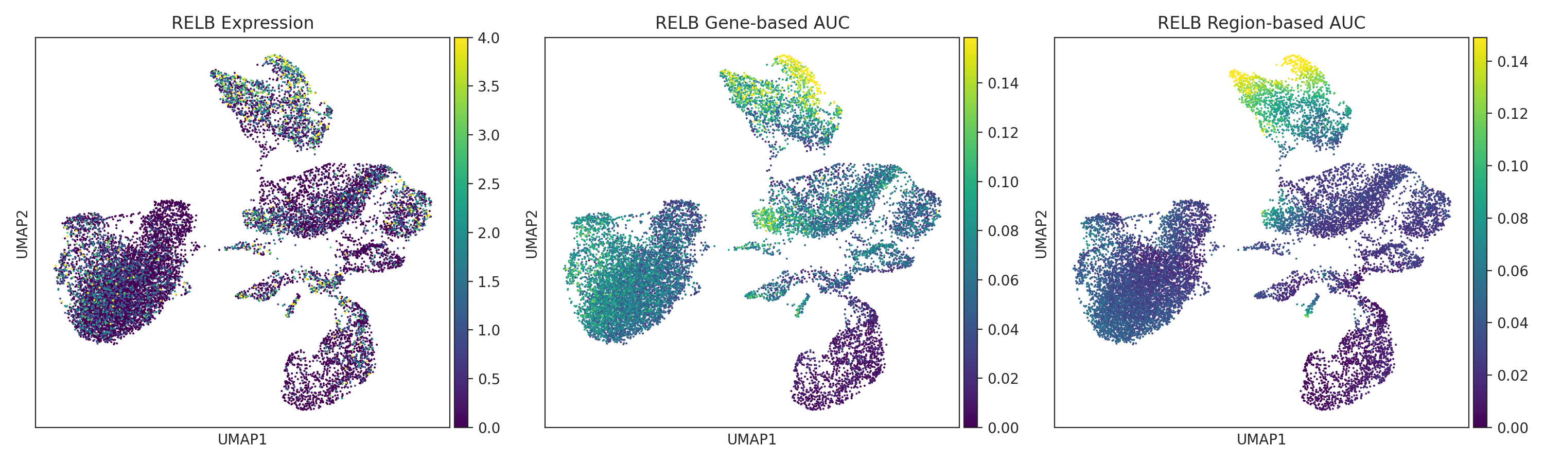
展示最后一张图: ./result/TF_AUC_Combined_UMAP/Plasma_Cells_combined_umap_RELB_direct_pos_pos_(69g).pdf
💡 Note:
- Gene-based vs Region-based: Gene-based dimensionality reduction reflects cell grouping based on target gene expression patterns; Region-based dimensionality reduction reflects grouping based on chromatin accessibility patterns.
- Combined Dimensionality Reduction: Uses both AUC matrices simultaneously, capturing the most comprehensive regulatory heterogeneity signal — recommended as the primary analysis result.
- Commented Code: Standalone Gene-based and Region-based dimensionality reduction code has been commented out. To enable, simply uncomment the corresponding lines.
9. Joint Heatmap–Dotplot Visualization
9.1 SCENIC+ Built-in heatmap_dotplot
Using SCENIC+'s built-in heatmap_dotplot function, represent Region-based AUC by dot size and Gene-based AUC by color, simultaneously displaying the regulatory activity of both modalities in a single figure.
Core Steps Breakdown:
- Metadata Filtering: Retain only regulons that pass filtering on both Gene and Region sides, ensuring that only high-quality eRegulons are displayed in the dotplot.
- Dual-Channel Encoding: The color channel (Gene-based AUC) reflects regulatory activity at the target gene expression level; the dot-size channel (Region-based AUC) reflects regulatory activity at the chromatin accessibility level.
- Horizontal Layout: eRegulons are arranged by row, cell types by column, facilitating inspection of each eRegulon's cell-type-specific pattern.
from scenicplus.plotting.dotplot import heatmap_dotplotavail_gene = set(scplus_mdata_filt.mod["direct_gene_based_AUC"].var_names.astype(str))
avail_region = set(scplus_mdata_filt.mod["direct_region_based_AUC"].var_names.astype(str))
meta = scplus_mdata_filt.uns["direct_e_regulon_metadata"].copy()
meta = meta[
meta["Gene_signature_name"].astype(str).isin(avail_gene) &
meta["Region_signature_name"].astype(str).isin(avail_region)
].copy()
subset_names = meta["eRegulon_name"].astype(str).unique().tolist()
plot = heatmap_dotplot(
scplus_mudata=scplus_mdata_filt,
color_modality="direct_gene_based_AUC",
size_modality="direct_region_based_AUC",
group_variable=celltype_col_full,
eRegulon_metadata_key="direct_e_regulon_metadata",
color_feature_key="Gene_signature_name",
size_feature_key="Region_signature_name",
feature_name_key="eRegulon_name",
subset_feature_names=subset_names,
sort_data_by="direct_gene_based_AUC",
orientation="horizontal",
figsize=(19, 8)
)
plot = plot + theme(
axis_text_x=element_text(
# rotation=90,
# hjust=0.5,
# vjust=0.5,
angle=90,
size=12
# color='black',
# margin={'t': 10},
# va='top'
),
axis_text_y=element_text(size=12),
legend_position = 'bottom'
)
dotplot_out_dir = "./result/Regulon_Specificity_Score/"
os.makedirs(dotplot_out_dir, exist_ok=True)
dotplot_pdf = os.path.join(dotplot_out_dir, "direct_eRegulon_heatmap_dotplot.pdf")
plot.save(dotplot_pdf, format="pdf", width=19, height=8, units="in", verbose=False)
print(f"Heatmap-dotplot has been saved: {dotplot_pdf}")plot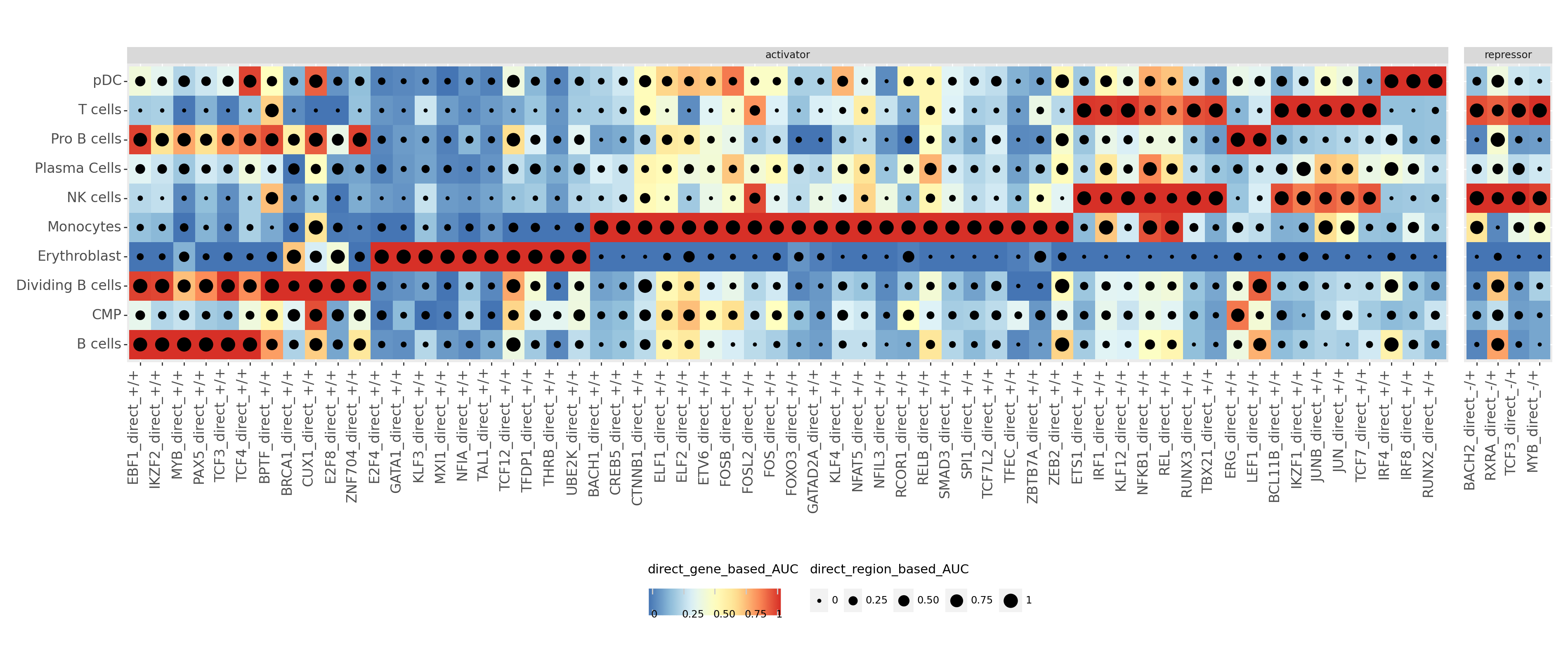
<Figure Size: (1900 x 800)>
9.2 Custom RSS–Expression Joint Dotplot
Building on the preceding SCENIC+ built-in dotplot, further construct a custom joint dotplot using color to represent TF expression Z-score and dot size to represent RSS score, achieving dual-dimensional visualization of regulatory activity (RSS) and expression level (Z-score).
Core Steps Breakdown:
- Top TF Extraction: Extract the Top N (default 6) eRegulons from each cell type's RSS matrix as visualization targets.
- Expression Extraction and Normalization: Extract expression of the corresponding TF from the RNA modality, compute mean by cell-type group, then apply Z-score normalization (clipped to [-2, 2]) to eliminate absolute dimensional differences.
- Dynamic Threshold: Use the 5th percentile of RSS as threshold, filtering out low-specificity eRegulon–cell-type combinations to avoid overcrowding the plot.
- Joint Encoding: Background color blocks represent TF expression Z-score (red = high expression, blue = low expression); black dot size represents RSS score, achieving precise alignment of dual-modal signals on the same plot.
import pandas as pd
import numpy as np
from plotnine import *
from sklearn.preprocessing import StandardScaler

print("Building custom RSS and Expression dotplot...")

group_var = celltype_col_full
top_n = 6

rna_keys = [k for k in scplus_mdata.mod.keys() if 'RNA' in k.upper() or 'GEX' in k.upper()]
if not rna_keys:
   raise ValueError("Cannot find RNA/GEX modality in scplus_mdata")
rna_key = rna_keys[0]
adata_rna = scplus_mdata.mod[rna_key]

adata_rna.obs[group_var] = scplus_mdata.obs[group_var].values

selected_regulons = []
for ct in rss.index:
   selected_regulons.extend(rss.loc[ct].sort_values(ascending=False).head(top_n).index.tolist())
selected_regulons = list(dict.fromkeys(selected_regulons))


plot_data = []
celltypes = rss.index.tolist()

for reg in selected_regulons:
   tf_name = reg.split('_')[0]

   if tf_name in adata_rna.var_names:
       if hasattr(adata_rna[:, tf_name].X, 'todense'):
           expr_array = np.ravel(adata_rna[:, tf_name].X.todense())
       else:
           expr_array = np.ravel(adata_rna[:, tf_name].X)

       df_tmp = pd.DataFrame({'expr': expr_array, 'group': adata_rna.obs[group_var].values})
       mean_expr = df_tmp.groupby('group')['expr'].mean().reindex(celltypes).fillna(0)
   else:
       mean_expr = pd.Series(0, index=celltypes)

   z_expr = StandardScaler().fit_transform(mean_expr.values.reshape(-1, 1)).flatten()
   z_expr = np.clip(z_expr, -2, 2)

   for i, ct in enumerate(celltypes):
       plot_data.append({
           'CellType': ct,
           'eRegulon': reg,
           'RSS': rss.loc[ct, reg],
           'Expression_Zscore': z_expr[i]
       })

df_plot = pd.DataFrame(plot_data)


rss_60th = np.percentile(df_plot['RSS'], 5)
rss_max = df_plot['RSS'].max()
print(f"Calculated 60th percentile for RSS: {rss_60th:.4f}")
print(f"Calculated Maximum RSS: {rss_max:.4f}")

df_plot['RSS_plot'] = df_plot['RSS'].where(df_plot['RSS'] >= rss_60th, np.nan)


df_plot['CellType'] = pd.Categorical(df_plot['CellType'], categories=celltypes[::-1], ordered=True)
df_plot['eRegulon'] = pd.Categorical(df_plot['eRegulon'], categories=selected_regulons, ordered=True)


custom_plot = (
   ggplot(df_plot, aes(x='eRegulon', y='CellType'))
   + geom_tile(aes(fill='Expression_Zscore'), color='white', size=0.5)
   + scale_fill_cmap(cmap_name='RdYlBu_r', limits=(-2, 2))
   + geom_point(aes(size='RSS_plot'), color='black', na_rm=True)
   + scale_size_continuous(range=(1.5, 6), limits=(rss_60th, rss_max))
   + theme_minimal()
   + theme(
       axis_text_x=element_text(angle=90, hjust=1, vjust=1, size=10),
       axis_text_y=element_text(size=10),
       panel_grid_major=element_blank(),
       figure_size=(max(8, len(selected_regulons)*0.3), max(6, len(celltypes)*0.5))
   )
   + labs(x='', y='', fill='Expression\n(Z-score)', size='RSS')
)


dotplot_out_dir = "./result/Regulon_Specificity_Score/"
os.makedirs(dotplot_out_dir, exist_ok=True)
dotplot_pdf = os.path.join(dotplot_out_dir, "RSS_expersion_heatmap_dotplot.pdf")
custom_plot.save(dotplot_pdf, format="pdf", width=19, height=8, units="in", verbose=False)
print(f"Heatmap-dotplot has been saved: {dotplot_pdf}")Calculated Maximum RSS: 0.6351
Heatmap-dotplot 已保存: ./result/Regulon_Specificity_Score/RSS_expersion_heatmap_dotplot.pdf
custom_plot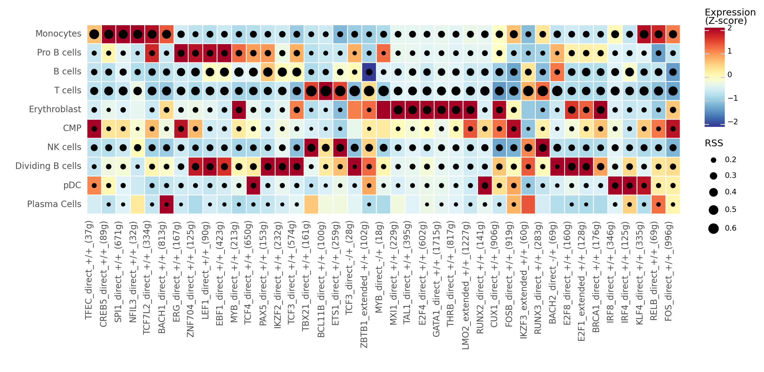
<Figure Size: (1230 x 600)>
💡 Interpretation Guide
Global Description: The custom dotplot integrates the RSS score (dot size) and TF expression level (color) into a single matrix. Each row represents a cell type; each column represents an eRegulon.
- Color gradient: Red indicates the TF is highly expressed in that cell type; blue indicates low expression. Z-score > 0 means expression above the global average.
- Dot size: Larger dots indicate higher RSS scores, i.e., stronger specificity of that eRegulon to that cell type.
- Empty cells (no dots): Indicate that the eRegulon's RSS in that cell type falls below the percentile threshold, with non-significant specificity.
- Joint Interpretation: An ideal cell-type-specific regulator should simultaneously satisfy "large dot + red" — i.e., high RSS specificity and high expression level. If the dot is large but the color is bluish, this may suggest post-transcriptional regulatory mechanisms.
10. Saving Analysis Results
Serialize the scplus_obj object — containing all analysis results (filtered eRegulons, dimensionality reduction coordinates, metadata, etc.) — into a pickle file for reuse in subsequent analyses.
💡 Note:
- Use
dillrather than standardpickle, becausedillcan serialize more complex Python objects (e.g., lambda functions, nested classes, etc.).- The serialized object can be reloaded via
dill.load(), with alluns,dr_cell,X_EXP, and other attributes fully preserved.
Use a raw string; no f-string needed.
import dill

pkl_file = "./scplus_obj.pkl"
with open(pkl_file, 'wb') as f:
    dill.dump(scplus_obj, f)
11. List of Prerequisite Files for the Complete Pipeline
Listed in dependency order:
Step 0: Seurat → AnnData Conversion
| File | Description | Source |
|---|---|---|
*.rds | Seurat object, must contain both RNA and ATAC assays | User-provided data |
meta.tsv (optional) | External metadata table, TSV format, first column is cell barcode, must contain the column specified by celltype_col, plus orig.ident and Sample columns | User-provided |
Step 1: pycisTopic Topic Modeling
| File | Description | Source |
|---|---|---|
scATAC.h5ad | ATAC AnnData output from Step 0 (automatically read, no extra preparation needed) | step0 output |
{species}-blacklist.v2.bed | ENCODE blacklist BED file (selected by species: mouse/human/fly/chicken/rat) | Download in advance, provided by Aertslab |
Step 2: cisTarget Custom Database Construction
| File | Description | Source |
|---|---|---|
consensus_regions.bed | Region BED output from Step 1 (automatically read) | step1 output |
genome.fa + genome.fa.fai | Reference genome FASTA + index (selected by species) | Download in advance |
{species}.chrom.sizes | Chromosome size file (mm10/hg38/dm6/GRCg7b/rn7) | Download in advance |
*.cb file collection | Aertslab motif collection (all .cb files under v10nr_clust_public/singletons/ directory) | Download in advance, from SCENIC/AERTSLAB |
cbust executable | Cluster Buster motif scanning tool | Compile/download in advance |
create_fasta_with_padded_bg_from_bed.sh | Helper script (invoked from bin/create_cisTarget_databases/) | Included in the repository |
create_cistarget_motif_databases.py | Helper script (invoked from bin/create_cisTarget_databases/) | Included in the repository |
Step 3: SCENIC+ Pipeline Core Inference
| File | Description | Source |
|---|---|---|
scRNA.h5ad | RNA AnnData output from Step 0 | step0 output |
cistopic_obj_with_models.pkl | CistopicObject output from Step 1 | step1 output |
binarized_topics.pkl | Binarized topics output from Step 1 | step1 output |
{species}_custom.*.rankings.feather | Rankings database output from Step 2 | step2 output |
{species}_custom.*.scores.feather | Scores database output from Step 2 | step2 output |
motifs-v10-nr.*.tbl | Motif annotation table (under snapshots directory, selected by species) | Included in the motif collection |
genes.gtf | GTF genome annotation file (used to generate genome_annotation.tsv) | Download in advance, selected by species |
{assembly}.chrom.sizes | Same as step2, needs to be placed in the data/ directory | Same as step2 |
Step 4: Post-Processing (notebook)
| File | Description | Source |
|---|---|---|
scplusmdata.h5mu | Final MuData output from Step 3 pipeline | step3 output |
ctx_results.hdf5 | cisTarget enrichment results | step3 output |
dem_results.hdf5 | Differential accessibility results | step3 output |
Databases/Reference Files to Download and Prepare in Advance (6 Categories)
| # | File Type | Species Coverage | Download Source |
|---|---|---|---|
| 1 | Reference Genome FASTA | mouse (mm10), human (hg38), fly, chicken, rat | UCSC / Ensembl |
| 2 | Chromosome Size File (.chrom.sizes) | Same species | UCSC Genome Browser |
| 3 | GTF Genome Annotation File | Same species (must contain gene_name/gene_id, gene_type fields) | Ensembl / GENCODE / CellRanger ARC |
| 4 | ENCODE Blacklist (.blacklist.v2.bed) | mouse, human, fly, etc. | ENCODE Project |
| 5 | Aertslab motif collection (incl. singletons/.cb + snapshots/.tbl) | Cross-species (v10nr_clust) | SCENIC AERTSLAB |
| 6 | cbust executable | Universal | AERTSLAB Cluster Buster |
Items 1–4 are one per species; items 5–6 are shared across the entire project.