ATAC + RNA Multi-omics: Single-Sample Analysis Based on Signac

Author: SeekGene

Time: 29 min

Words: 5.8k words

Updated: 2026-07-07

Reads: 0 times

1. Tutorial Overview

This tutorial is built on the Seurat + Signac single-cell multi-omics analysis toolkit and is designed to perform single-sample fundamental analysis, joint dimensionality reduction and clustering, and cell-type annotation on the SeekArc single-cell multi-omics data (RNA + ATAC). It further carries out differential peak analysis, LinkPeaks analysis, Motif analysis, and Footprint analysis.

This pipeline is intended for single-cell datasets where each cell simultaneously carries transcriptomic expression information and chromatin accessibility information. Within a single sample, it integrates the RNA and ATAC modalities to deliver a complete workflow — from data loading and quality control through joint analysis and regulatory mechanism dissection — achieving the following core analytical objectives:

• Single-Sample Multi-Omics Joint Analysis: Simultaneously leveraging RNA expression and ATAC open-chromatin information within the same sample to more comprehensively characterize cellular states and biological heterogeneity.
• Data Quality Control and Preprocessing: Performing quality control, normalization, and dimensionality reduction separately on the RNA and ATAC modalities to provide a reliable data foundation for downstream analyses.
• Single-Modality and Multi-Modality Clustering: Carrying out RNA clustering, ATAC clustering, and joint clustering based on WNN (Weighted Nearest Neighbor), respectively, for comparing cell grouping results across different modalities.
• Joint Dimensionality Reduction and Visualization: Fusing RNA and ATAC modality information to construct a more stable low-dimensional representation, and displaying cell distribution patterns via UMAP.
• Cell-Type Annotation: Providing biological interpretation and cell-type labeling of clustering results by combining marker gene expression patterns.
• Differential Peaks Analysis: Identifying differentially accessible chromatin regions across cell groups or conditions, and screening for regulatory elements associated with cellular states.
• Differential Peaks Annotation: Annotating differential peaks with their nearest genes to aid interpretation of their potential regulatory functions.
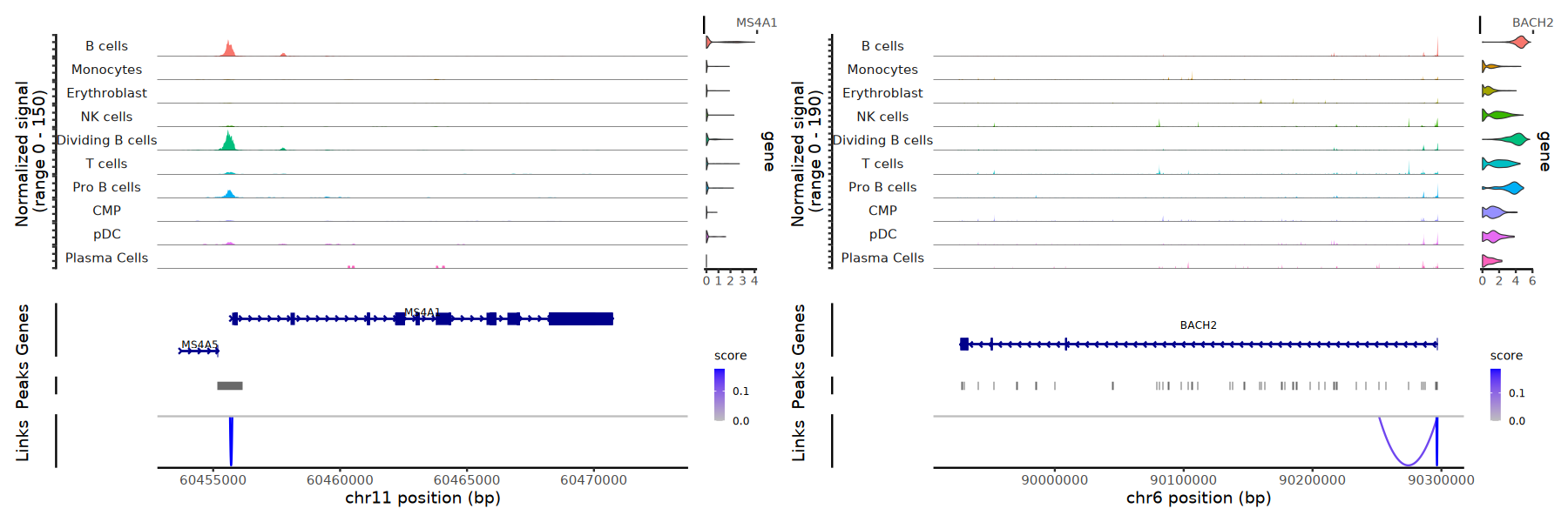
• LinkPeaks Analysis: Linking chromatin accessibility peaks to target gene expression to identify putative regulatory relationships, and validating them visually using gene-region accessibility.
• Motif Enrichment Analysis: Performing transcription factor binding site enrichment analysis on differentially accessible peaks, to screen for key transcription factors potentially involved in cellular-state regulation.
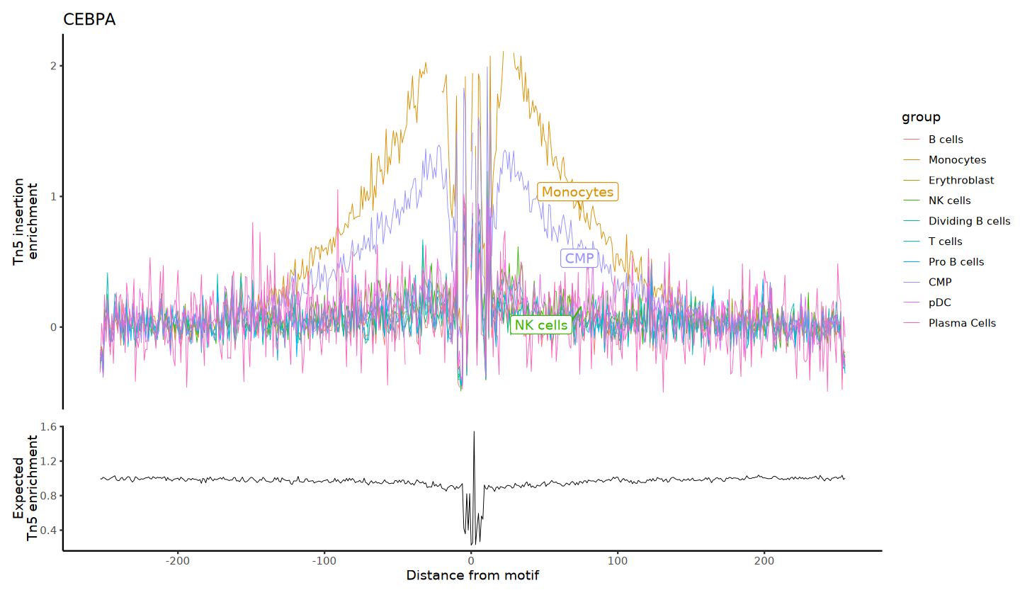
• Footprint Analysis: By inspecting the "footprint" signal formed by protein binding around transcription factor binding sites (motifs), precisely evaluating the actual binding activity of specific transcription factors, thereby deeply dissecting the cell-type-specific gene regulatory networks across different cell types.

#加载必要的R包
suppressPackageStartupMessages({
  library(Seurat)
  library(Signac)
  library(EnsDb.Hsapiens.v86)
  library(BSgenome.Hsapiens.UCSC.hg38)
  library(biovizBase)
  #library(BSgenome.Mmusculus.UCSC.mm10)
  #library(EnsDb.Mmusculus.v79)
  library(JASPAR2020)
  library(TFBSTools)
  library(dplyr)
  library(ggplot2)
  library(patchwork)
  library(harmony)
})

set.seed(1234)

options(future.globals.maxSize = 8000 * 1024^2)  # 8GB

my36colors <-c( '#E5D2DD', '#53A85F', '#F1BB72', '#F3B1A0', '#D6E7A3', '#57C3F3', '#476D87',
                '#E95C59', '#E59CC4', '#AB3282', '#23452F', '#BD956A', '#8C549C', '#585658',
                '#9FA3A8', '#E0D4CA', '#5F3D69', '#C5DEBA', '#58A4C3', '#E4C755', '#F7F398',
                '#AA9A59', '#E63863', '#E39A35', '#C1E6F3', '#6778AE', '#91D0BE', '#B53E2B',
                '#712820', '#DCC1DD', '#CCE0F5', '#CCC9E6', '#625D9E', '#68A180', '#3A6963',
                '#968175', "#6495ED", "#FFC1C1",'#f1ac9d','#f06966','#dee2d1','#6abe83','#39BAE8','#B9EDF8','#221a12',
                '#b8d00a','#74828F','#96C0CE','#E95D22','#017890')

2. Input File Preparation

2.1 Input File Requirements

Single-sample analysis requires that the RNA expression matrix, ATAC peak accessibility matrix, and corresponding fragment files be organized under the same sample directory. The sample folder is recommended to be named directly with the sample ID, for example S127. This directory should contain the following:

• filtered_feature_bc_matrix: scRNA-seq expression matrix directory, containing barcodes.tsv.gz, features.tsv.gz, and matrix.mtx.gz.
• filtered_peaks_bc_matrix: scATAC-seq peak accessibility matrix directory, containing barcodes.tsv.gz, features.tsv.gz, and matrix.mtx.gz.
• {sampleID}_A_fragments.tsv.gz: ATAC fragment file, used for downstream construction of ChromatinAssay, computation of TSS enrichment, nucleosome signal, and related analyses.
• {sampleID}_A_fragments.tsv.gz.tbi: Index file corresponding to the ATAC fragment file.

2.2 Example Directory Structure

S127/
├── filtered_feature_bc_matrix/
│   ├── barcodes.tsv.gz
│   ├── features.tsv.gz
│   └── matrix.mtx.gz
├── filtered_peaks_bc_matrix/
│   ├── barcodes.tsv.gz
│   ├── features.tsv.gz
│   └── matrix.mtx.gz
├── S127_A_fragments.tsv.gz
└── S127_A_fragments.tsv.gz.tbi

2.3 Notes

• Input files must be placed under the same sample directory with a correct path structure; otherwise, this tutorial may fail to read them.
• The ATAC fragment file and its index file must exist as a pair; otherwise, ChromatinAssay cannot be constructed properly.
• RNA and ATAC data should come from the same batch of cells or the same multi-omics experimental system to ensure accuracy of downstream joint analyses.
• ATAC peak coordinate format must be consistent with the chromosome naming style of the reference genome annotation.

---

3. Data Loading and Preprocessing

Before commencing the single-sample multi-omics analysis, the genome annotation must be loaded, and the RNA and ATAC data for a single sample must be read and used to build the analysis object.

3.1 Obtaining Gene Annotation Information

First, read the reference genome annotation from the EnsDb database and generate an annotation object. This annotation contains gene positions, transcription start sites (TSS), and other information, which can be used for downstream TSS enrichment analysis, gene activity analysis, and peak annotation.

This example uses the human annotation database EnsDb.Hsapiens.v86, unifies chromosome names to the format with the chr prefix, and specifies the reference genome version as hg38. This ensures consistency between the annotation and the chromosome naming in the ATAC data, avoiding errors in downstream analyses.

suppressWarnings({
  suppressMessages({
    annotation <- GetGRangesFromEnsDb(ensdb = EnsDb.Hsapiens.v86)
    seqlevels(annotation) <- paste0('chr', seqlevels(annotation))
    genome(annotation) <- 'hg38'
  })
})

3.2 Data Reading and Object Construction

Read the single-sample RNA expression matrix, ATAC peak accessibility matrix, and fragment file, and construct a Seurat object containing dual-omics information.

This step mainly includes the following:

1. Reading RNA Data: Read the scRNA-seq expression matrix from the filtered_feature_bc_matrix directory and create a Seurat object for the RNA assay.
2. Reading ATAC Data: Read the scATAC-seq peak accessibility matrix from the filtered_peaks_bc_matrix directory, while specifying the fragment file path.
3. Constructing the ATAC Assay: Use CreateChromatinAssay() to create the ATAC assay, incorporating the previously generated annotation to support downstream TSS enrichment analysis, peak annotation, and other ATAC analyses.
4. Building the Multi-Omics Object: Add the ATAC assay to the existing RNA Seurat object, obtaining a single-sample multi-omics object that contains both RNA and ATAC information.

Upon completion of this step, a standard single-sample SeekArc multi-omics Seurat object is obtained, ready for downstream quality control, normalization, dimensionality reduction, clustering, and cell-type annotation.

# --- Input Parameter Configuration ---
file_path = "/path/to/sampleDir/"
sample_name = "pbmc_1"

atac_path <- file.path(file_path, sample_name, 'filtered_peaks_bc_matrix')
rna_path <- file.path(file_path, sample_name, 'filtered_feature_bc_matrix')
frag_path <- file.path(file_path, sample_name, paste0(sample_name, '_A_fragments.tsv.gz'))

rna_counts <- Read10X(data.dir = rna_path)
# create a Seurat object containing the RNA adata
seu <- CreateSeuratObject(
  counts = rna_counts,
  assay = "RNA"
)

atac_counts <- Read10X(data.dir = atac_path)
atac_counts <- atac_counts[Matrix::rowSums(atac_counts > 0) >= 3, ]  
# create ATAC assay and add it to the object
seu[["ATAC"]] <- CreateChromatinAssay(
  counts = atac_counts,
  sep = c(":", "-"),
  fragments = frag_path,
  annotation = annotation
)

4. Data Quality Control

4.1 Quality Metric Computation

Before starting the analysis, quality control must be performed to remove low-quality cells and ensure the reliability of downstream results. This step computes commonly used quality metrics for both RNA and ATAC modalities.

RNA Quality Metrics:

• percent.mt: Proportion of mitochondrial genes, typically used to assess cell status; abnormally high values may indicate low-quality or damaged cells.

ATAC Quality Metrics:

• TSS.enrichment: TSS enrichment score, evaluating the degree to which open-chromatin signal is enriched around transcription start sites.
• nucleosome_signal: Nucleosome signal, reflecting fragment distribution characteristics; generally, lower is better.
• nCount_ATAC: Total ATAC count per cell, measuring chromatin accessibility signal intensity.
• nFeature_RNA: Number of RNA features detected per cell, assisting in cell quality assessment.

suppressWarnings({
  suppressMessages({
          seu[["percent.mt"]] <- PercentageFeatureSet(seu, pattern = "^MT-")
          DefaultAssay(seu) <- "ATAC"
          seu <- TSSEnrichment(object = seu, fast = FALSE) 
          seu <- NucleosomeSignal(object = seu)
  })
})

Note: The quality metrics for seekARC dual-omics data also include nCount_RNA, nCount_ATAC, nFeature_RNA, nFeature_ATAC, and others, which are automatically generated during Seurat object construction in the preceding step.

4.2 Quality Metric Visualization

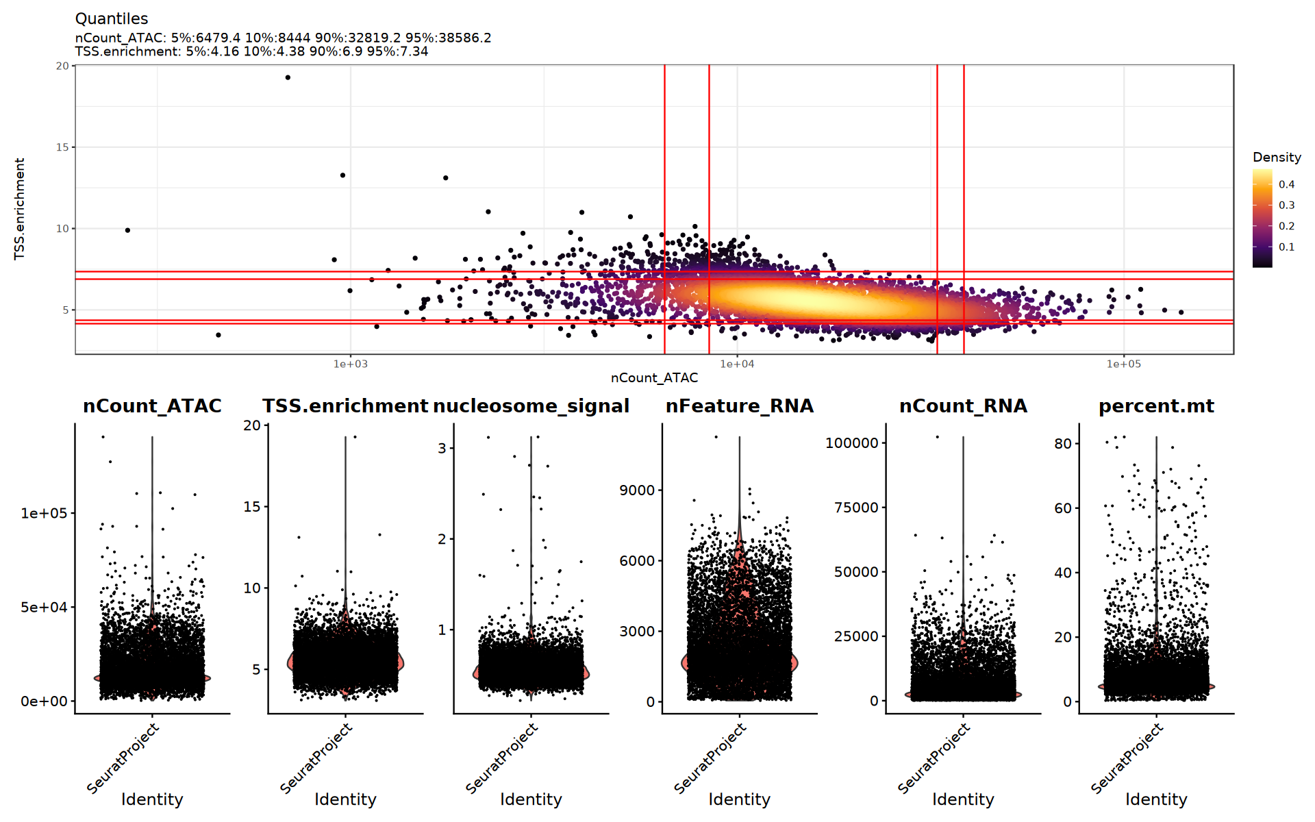
After computing the quality metrics, violin plots and scatter plots can be used to inspect the distribution of each metric, helping to assess data quality and select appropriate filtering thresholds.

It is recommended to focus on the following:

• Whether there are obvious outliers, long-tailed distributions, or bimodal distributions;
• Whether the distributions of quality metrics are consistent across different samples;
• Reasonable adjustment of filtering thresholds based on the visualization results, to obtain clearer downstream clustering and UMAP results.

options(repr.plot.width = 16, repr.plot.height = 10)
suppressWarnings({
  p1=DensityScatter(seu, x = 'nCount_ATAC', y = 'TSS.enrichment', log_x = TRUE, quantiles = TRUE)
  p2=VlnPlot(
      object = seu,
      features = c('nCount_ATAC', 'TSS.enrichment',  'nucleosome_signal',"nFeature_RNA", "nCount_RNA", "percent.mt"),
      pt.size = 0.1,
      ncol = 6
  )
 print(p1 / p2)
})

4.3 Filtering Out Low-Quality Cells

Based on the quality metrics computed above, low-quality cells are filtered out to remove abnormal cells and improve the reliability of downstream analysis results. Specific filtering thresholds should be set according to the actual sample conditions, typically guided by the violin plots and scatter plots of the quality metrics.

cells_before <- ncol(seu)
  
seu <- subset(seu,
    subset = nFeature_RNA > 200 &
             nFeature_RNA < 8000 &
             nCount_RNA > 500 &
             nCount_RNA < 30000 &
             percent.mt < 20 &
             nCount_ATAC > 500 &
             nCount_ATAC < 50000 &
             TSS.enrichment > 1 &
             nucleosome_signal < 1
  )
  
cells_after <- ncol(seu)

5. Data Normalization

5.1 RNA Data Normalization and Linear Dimensionality Reduction

After quality control and low-quality cell filtering, RNA data must be normalized and reduced in dimension to provide a basis for downstream clustering analysis. This includes:

1. Data Normalization: Using Seurat's default LogNormalize method to normalize each cell's expression values and apply a log transformation, reducing the impact of differences in sequencing depth.
2. Highly Variable Gene Selection: Selecting genes that show high variability across cells, to be used in downstream dimensionality reduction and clustering.
3. Data Scaling: Applying a linear transformation to the gene expression matrix so that different genes become comparable, preparing the data for PCA.
4. PCA Dimensionality Reduction: Performing Principal Component Analysis (PCA) on the normalized RNA data to extract the major sources of variation, used for downstream neighbor search, clustering, and visualization.

suppressWarnings({
  suppressMessages({
      DefaultAssay(seu) <- "RNA"
      seu <- NormalizeData(seu, assay = "RNA")
      seu <- FindVariableFeatures(seu, assay = "RNA", selection.method = "vst", nfeatures = 2000)
      seu <- ScaleData(seu, assay = "RNA")
      seu <- RunPCA(seu, assay = "RNA", npcs = 50)
      })
    })

5.2 ATAC Data Normalization and Linear Dimensionality Reduction

After RNA data preprocessing, ATAC data also require normalization and dimensionality reduction to extract chromatin accessibility features and provide a basis for downstream clustering and joint analysis. This includes:

1. Data Normalization: Using the TF-IDF method provided by Signac to normalize ATAC data, correcting for differences in sequencing depth across cells and enhancing the detection of rare peaks.
2. Feature Selection: Using FindTopFeatures() to select peak features for downstream analysis, typically retaining peaks with strong signals or those present in a certain number of cells.
3. SVD Dimensionality Reduction: Performing Singular Value Decomposition (SVD) on the normalized ATAC matrix to extract the major sources of variation, used for downstream neighbor search, clustering, and joint analysis.

suppressWarnings({
  suppressMessages({
      seu <- RunTFIDF(seu, assay = "ATAC")
      seu <- FindTopFeatures(seu, assay = "ATAC", min.cutoff = 'q0')
      seu <- RunSVD(seu, assay = "ATAC")
  })
})

6. Nonlinear Dimensionality Reduction and Clustering Analysis

Having completed the normalization and linear dimensionality reduction of RNA and ATAC data, we can further reveal the complex relationships of cells in high-dimensional space using nonlinear dimensionality reduction methods. Commonly used nonlinear techniques include t-SNE and UMAP, which map high-dimensional data into two- or three-dimensional space to facilitate visualization of cell subpopulation structure.

Three Clustering Strategies

1. RNA Clustering: Based on gene expression similarity, constructing a nearest-neighbor graph using the PCA results of the RNA-seq data.
2. ATAC Clustering: Based on chromatin accessibility similarity, constructing a nearest-neighbor graph using the LSI results of the ATAC-seq data.
3. WNN Clustering: Integrating both modalities (recommended), based on the weighted nearest neighbor algorithm, comprehensively considering the contributions of RNA and ATAC modalities to cell similarity.

Note:

Before performing dimensionality reduction and clustering, the optimal number of dimensions for both RNA and ATAC data must be determined separately to avoid noise interference or information loss.

options(repr.plot.width = 13, repr.plot.height = 7)
DepthCor(seu, reduction = "lsi",n = 50)

💡 NoteLSI Dimension Selection: In ATAC data analysis, the first LSI component sometimes more strongly reflects technical factors such as sequencing depth rather than biological variation. Therefore, it is recommended to use DepthCor() to evaluate the correlation between each LSI dimension and sequencing depth. If the first dimension is found to be strongly correlated with sequencing depth, it is typically excluded from downstream neighbor search, UMAP dimensionality reduction, and clustering analyses. (The second dimension may occasionally behave similarly.)

ElbowPlot(seu, ndims =30, reduction = "pca")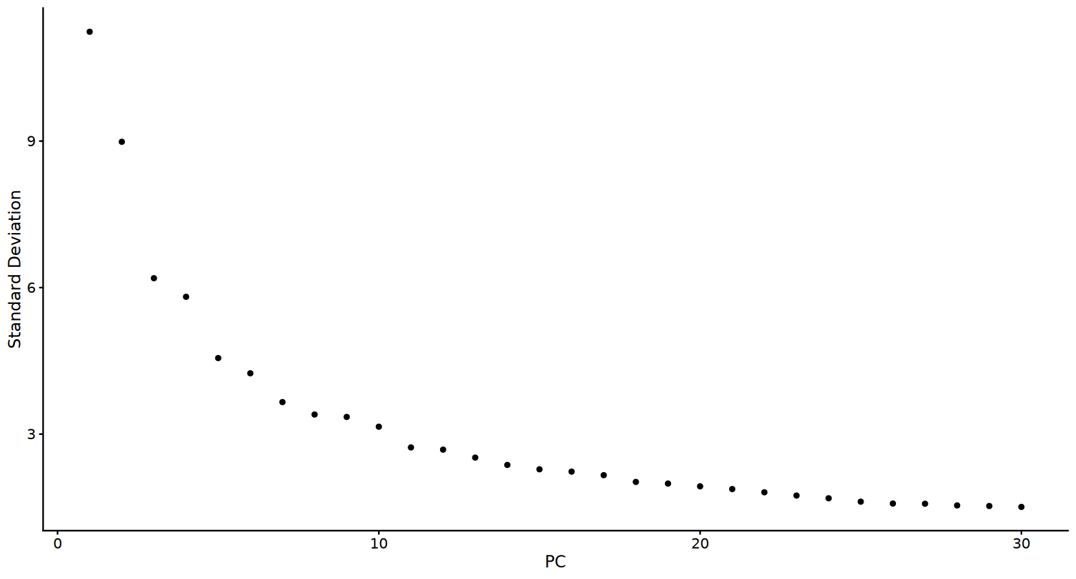

💡 NotePrincipal Component Dimension Selection: In RNA data analysis, ElbowPlot() can be used to inspect how much of the overall variation each principal component explains, thereby assisting in deciding the number of dimensions to retain for downstream analysis. Typically, after an obvious "elbow" in the curve, the contribution of additional principal components to variation gradually weakens, so the region around that elbow serves as a reference range for dimension truncation. Note that the true dimensionality of the data rarely has an absolute fixed threshold; it is recommended to combine the elbow plot, known biological information, and downstream results for a comprehensive decision. In practice, one may try different dimension numbers within adjacent ranges, such as 10, 15, or higher, and prefer a slightly larger dimension range to avoid missing potential biological signals.

6.1 WNN Joint Dimensionality Reduction and Clustering

After determining the effective dimensions of PCA and LSI, dimensionality reduction and clustering analysis can begin.

suppressWarnings({
  suppressMessages({
      seu <- FindMultiModalNeighbors(seu, reduction.list = list("pca", "lsi"), dims.list = list(1:30, 3:30))

      seu <- FindClusters(seu, graph.name = "wknn", resolution = 0.5)

      seu <- RunUMAP(seu, nn.name = "weighted.nn", reduction.name = "wnn.umap")
        })
})

output

Modularity Optimizer version 1.3.0 by Ludo Waltman and Nees Jan van Eck

Number of nodes: 7515
Number of edges: 108882

Running Louvain algorithm...n Maximum modularity in 10 random starts: 0.9158
Number of communities: 13
Elapsed time: 0 seconds

options(repr.plot.width = 9, repr.plot.height = 7)
DimPlot(seu, reduction = "wnn.umap", group.by = "wknn_res.0.5",label=T, cols = my36colors) + ggtitle("WNN")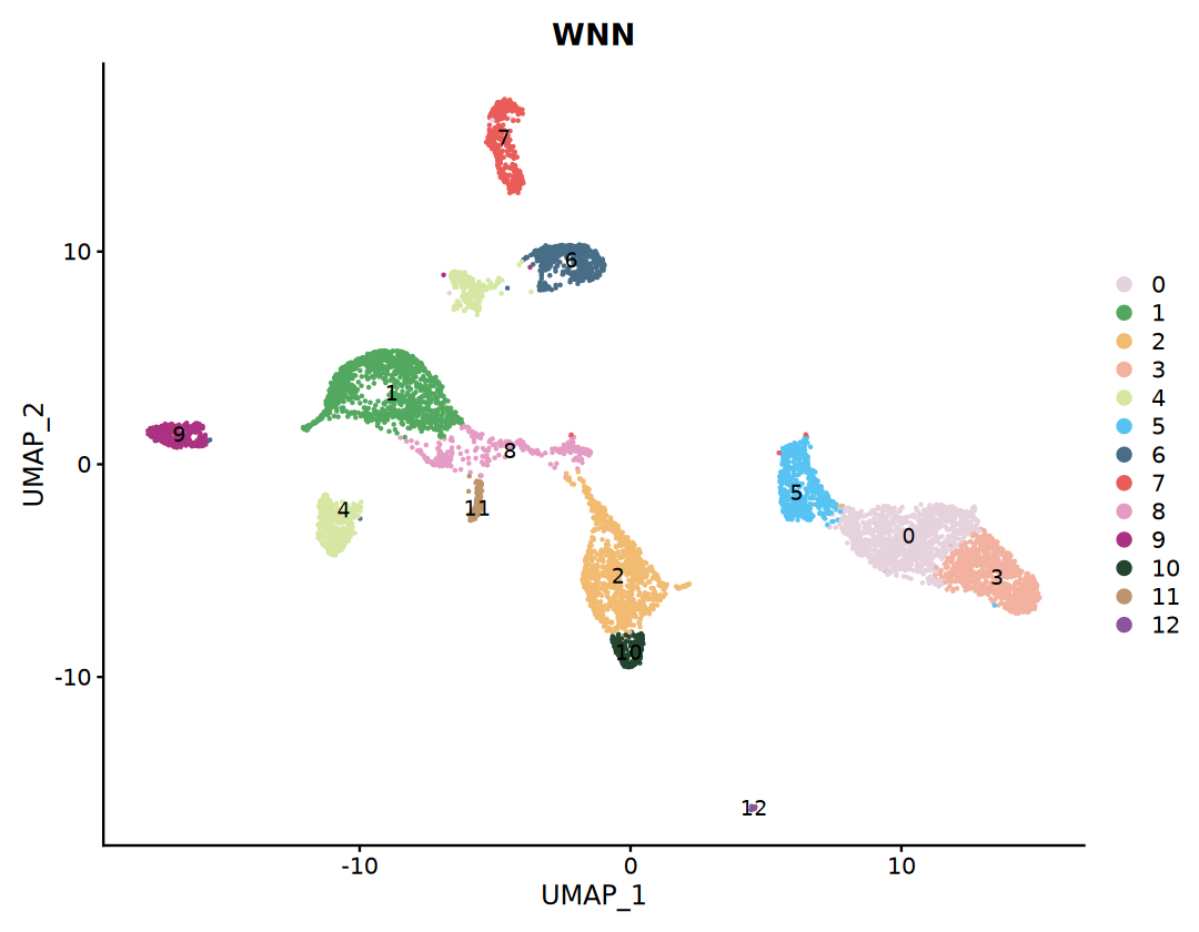

6.2 Dimensionality Reduction and Clustering Based on RNA Data

suppressWarnings({
  suppressMessages({
      seu <- RunUMAP(seu, reduction = "pca", dims = 1:30, assay = "RNA",reduction.name="rnaumap")
      seu <- FindNeighbors(seu, reduction = "pca", dims = 1:30, assay = "RNA",graph.name = "rnaneigobr")
      seu <- FindClusters(seu, resolution = 0.5, algorithm = 1,graph.name = "rnaneigobr")
        })
})

output

Modularity Optimizer version 1.3.0 by Ludo Waltman and Nees Jan van Eck

Number of nodes: 7515
Number of edges: 71144

Running Louvain algorithm...n Maximum modularity in 10 random starts: 0.9152
Number of communities: 23
Elapsed time: 0 seconds

DimPlot(seu, reduction = "rnaumap", group.by = "rnaneigobr_res.0.5",label=T, cols = my36colors) + ggtitle("RNA")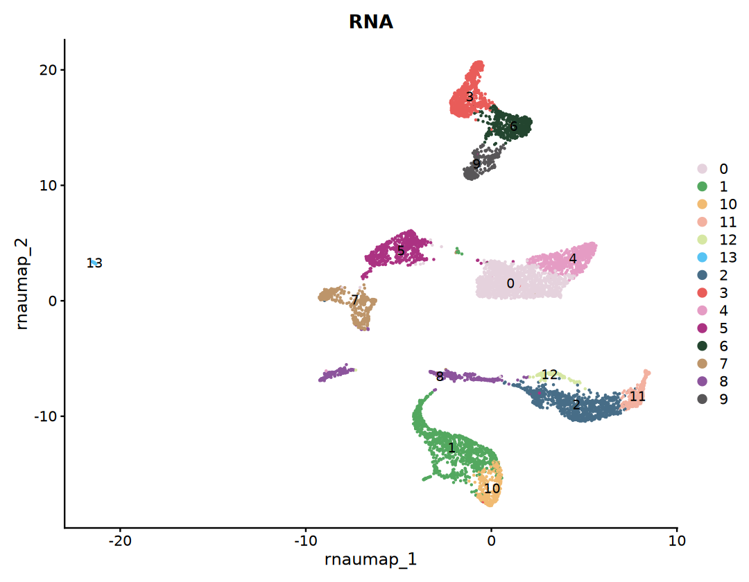

6.3 Dimensionality Reduction and Clustering Based on ATAC Data

suppressWarnings({
  suppressMessages({
      seu <- RunUMAP(seu, reduction = "lsi", dims = 1:30, assay = "ATAC",reduction.name="atacumap")
      seu <- FindNeighbors(seu, reduction = "lsi", dims = 1:30, assay = "ATAC",graph.name = "atacneigobr")
      seu <- FindClusters(seu, resolution = 0.5, algorithm = 1,graph.name = "atacneigobr")
        })
})

output

Modularity Optimizer version 1.3.0 by Ludo Waltman and Nees Jan van Eck

Number of nodes: 7515
Number of edges: 70618

Running Louvain algorithm...n Maximum modularity in 10 random starts: 0.9129
Number of communities: 15
Elapsed time: 0 seconds

DimPlot(seu, reduction = "atacumap", group.by = "atacneigobr_res.0.5",label=T, cols = my36colors) + ggtitle("ATAC")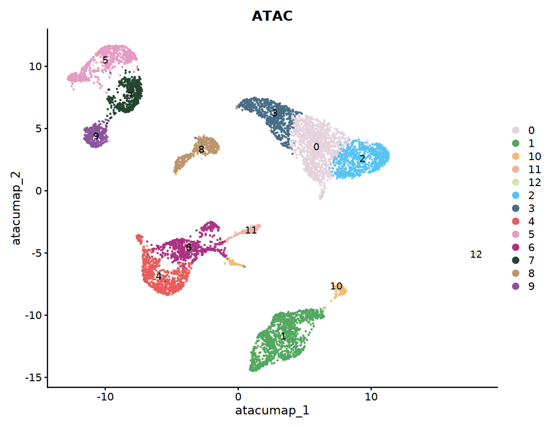

💡 NoteNote: Different methods may yield different clustering results; WNN clustering typically can discover finer cell subpopulations. It is recommended to prioritize WNN results for cell annotation and downstream analyses.

7. Cell-Type Annotation

7.1 Differentially Expressed Gene Selection

Identify genes that are specifically highly expressed in each cluster, and screen for representative marker genes based on expression proportion and fold change, providing a preliminary basis for cell-type identification. A bubble plot can be used to inspect the expression of top differentially expressed genes across clusters, assisting in determining the cell type corresponding to each cluster.

Idents(seu) <- seu@meta.data$wknn_res.0.5
pbmc.markers <- FindAllMarkers(seu, only.pos = TRUE, min.pct = 0.25, logfc.threshold = 0.58)

head(pbmc.markers)

A data.frame: 6 × 7

	p_val	avg_log2FC	pct.1	pct.2	p_val_adj	cluster	gene
	<dbl>	<dbl>	<dbl>	<dbl>	<dbl>	<fct>	<chr>
ACSM3	0	2.909427	0.861	0.272	0	0	ACSM3
RUBCNL	0	2.567519	0.937	0.379	0	0	RUBCNL
ROR1	0	2.547254	0.779	0.193	0	0	ROR1
RAPGEF5	0	2.422696	0.874	0.290	0	0	RAPGEF5
PCDH9	0	2.418539	0.883	0.416	0	0	PCDH9
DTX1	0	2.367083	0.879	0.254	0	0	DTX1

top.pbmc.markers <- pbmc.markers %>% 
group_by(cluster) %>% 
  top_n(n = 3, wt = avg_log2FC)

options(repr.plot.width=12, repr.plot.height=6)


DefaultAssay(seu)="RNA"
pbmc.markers <- pbmc.markers[!duplicated(pbmc.markers$gene),]
DotPlot(seu, 
        group.by = "wknn_res.0.5", 
        features = unique(top.pbmc.markers$gene),
        cols = c("#f8f8f8","#ff3472"),
        #dot.min = 0.05,
        
        dot.scale = 8)+ 
  #RotatedAxis() + 
  scale_x_discrete("") + 
  scale_y_discrete("") +
  theme(
    axis.text.x = element_text(size = 12, face = "bold", 
                              angle = 45, hjust = 1, vjust = 1),
    axis.text.y = element_text(size = 12, face = "bold"),
    plot.title = element_text(size = 14, face = "bold", hjust = 0.5),
    legend.title = element_text(size = 10, face = "bold")
  ) +
  ggtitle("Top DEG Genes Expression") +
  labs(color = "Expression\nLevel")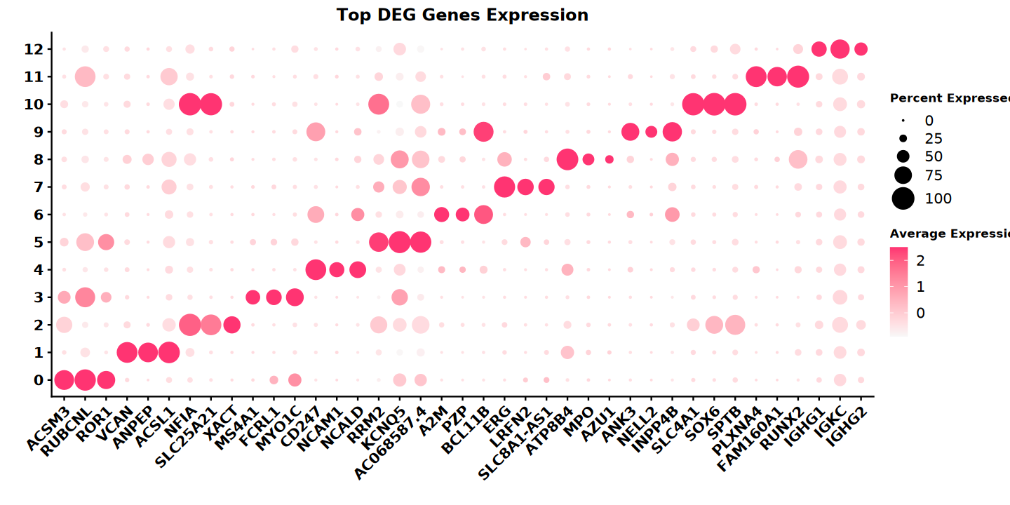

7.2 Inspecting Marker Gene Expression at the scRNA-seq Data Level

Using classical marker genes of known cell types, verify the biological attributes of each cluster at the RNA expression level to achieve preliminary cell-type matching. The example data in this tutorial are PBMC, so we have compiled common immune cell types and their corresponding marker gene sets. In actual analyses, the marker genes should be customized according to sample origin and tissue type.

pbmc_marker_classic <- list(
  "Plasma Cells" = c("IGHG1", "IGKC"),
  "Monocytes" = c("VCAN", "FCN1", "TREM1"),
  "B cells" = c("MS4A1", "BACH2", "PAX5"),
  "CMP" = c("MPO"),
  "Pro B cells" = c("DNTT"),
  "Erythroblast" = c("ALAS2", "NFIA", "SOX6"),
  "T cells" = c("PLXNA4", "THEMIS", "ITK", "BCL11B"),
  "NK cells" = c("NCAM1", "KLRC3"),
  "Dividing B cells" = c("MKI67", "TOP2A"),
  "pDC" = c("RUNX2")
)

Single-cell dual-omics data annotation is generally based on WNN multi-modal dimensionality reduction clustering results, with annotation performed according to marker gene expression patterns in the WNN clustering output.

options(repr.plot.width=12, repr.plot.height=6)

DefaultAssay(seu)="RNA"
DotPlot(seu, 
        group.by = "wknn_res.0.5", 
        features = pbmc_marker_classic,
        cols = c("#f8f8f8","#ff3472"),
       #dot.min = 0.05,
       dot.scale = 8)+  
  RotatedAxis() + 
  scale_x_discrete("") + 
  scale_y_discrete("") +
  theme(
    axis.text.x = element_text(size = 12, face = "bold", 
                              angle = 45, hjust = 1, vjust = 1),
    axis.text.y = element_text(size = 12, face = "bold"),
    plot.title = element_text(size = 14, face = "bold", hjust = 0.5),
    legend.title = element_text(size = 10, face = "bold")
  ) +
  ggtitle("Marker Genes Expression") +
  labs(color = "Expression\nLevel")

output

Warning message:
"The \`facets\` argument of \`facet_grid()\` is deprecated as of ggplot2 2.2.0.
ℹ Please use the \`rows\` argument instead.
ℹ The deprecated feature was likely used in the Seurat package.
Please report the issue at ."

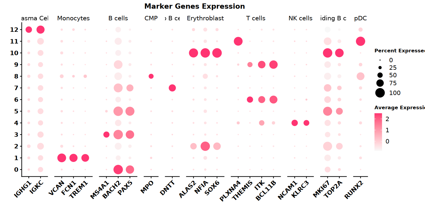
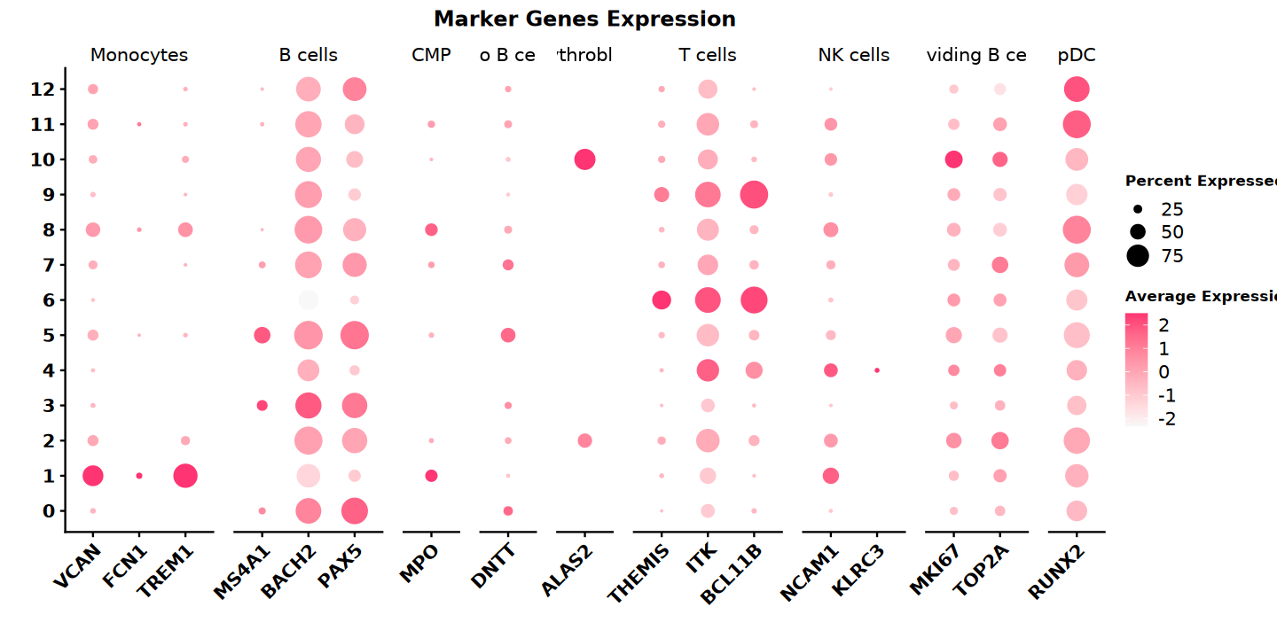
💡 NoteNote: ① The bubble color reflects the gene's average expression level in the subpopulation (light color → low expression, dark color → high expression); ② The bubble size represents the proportion of cells expressing that gene. The horizontal axis labels represent marker genes; the top labels indicate which cell type each corresponding marker gene belongs to.

7.3 Evaluating Marker Gene Activity via Chromatin Accessibility

Using ATAC-seq data, compute the chromatin accessibility activity of the same marker genes, validating the RNA expression-based annotation results from the epigenetic layer and improving the accuracy of cell-type identification.

DefaultAssay(seu) <- "ATAC"
pbmc_marker_genes <- unlist(pbmc_marker_classic, use.names = FALSE)
gene.activities <- GeneActivity(seu,features = pbmc_marker_genes)

# add the gene activity matrix to the Seurat object as a new assay and normalize it
seu[['GeneActivity']] <- CreateAssayObject(counts = gene.activities)
seu <- NormalizeData(
  object = seu,
  assay = 'GeneActivity',
  normalization.method = 'LogNormalize',
  scale.factor = median(seu$nCount_GeneActivity)
)

DefaultAssay(seu)="GeneActivity"
existing_genes <- rownames(seu)

pbmc_marker_classic <- lapply(pbmc_marker_classic, function(gene_vec) {
  gene_vec[gene_vec %in% existing_genes]
})

pbmc_marker_classic <- pbmc_marker_classic[sapply(pbmc_marker_classic, length) > 0]

options(repr.plot.width=12, repr.plot.height=6)

DotPlot(seu, 
        group.by = "wknn_res.0.5", 
        features = pbmc_marker_classic,
        cols = c("#f8f8f8","#ff3472"),
       dot.min = 0.05,
       dot.scale = 8)+  
  RotatedAxis() + 
  scale_x_discrete("") + 
  scale_y_discrete("") +
  theme(
    axis.text.x = element_text(size = 12, face = "bold", 
                              angle = 45, hjust = 1, vjust = 1),
    axis.text.y = element_text(size = 12, face = "bold"),
    plot.title = element_text(size = 14, face = "bold", hjust = 0.5),
    legend.title = element_text(size = 10, face = "bold")
  ) +
  ggtitle("Marker Genes Expression") +
  labs(color = "Expression\nLevel")

output

Warning message:
"Removed 50 rows containing missing values or values outside the scale range
(\`geom_point()\`)."

7.4 Accessibility of Marker Gene Genomic Regions

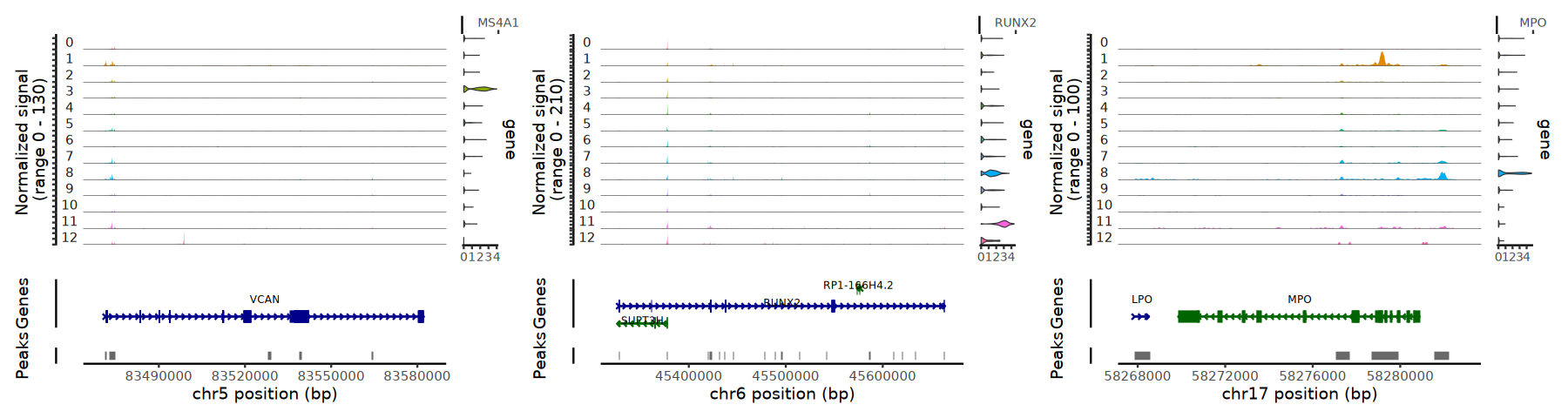
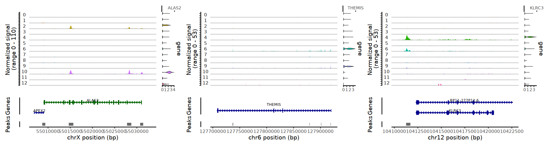
Using CoveragePlot, simultaneously display the chromatin accessibility pattern and RNA expression level of specific marker genes, visually validating the consistency between the two omics data on genomic coordinates, and providing visualization evidence for cell-type-specific marker expression and accessibility.

DefaultAssay(seu) <- "ATAC"
P1 <- CoveragePlot(
  object = seu,
  region = "VCAN",
  features = "MS4A1",
  expression.assay = "RNA",
  extend.upstream = 2000,
  extend.downstream = 2000
)

P2 <- CoveragePlot(
  object = seu,
  region = "RUNX2",
  features = "RUNX2",
  expression.assay = "RNA",
  extend.upstream = 2000,
  extend.downstream = 2000
)

P3 <- CoveragePlot(
  object = seu,
  region = "MPO",
  features = "MPO",
  expression.assay = "RNA",
  extend.upstream = 2000,
  extend.downstream = 2000
)

P4 <- CoveragePlot(
  object = seu,
  region = "ALAS2",
  features = "ALAS2",
  expression.assay = "RNA",
  extend.upstream = 2000,
  extend.downstream = 2000
)

P5 <- CoveragePlot(
  object = seu,
  region = "THEMIS",
  features = "THEMIS",
  expression.assay = "RNA",
  extend.upstream = 2000,
  extend.downstream = 2000
)

P6 <- CoveragePlot(
  object = seu,
  region = "KLRC3",
  features = "KLRC3",
  expression.assay = "RNA",
  extend.upstream = 2000,
  extend.downstream = 2000
)

options(repr.plot.width=15, repr.plot.height=4)
patchwork::wrap_plots(P1, P2, P3, ncol = 3)
patchwork::wrap_plots(P4, P5, P6, ncol = 3)

output

Warning message:
"Removed 54 rows containing missing values or values outside the scale range
(\`geom_segment()\`)."

Warning message:
"Removed 90 rows containing missing values or values outside the scale range
(\`geom_segment()\`)."

Warning message:
"Removed 11 rows containing missing values or values outside the scale range
(\`geom_segment()\`)."

Warning message:
"Removed 3 rows containing missing values or values outside the scale range
(\`geom_segment()\`)."

8. Cell Annotation

8.1 Cell-Type Annotation

Integrating the multi-omics analysis results of differentially expressed gene screening, classical marker gene expression patterns, and chromatin accessibility activity, systematically identify the cell type of each cluster obtained from WNN clustering. By establishing a mapping between cluster IDs and known cell types (e.g., B cells, T cells, monocytes, NK cells, etc.), biological classification of all cells is completed.

celltype_mapping <- c(
  "12" = "Plasma Cells",
  "1" = "Monocytes",
  "0" = "B cells",
  "3" = "B cells",
  "8" = "CMP",
  "7" = "Pro B cells",
  "2" = "Erythroblast",
  "6" = "T cells",
  "4" = "NK cells",
  "5" = "Dividing B cells",
  "11" = "pDC",
  "9" = "T cells",
  "10" = "Erythroblast"
)

seu$celltype <- recode(
  seu$wknn_res.0.5,
  !!!celltype_mapping
)

output

开始细胞类型注释... 1780451715

8.2 Annotation Result Visualization

Visualize the cell-type annotation results in the WNN-UMAP dimensionality-reduction space, intuitively displaying the distribution patterns of different cell types in two-dimensional space, validating the rationality of the annotations and the separation effectiveness of the cell populations.

p1 <- DimPlot(
  seu,
  reduction = "wnn.umap",
  group.by = "celltype",
  label = TRUE,
  label.size = 3,
  cols = my36colors
) +
  ggtitle("celltype") +
  theme(legend.position = "bottom")

options(repr.plot.width=9, repr.plot.height=8)
print(p1)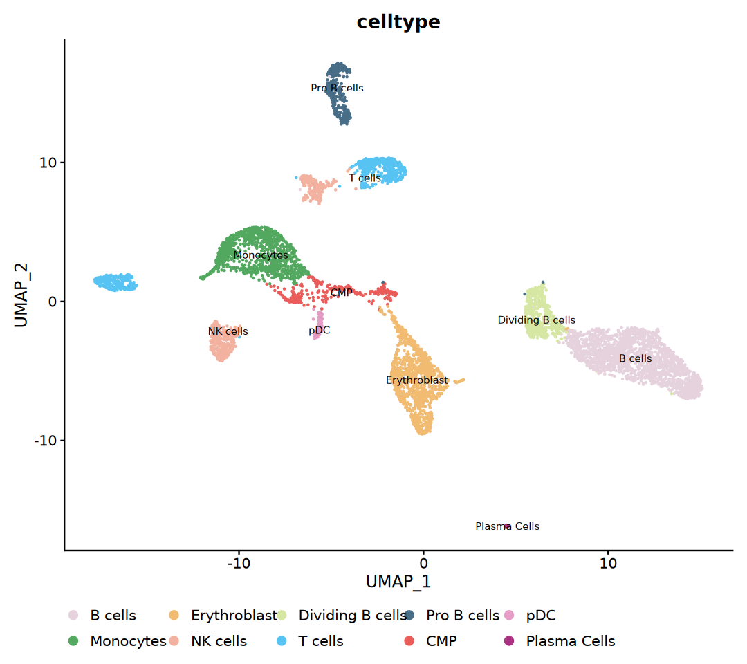

output

细胞类型注释可视化...

9. Advanced Analyses

9.1 Differential Peak Analysis

To identify cell-type-specific regulatory sequences, perform enrichment analysis in chromatin regions that are differentially accessible between cell types. For sparse data (scATAC-seq), it is usually necessary to appropriately lower the min.pct threshold in FindMarkers().

Idents(seu) <- "celltype"
DefaultAssay(seu) <- "ATAC"
da_peaks <- FindMarkers(
  object = seu,
  ident.1 = 'B cells',
  ident.2 = 'T cells',
  only.pos = TRUE,
  test.use = 'LR',
  min.pct = 0.1,
  logfc.threshold = 0.58
)

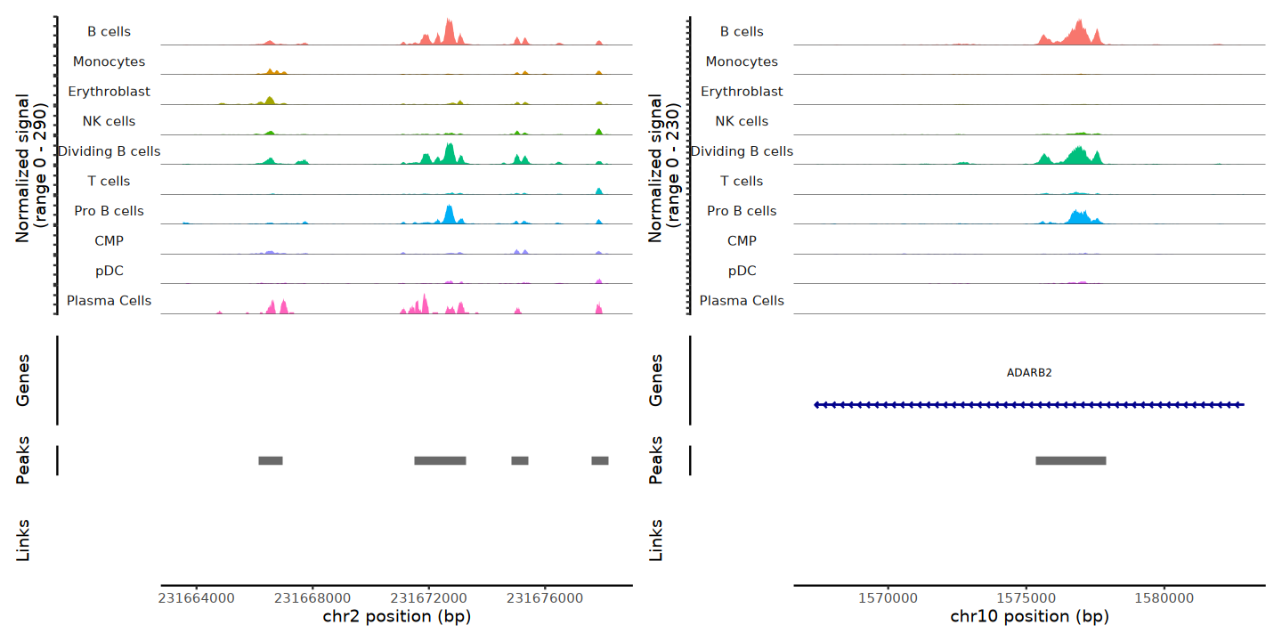
top.da.peak <- rownames(da_peaks[da_peaks$p_val < 0.005 & da_peaks$pct.1 > 0.2, ])

head(top.da.peak)

1. 'chr2-231671510-231673282'
2. 'chr10-1575356-1577892'
3. 'chr15-90190821-90192528'
4. 'chr12-113074961-113076104'
5. 'chr7-74100205-74102036'
6. 'chr2-136206351-136207902'

DefaultAssay(seu) <- "ATAC"
P1 = CoveragePlot(
    object = seu,
    region = top.da.peak[1],
    extend.upstream = 8000,
    extend.downstream = 5000
)
P2 = CoveragePlot(
    object = seu,
    region = top.da.peak[2],
    extend.upstream = 8000,
    extend.downstream = 5000
)

options(repr.plot.width=12, repr.plot.height=6)
patchwork::wrap_plots(P1, P2, ncol = 2)

output

Warning message:
"Removed 28 rows containing missing values or values outside the scale range
(\`geom_segment()\`)."

Warning message:
"Removed 1 row containing missing values or values outside the scale range
(\`geom_segment()\`)."

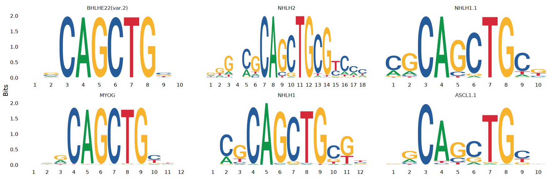
9.2 Motif Enrichment Analysis of Differential Peaks

For the set of differentially accessible peaks selected, test whether any DNA motifs are over-represented. Using a hypergeometric test, evaluate whether the motif is significantly enriched in the differential peaks relative to a GC-content-matched background peak set.

# Get a list of motif position frequency matrices from the JASPAR database
pfm <- getMatrixSet(
  x = JASPAR2020,
  opts = list(collection = "CORE", tax_group = 'vertebrates', all_versions = TRUE)
)

# add motif information
seu <- AddMotifs(
  object = seu,
  genome = BSgenome.Hsapiens.UCSC.hg38,
  pfm = pfm
)

head(rownames(da_peaks))

1. 'chr2-231671510-231673282'
2. 'chr10-1575356-1577892'
3. 'chr15-90190821-90192528'
4. 'chr12-113074961-113076104'
5. 'chr7-74100205-74102036'
6. 'chr2-136206351-136207902'

peak_names <- rownames(da_peaks)
peak_metadata <- seu@assays$ATAC@meta.features[peak_names, ]

has_na <- apply(peak_metadata, 1, function(x) any(is.na(x)))

valid_peaks <- peak_names[!has_na]

if(length(valid_peaks) > 0) {
  enriched.motifs <- FindMotifs(
    object = seu,
    features = valid_peaks
  )
} else {
  message("no motif")
}

options(repr.plot.width = 15, repr.plot.height = 5)
MotifPlot(
  object = seu,
  motifs = head(rownames(enriched.motifs))
)

output

Warning message:
"The \`\` argument of \`guides()\` cannot be \`FALSE\`. Use "

none" instead as
of ggplot2 3.3.4.
ℹ The deprecated feature was likely used in the ggseqlogo package.
Please report the issue at ."

9.3 Differential Peak Annotation

By annotating differentially accessible peaks to their neighboring genes, establish associations between chromatin accessibility and gene expression. This analysis helps interpret the role of differentially accessible peaks in transcriptional regulation, identify their potential target genes, and provides a basis for subsequent biological function analysis.

closest_genes <- ClosestFeature(seu, rownames(da_peaks))

head(closest_genes)

A data.frame: 6 × 8

	tx_id	gene_name	gene_id	gene_biotype	type	closest_region	query_region	distance
	<chr>	<chr>	<chr>	<chr>	<fct>	<chr>	<chr>	<int>
ENSE00001940067	ENST00000466801	PTMA	ENSG00000187514	protein_coding	exon	chr2-231706895-231707228	chr2-231671510-231673282	33612
ENST00000381312	ENST00000381312	ADARB2	ENSG00000185736	protein_coding	gap	chr10-1379161-1737050	chr10-1575356-1577892	0
ENST00000559792	ENST00000559792	SEMA4B	ENSG00000185033	protein_coding	utr	chr15-90191928-90192026	chr15-90190821-90192528	0
ENST00000257600	ENST00000257600	DTX1	ENSG00000135144	protein_coding	gap	chr12-113058452-113077423	chr12-113074961-113076104	0
ENST00000538333	ENST00000538333	LIMK1	ENSG00000106683	protein_coding	gap	chr7-74099239-74105874	chr7-74100205-74102036	0
ENSE00001587001	ENST00000241393	CXCR4	ENSG00000121966	protein_coding	exon	chr2-136118046-136118165	chr2-136206351-136207902	88185

9.4 Peak–Gene Linkage Analysis

By computing the correlation between gene expression and the accessibility of nearby chromatin regions (Peaks), identify potential cis-regulatory elements. The analysis corrects for potential confounders including GC content, overall accessibility background, and peak size.

DefaultAssay(seu) <- "ATAC"

# first compute the GC content for each peak
seu <- RegionStats(seu, genome = BSgenome.Hsapiens.UCSC.hg38)

# link peaks to genes
seu <- LinkPeaks(
  object = seu,
  peak.assay = "ATAC",
  expression.assay = "RNA",
  genes.use = c("MS4A1", "BACH2", "PAX5")
)

p3 <- CoveragePlot(
  object = seu,
  region = "MS4A1",
  features = "MS4A1",
  expression.assay = "RNA",
  extend.upstream = 2000,
  extend.downstream = 2000
)

p4 <- CoveragePlot(
  object = seu,
  region = "BACH2",
  features = "BACH2",
  expression.assay = "RNA",
  extend.upstream = 2000,
  extend.downstream = 2000
)

patchwork::wrap_plots(p3, p4, ncol = 2)

output

Warning message:
"Removed 26 rows containing missing values or values outside the scale range
(\`geom_segment()\`)."

9.5 Footprint Analysis

Motif enrichment analysis of differential peaks can suggest candidate regulatory transcription factors, while footprint analysis goes one step further: by detecting the DNase cleavage protection signal produced when transcription factors bind, it directly identifies the active transcription factor binding sites that are actually exerting regulatory functions in the cell — upgrading the evidence level from "potential binding" to "actively functioning."

# gather the footprinting information for sets of motifs
seu <- Footprint(
  object = seu,
  motif.name = "CEBPA"),
  genome = BSgenome.Hsapiens.UCSC.hg38
)

# plot the footprint data for each group of cells
p2 <- PlotFootprint(seu, features = "CEBPA")

options(repr.plot.width = 12, repr.plot.height = 7)
p2 + patchwork::plot_layout(ncol = 1)

output

Warning message:
"Removed 5090 rows containing missing values or values outside the scale range
(\`geom_label_repel()\`)."

10. Saving Results

saveRDS(seu, file = "processed.rds")