ATAC + RNA Multi-omics: Transcription Factor Footprint Analysis

Author: SeekGene

Time: 12 min

Words: 2.2k words

Updated: 2026-07-07

Reads: 0 times

1. Tutorial Introduction

This tutorial is based on Seurat and Signac and other single-cell multi-omics analysis tools, specifically designed for transcription factor Footprint analysis on SeekArc single-cell multi-omics data (scRNA-seq + scATAC-seq).

In single-cell ATAC-seq analysis, while motif enrichment analysis can tell us which transcription factor binding sites are enriched in specific cell populations or differentially accessible regions, it cannot prove whether transcription factors are actually bound there.

Transcription factor Footprint analysis objectively evaluates the potential physical binding behavior of TFs at the chromatin cleavage trajectory level. Its basic principle is: when a TF binds to DNA, it blocks Tn5 enzyme from cleaving that region, thereby forming a relatively low-signal protected zone (i.e., "footprint") at the center of the enrichment peak, with signal peaks on both sides.

By comparing the changes in the depth of this protected zone across different cell populations or experimental groups, it is possible to further verify whether candidate transcription factors have undergone real binding and unbinding events in the target state.

suppressPackageStartupMessages(suppressWarnings({
    library(presto)
    library(Seurat)
    library(BiocGenerics)
    library(S4Vectors)
    library(IRanges)
    library(Signac)
    library(ComplexHeatmap)
    library(Biobase)
    library(AnnotationDbi)
    library(org.Hs.eg.db)
    #library(org.Mm.eg.db)
    library(GenomicRanges)
    library(JASPAR2020)
    library(TFBSTools)
    library(memuse)
    library(stringr)
    library(dplyr)
    library(foreach)
    library(doParallel)
    library(base64enc) 
}))

2. Input File Preparation

2.1 Input File Requirements

Before starting the analysis, the following core input files need to be prepared:

• input.rds: Preprocessed Seurat object file. This object must contain both RNA and ATAC assays.
• meta.tsv: Cell metadata file (tab-delimited). Must include a barcode column, as well as corresponding columns for defining cell types (e.g., Celltype) and sample groups (e.g., Sample).
• genome.fa: Reference genome FASTA file for the corresponding species. Used for extracting DNA sequences.
• ATAC fragment file and index: The fragments.tsv.gz and its .tbi index file that the ATAC assay depends on. This is the most core file for Footprint analysis.

# --- Input Parameter Configuration --- Fill in parameters here according to your own needs

## fpath: Directory where fragment files are located
fpath = "/path/to/PBMC_demo"

## rds: Path to the input Seurat object RDS file, containing pre-processed single-cell multi-omics data
rds = "/path/to/input.rds"

## meta: Metadata file path (TSV format), containing sample information, cell-type annotations, and other metadata
meta = "/path/to/meta.tsv"

## species: Species information
species="human"

## ref_genome: Path to the reference genome FASTA file, used for genomic sequence alignment and annotation
ref_genome = "/path/to/genome.fa"

## clusters_col: Column name in the metadata used to identify cell type / clustering
clusters_col = "Celltype"

## celltypes: List of cell types to be analyzed; multiple cell types separated by commas
celltypes = "B cells,CMP,Dividing B cells,Erythroblast,NK cells,pDC,Plasma Cells,Pro B cells,T cells"

## downsample: Whether to perform cell downsampling; TRUE enables downsampling to balance cell counts across cell types
downsample = "TRUE"

## downsample_num: Target cell count after downsampling; maximum number of cells retained per cell type
downsample_num = "3000"

## motif_names: List of Motif names for Footprint analysis; multiple names separated by commas.
tf_names = "GATA2,CEBPA,EBF1"

output <- "."
footprint_dir <- paste0(output, "/footprint")
dir.create(footprint_dir, recursive = TRUE, showWarnings = FALSE)
celltypes <- strsplit(celltypes,",")[[1]]
downsample_num <- as.numeric(downsample_num)
tf_list <- strsplit(tf_names, ",")[[1]]

3. Data Loading and Preprocessing

3.1 Loading Seurat Object and Metadata

obj <- readRDS(rds)
if (meta != ""){
  meta <- read.table(meta,header=T,sep='	',check.names=F)
  rownames(meta) <- meta$barcode
  obj <- AddMetaData(obj, meta)
}
obj <- subset(obj, subset = !!sym(clusters_col) %in% celltypes)

3.2 Cell Type Filtering and Downsampling Balance

if (downsample == "TRUE"){
  cells_to_keep <- c()
  for (ctype in celltypes) {
    ctype_cells <- rownames(obj@meta.data[obj@meta.data[[clusters_col]] == ctype, ])
    if (length(ctype_cells) > downsample_num) {
      ctype_cells <- sample(ctype_cells, downsample_num)
    }
    cells_to_keep <- c(cells_to_keep, ctype_cells)
  }
  obj <- subset(obj, cells = cells_to_keep)
}

3.3 Modifying Fragment File Paths

In the ATAC modality of the Seurat object, fragment files do not store massive sequences directly in memory, but only save the file paths on disk (Paths). Therefore, when data is transferred between different servers or containers, the old paths originally saved in the object often become invalid due to changes in directory structure or permission issues, making subsequent reads impossible. The code here iterates through all fragment records in the object, extracts the file names, and re-concatenates them with our specified latest valid directory (fpath) to achieve real-time path updates.

n_fragments <- length(obj@assays$ATAC@fragments)
for (i in 1:n_fragments) {
  original_path <- obj@assays$ATAC@fragments[[i]]@path
  filename <- basename(original_path)
  obj@assays$ATAC@fragments[[i]]@path <- paste0(fpath, '/', filename)
}

3.4 Preparing the Reference Genome

A core challenge in Footprint analysis is Tn5 sequence bias correction. The Tn5 enzyme is not completely random when cleaving DNA; it has an inherent cleavage preference for specific hexamer sequences. If this preference error caused by the DNA sequence itself is not removed, the signal trough ("footprint") we observe may simply be because the sequence in that region happens to be difficult for Tn5 to cleave, rather than a transcription factor actually binding and protecting it.

To accurately calculate and correct this sequence preference, the underlying algorithm must obtain the true DNA base sequence of each peak region, so we need to load and align the reference genome.

DefaultAssay(obj) <- "ATAC"
Idents(obj) <- clusters_col

library(Biostrings)
genome <- readDNAStringSet(ref_genome)
names(genome) <- sub(" .*", "", names(genome)) 
keep_chromosomes <- unique(as.character(seqnames(granges(obj[["ATAC"]]))))
genome <- genome[which(names(genome) %in% keep_chromosomes)]
obj@assays$ATAC@ranges <- keepSeqlevels(granges(obj),keep_chromosomes, pruning.mode="coarse")

genome_seqlens <- setNames(as.numeric(width(genome)), names(genome))

if (species == "human"){
    pfm <- getMatrixSet(x = JASPAR2020, opts = list(species = 9606, all_versions = TRUE))
} else if (species == "mouse"){
    pfm <- getMatrixSet(x = JASPAR2020, opts = list(species = 10090, all_versions = TRUE))
} else {
    stop(paste0("The value of 'species' is not supported."))
}

#将 Motif 信息添加至 ATAC Assay
obj <- AddMotifs(object = obj, genome = genome, pfm = pfm)

💡 Code Processing Details:

The Signac official tutorial requires installing species-specific BSgenome R packages. To avoid the risk of installation failures or version inconsistencies, this tutorial uses Biostrings::readDNAStringSet() to directly read custom FASTA files instead.

Emphasis: The ref_genome (FASTA file) passed here must be exactly the same as the reference genome FASTA file used during the upstream sequence alignment (e.g., when using SeekArcTools), otherwise it will cause coordinate misalignment and completely wrong Footprint results.

In addition, the code performs strict chromosome name cleaning (removing redundant descriptors from FASTA headers) and implements forced alignment with the chromosomes internal to the ATAC object. This processing actively removes stray chromosomes (Scaffolds/Contigs) that do not appear in the ATAC matrix, significantly reducing memory consumption and completely eliminating out-of-bound errors caused by chromosome mismatches.

4. Footprint Analysis and Visualization

Since calculating Footprint involves a large amount of underlying sequence traversal and is time-consuming, it is recommended to enable parallel computing.

if (requireNamespace("future", quietly = TRUE)) {
    cores <- parallelly::availableCores()
    workers <- as.integer(floor(cores * 0.7))
    
    if (.Platform$OS.type == "unix") {
        future::plan(future::multicore, workers = workers)
    } else {
        future::plan(future::multisession, workers = workers)
    }

}

if (requireNamespace("memuse", quietly = TRUE)) {
    total_mem <- as.numeric(memuse::Sys.meminfo()$totalram)
    options(future.globals.maxSize = total_mem * 0.7)
} else {
    options(future.globals.maxSize = 50 * 1024^3)
}

output

Footprint 并行计算已启动，总核心数=32，使用 22 个工作线程

4.1 Extracting the Footprint Matrix

We use the Footprint() function to extract the Tn5 insertion signal matrix near a specific motif. This process locates peak regions containing the motif and finely statistics the distribution frequency of cleavage events within a certain range upstream and downstream (default ±250 bp).

Biological questions it can answer By statistics Tn5 cleavage trajectories, we can directly and objectively observe: whether a transcription factor has undergone real physical binding at its motif binding site, and successfully blocked Tn5 enzyme cleavage to form a low-signal "footprint protected zone".

motif_obj <- Motifs(obj[["ATAC"]])
motif_names_all <- as.character(motif_obj@motif.names)
motif_ids_all <- names(motif_obj@motif.names)

motifs_use <- c()
for (tf in tf_list) {
    idx <- grep(paste0("^", tf, "$"), motif_names_all, ignore.case = TRUE)
    if (length(idx) == 0) {
        idx <- grep(tf, motif_names_all, ignore.case = TRUE)
    }
    if (length(idx) > 0) {
        motifs_use <- c(motifs_use, motif_names_all[idx[1]])
        message(paste0("Found Motif name for ", tf, ": ", motif_names_all[idx[1]]))
    } else {
        warning(paste0("Warning: Motif for TF ", tf, " not found in the Seurat object."))
    }
}
motifs_use <- unique(motifs_use)
if (length(motifs_use) == 0) {
    stop("Error: None of the provided TF names were found in the Motif database.")
}

atac_ranges <- granges(obj[["ATAC"]])
valid_chr <- intersect(as.character(seqlevels(atac_ranges)), names(genome_seqlens))
atac_ranges <- keepSeqlevels(atac_ranges, valid_chr, pruning.mode = "coarse")
seqlengths(atac_ranges)[valid_chr] <- genome_seqlens[valid_chr]     

atac_ranges <- trim(atac_ranges)
keep_idx <- start(atac_ranges) >= 1 & end(atac_ranges) <= seqlengths(atac_ranges)[as.character(seqnames(atac_ranges))]
keep_idx[is.na(keep_idx)] <- FALSE
obj[["ATAC"]]@ranges <- atac_ranges[keep_idx]
DefaultAssay(obj) <- "ATAC"

fp_obj <- NULL
use_fallback <- FALSE
tryCatch({
    fp_obj <- Footprint(
        object = obj,
        motif.name = motifs_use,
        genome = genome,
        assay = "ATAC"
    )
}, error = function(e1) {
    message("Direct footprint calculation failed, attempting to filter using safe boundaries... Error reason:", e1$message)
    up <- 250
    down <- 250
    motif_obj <- Motifs(obj[["ATAC"]])
    region_list <- list()
    key_vec <- c()
    for (m in motifs_use) {
        regs <- Signac:::GetFootprintRegions(motif.obj = motif_obj, motif.name = m)
        regs <- keepSeqlevels(regs, intersect(seqlevels(regs), names(genome_seqlens)), pruning.mode = "coarse")
        chr_len <- genome_seqlens[match(as.character(seqnames(regs)), names(genome_seqlens))]
        ok <- !is.na(chr_len) & start(regs) > up & end(regs) <= (chr_len - down)
        regs <- regs[ok]
        if (length(regs) > 0) {
            region_list[[length(region_list) + 1]] <- regs
            key_vec <- c(key_vec, m)
        }
    }
    if (length(region_list) == 0) {
        stop("Fallback failed: No valid motif regions remain after boundary filtering.")
    }
    fp_obj <<- Footprint(
        object = obj,
        regions = region_list,
        key = key_vec,
        genome = genome,
        assay = "ATAC",
        upstream = up,
        downstream = down,
        compute.expected = FALSE
    )
    motifs_use <<- key_vec
    use_fallback <<- TRUE
})

if (is.null(fp_obj)) {
    stop("Final footprint calculation failed.")
}

💡 Advanced Notes: Why is the code in this tutorial much more complex than the official single-line Footprint() call?

Ideally, running Footprint(obj, motif.name = "GATA2") directly would be sufficient. However, in real single-cell analysis scenarios, simple calls are highly prone to errors and crashes due to underlying data formats or edge details. To ensure extremely high robustness of the analysis workflow, we have built in the following automatic fault-tolerance mechanisms in the script:

1. Smart TF Name Matching: Users usually prefer to enter readable TF short names (e.g., "GATA2"), while the underlying database often has specific complex naming (e.g., "GATA2::CEBPA", etc.). The code has built-in case-insensitive and fuzzy matching logic to automatically bridge readable names with underlying motif IDs.
2. Strict Chromosome Information Alignment: ATAC peak data often contains unassembled scattered chromosome fragments (Scaffolds/Contigs). If the reference genome does not contain these fragments, extracting sequences will cause fatal errors. The code automatically intercepts and cleans these unmatched fragments.
3. Safe Cropping of Out-of-bounds Peaks: Footprint calculation requires extracting DNA sequences upstream and downstream of the motif center position. If a peak is located near the end of a chromosome, the required extension range may exceed the chromosome boundary, triggering out-of-bounds errors. The code automatically checks each peak: if the required extension exceeds the chromosome length, it is safely cropped to the maximum available range, ensuring that no single peak causes the entire program to crash.

4.2 Visualizing Footprint Results

After obtaining the Footprint matrix, we can use the PlotFootprint() function for visualization. We can compare different cell types, or compare footprint depth differences between different groups within the same cell type.

if (use_fallback) {
    p_fp_cluster <- PlotFootprint(
        object = fp_obj,
        features = motifs_use,
        group.by = clusters_col,
        assay = "ATAC",
        show.expected = FALSE,
        normalization = "subtract"
    )
} else {
    p_fp_cluster <- PlotFootprint(
        object = fp_obj,
        features = motifs_use,
        group.by = clusters_col,
        assay = "ATAC"
    )
}

options(repr.plot.width = 10, repr.plot.height = 10)

p_fp_cluster + patchwork::plot_layout(ncol = 1)

output

Warning message:
“Removed 4545 rows containing missing values or values outside the scale range
(\`geom_label_repel()\`).”
Warning message:
“Removed 4599 rows containing missing values or values outside the scale range
(\`geom_label_repel()\`).”
Warning message:
“Removed 4599 rows containing missing values or values outside the scale range
(\`geom_label_repel()\`).”

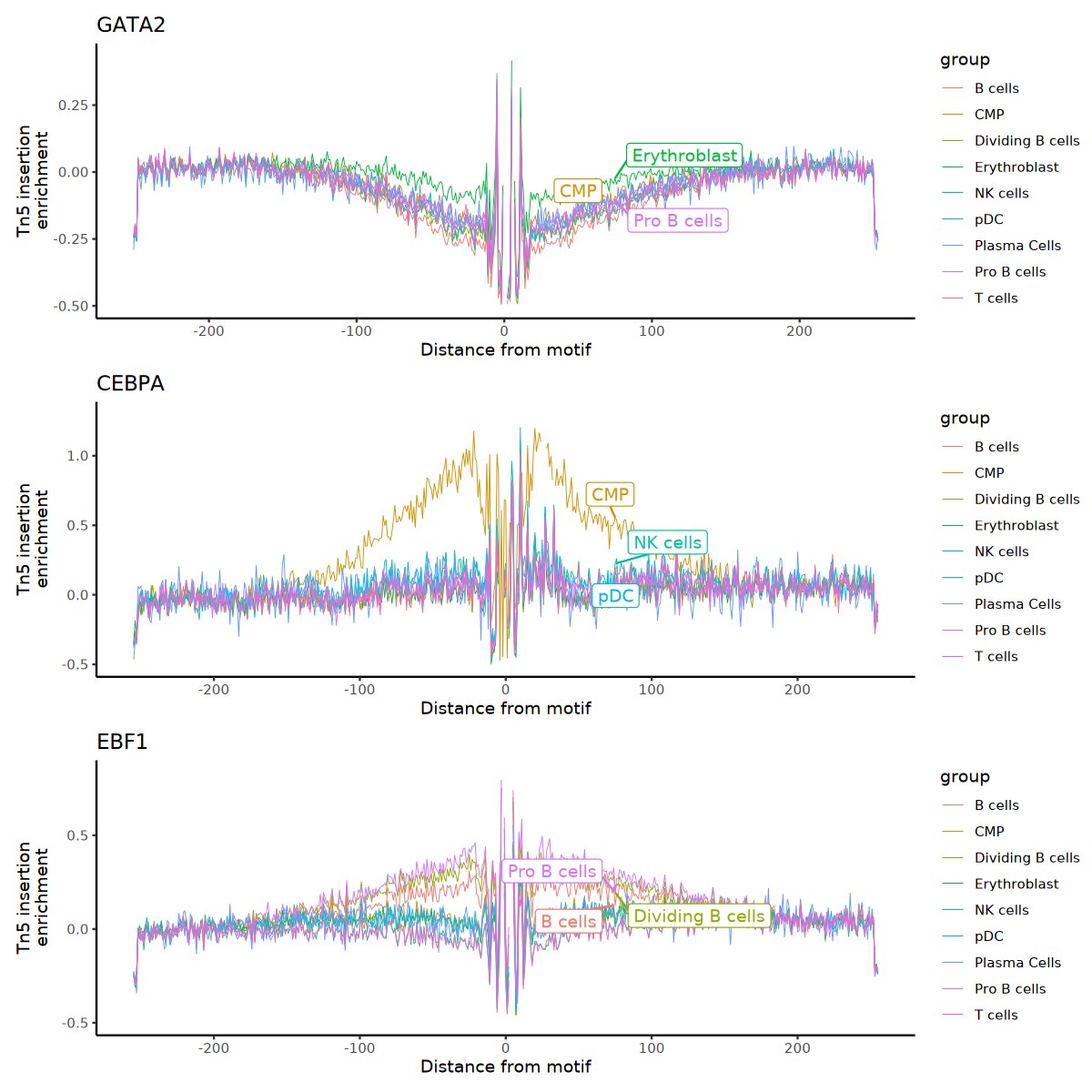
Notes:

1. X-axis represents the distance from the motif center (bp).
2. Y-axis represents the normalized Tn5 cleavage frequency.
3. If you see a clear "depression" at the center (0 bp) (i.e., reduced cleavage frequency), with "peaks" on both sides, this indicates that the transcription factor has undergone real binding in these cells.
4. If the depression in one group (e.g., Case group) is deeper than another group (e.g., Control group), it indicates that the transcription factor has stronger binding activity in the Case group.