ataCNV Analysis Tutorial: Tumor Copy Number Variation Resolution Based on scATAC-seq
Background
Chromosomal Copy Number Variation (CNV) is a hallmark of tumor genomic instability, characterized by large-scale amplification or deletion of chromosomal segments. CNV drives tumorigenesis, progression, and therapeutic resistance by altering the copy number of oncogenes (e.g., MYC) or tumor suppressor genes (e.g., TP53) and inducing gene dosage effects. Resolving CNV at single-cell resolution is crucial for revealing tumor heterogeneity: relying on malignant cell-specific CNV profiles (e.g., chromosome 7 amplification, chromosome 10 deletion), tumor cells can be distinguished from non-malignant cells (e.g., T cells, fibroblasts) in complex microenvironments, further elucidating subclonal structures and epigenetic regulatory differences.
Compared to CNV inference based on scRNA-seq, scATAC-seq uses genomic coverage as a direct signal, unaffected by transcriptional programs and transient expression fluctuations; it also has more uniform coverage in non-transcribed regions, thus offering higher resolution and robustness for large-segment and fine-grained CNV. ataCNV is one of the tools specifically designed for inferring CNV from scATAC-seq data, using coverage counts in fixed genomic windows as proxy signals for DNA copy status to identify chromosomal segment amplification/deletion events at the single-cell level, thereby achieving malignant vs. non-malignant cell differentiation and fine subclonal characterization.
Purpose and Significance
- Cell-level Tumor Identification: Precisely distinguish malignant cells from microenvironmental cells based on CNV profiles
- Subclonal Heterogeneity Resolution: Reconstruct copy number evolutionary trajectories to understand clonal competition and differentiation relationships
- Multi-omics Integrated Interpretation: Integrate CNV with chromatin accessibility and cell annotation/clustering results to elucidate the impact of genomic structural changes on epigenetic regulation and cell states
- Clinical Translational Value: Provide structural variation evidence for prognostic stratification, efficacy assessment, and potential target mining
ataCNV Algorithm Principles
ataCNV mainly includes two core steps:
Normalization Step:
- Generate single-cell read count matrices on 1 million base pair (Mbp) genomic intervals
- Filter cells and genomic intervals based on mappability and number of zero entries
- Smooth the count matrix using a first-order dynamic linear model to reduce extreme noise
- Perform cell-wise local regression to eliminate potential biases caused by GC content
- Normalize using normal cell data to deconvolve copy number signals from other confounding factors like chromatin accessibility
Segmentation Step:
- Apply multi-sample BIC-seq algorithm for joint segmentation of all single cells
- Estimate the copy ratio of obtained segments in each cell
- Calculate the burden score for each cell group and classify groups with high CNA burden as malignant cells
Parameter Settings
Please first mount the cloud platform process data to be analyzed. For mounting methods, please refer to the jupyter usage tutorial.
Specific parameter entry:
- rds: The process-related rds file mounted, which is the process-related Seurat object;
- meta: The process-related meta file mounted, which is the meta.data inside the process-related Seurat object;
- outdir: Output directory path for storing analysis results;
- species: Species information, only supports human;
- SAMplenames: Sample names, supports multiple samples, separated by commas;
- mode: Analysis mode, supports three modes:
normalcells: Use specified normal cell types for normalizationallcells: Identify normal cells after clustering using all cellsnone: Do not perform normalization
- celltype_col: Cell type column name, select the label corresponding to the cell type to be analyzed;
- cluster_col: Cell cluster column name, used for cell grouping information;
- Normal_celltype: Normal cell type name, used when mode is "normalcells"
# Parameters
#rds = "/PROJ2/STANDARD/scATAC/Signac/example_data/25020230_CC_T/result.rds"
#meta = "/PROJ2/STANDARD/scATAC/Signac/example_data/25020230_CC_T/meta.tsv"
#outdir = "/PROJ2/FLOAT/advanced-analysis/Seek_module_dev/ataCNV/demo/output/"
#species = "human"
#samplenames = "CC_T_A"
#celltype_col = "CellAnnotation"
#cluster_col = ""
#Normal_celltype = "T_cells"
#mode = "normalcells"# Parameters
rds = "/PROJ2/FLOAT/advanced-analysis/test/2388-5504-6420-584654738725821050/input.rds"
meta = "/PROJ2/FLOAT/advanced-analysis/test/2388-5504-6420-584654738725821050/meta.txt"
outdir = "/PROJ2/FLOAT/advanced-analysis/test/2388-5504-6420-584654738725821050/output/"
species = "human"
samplenames = "joint14_A"
mode = "normalcells"
celltype_col = "CellAnnotation"
cluster_col = "wknn_res.0.5_d30_l2_50"
Normal_celltype = "T_cells"Environment Preparation
R Package Loading
Please select the common_r environment for this integrated tutorial.
Data Preprocessing
Load and process single-cell ATAC-seq data to prepare for CNV analysis. Main steps include:
- Data Loading: Read Seurat object and metadata file
- Cell Filtering: Filter low-quality cells based on QC standards
- Genome Setting: Set the corresponding genome version based on species information
- Count Matrix Extraction: Extract gene activity count matrix from Seurat object
options(warn = -1)
suppressWarnings({
  suppressMessages({
      library(data.table)
      library("AtaCNV")
      library(Matrix)
      library(Seurat,lib.loc="/PROJ2/FLOAT/shumeng/apps/miniconda3/envs/Geneactivity/lib/R/library")
      library(Signac,lib.loc="/PROJ2/FLOAT/shumeng/apps/miniconda3/envs/Geneactivity/lib/R/library")
      library(dplyr)
      library(png)
      library(ComplexHeatmap)
      library(RColorBrewer)
           })
})
options(warn = 0)
Start CNV Analysis
Start executing the ataCNV CNV inference pipeline. This pipeline converts scATAC-seq fragment data into coverage matrices of fixed genomic windows, resolving chromosomal copy number variations at the single-cell level through noise control and event identification.
Execution Steps Overview:
- Data Normalization: Normalize the count matrix based on the selected mode
- CNV Inference: Call BIC-seq algorithm for segmentation analysis to identify copy number variation events
- Result Output: Generate matrix tables containing CNV status of each window, supporting subsequent visualization and cell grouping integration
Key Parameter Description:
- Window Size: Default 1Mbp, balancing CNV resolution and statistical robustness
- Normalization Mode: Select different normalization strategies based on the presence of normal cells
- Segmentation Algorithm: Use BIC-seq algorithm for joint segmentation analysis
- Chromosome Handling: Automatically handle all autosomes and sex chromosomes
# Create output directory
dir.create("../result", recursive = TRUE, showWarnings = FALSE)

# Data loading and preprocessing
suppressWarnings({
  suppressMessages({
      samplenames <- unlist(strsplit(samplenames, split = ","))
      meta=read.table(meta, sep = "\t", header = T)
      rownames(meta)=meta$barcodes
  })
})# Load count matrix data
suppressWarnings({
suppressMessages({
if(length(samplenames) >1){
count=list()
for(i in samplenames){
count[[i]] <- readRDS(paste0(outdir, i, "_count.rds"))
count[[i]] <- as.data.frame(count[[i]])
count[[i]]$barcode=rownames(count[[i]])
count=data.table::rbindlist(count)
count <- as.data.frame(count)
rownames(count)=count$barcode
count$barcode=NULL
}
}else{
count <- readRDS(paste0(outdir, samplenames, "_count.rds"))
count <- as.data.frame(count)
}
meta=meta[rownames(meta) %in% rownames(count),]
})
})# Set genome version
if (species == "human") {
genome <- "hg38"
}else {
stop(paste0("Error: Unsupported species '", species, "'. Supported values: human"))
}# Data normalization
options(warn = -1)
suppressWarnings({
suppressMessages({
if(mode=="normalcells"){
norm_re <- AtaCNV::normalize(count,
genome=genome, mode="normal cells",
normal_cells=(meta[[celltype_col]]==Normal_celltype),
output_dir=paste0(outdir,"dir"),
output_name="norm_re.rds"
)
}else if(mode=="allcells"){
norm_re <- AtaCNV::normalize(count,
genome=genome, mode="all cells",
cell_cluster=meta[[cluster_col]],
output_dir=paste0(outdir,"dir"),
output_name="norm_re.rds"
)
}else if(mode=="none"){
norm_re <- AtaCNV::normalize(count,
genome=genome, mode=mode,
cell_cluster=meta[[cluster_col]],
output_dir=paste0(outdir,"dir"),
output_name="norm_re.rds"
)
}
})
})
options(warn = 0)[1] " number of bin before filter: 3102"
[1] " number of bin after filter: 2673"
[1] " number of cells before filter: 16653"
[1] " number of cells after filter: 16653"
[1] "Step 2: smoothing read count signals..."
[1] "Step 3: calculating baseline of normal cells..."
[1] " Baseline is calculated using median read count of normal cells"
[1] "Step 4: normalizing against baseline..."
[1] "99th percentile: 1.83815598812295"
[1] "Step 5: GC correction..."
[1] "Step 6: saving results..."
calculate_CNV <- function (norm_count, baseline, BICseq = "default", lambda = 5,
    min_interval = 2, smooth = F, downsample = 0, output_dir = "./",
    output_name = "CNV_result.rds")
{
    if (BICseq == "default") {
        if (Sys.info()["sysname"] == "Windows") {
            BICseq <- system.file("BICseq2", "mbic-seq.exe",
                package = "AtaCNV")
        }
        else if (Sys.info()["sysname"] == "Linux") {
            BICseq <- system.file("BICseq2", "MBICseq", package = "AtaCNV")
            Sys.chmod(BICseq, mode = "0755")
        }
    }
    if (!dir.exists(output_dir)) {
        dir.create(output_dir)
    }
    if (is.vector(baseline)) {
        baseline <- matrix(data = baseline, nrow = nrow(norm_count),
            ncol = ncol(norm_count), byrow = T)
    }
    bins <- str2bin(colnames(norm_count))
    chr_bkp <- bin2chrbkp(bins)
    print("Running BICseq2 for segmentation...")
    bkp <- c()
    lambda <- lambda
    tmp_dir <- output_dir
    k <- 0
    if (downsample > 0) {
        idx <- sample(1:nrow(norm_count), downsample)
        norm_count_origin <- norm_count
        norm_count <- norm_count[idx, ]
        baseline_origin <- baseline
        baseline <- baseline[idx, ]
    }
    for (i in unique(bins$chr)) {
        print(i)
        if (sum(bins$chr == i) <= 2) {
            next
        }
        norm_count_ <- norm_count[, bins$chr == i]
        bic_input <- matrix(ncol = 2 * nrow(norm_count_) + 2,
            nrow = ncol(norm_count_))
        bic_input[, 1:2] <- as.matrix(str2bin(colnames(norm_count_))[,
            2:3])
        bic_input[, 2 * c(1:nrow(norm_count_)) + 1] <- t(norm_count_)
        bic_input[, 2 * c(1:nrow(norm_count_)) + 2] <- t(baseline[,
            bins$chr == i])
        s <- c(1:ncol(bic_input))
        s[1:2] <- c("start", "end")
        s[2 * c(1:nrow(norm_count_)) + 1] <- rownames(norm_count_)
        s[2 * c(1:nrow(norm_count_)) + 2] <- paste0(rownames(norm_count_),
            "_ref")
        colnames(bic_input) <- s
        write.table(x = bic_input, file = paste0(tmp_dir, i,
            ".bin"), quote = F, sep = "\t", row.names = F, col.names = T,
            append = F)
        system(paste0(BICseq, " -i ", paste0(tmp_dir, i, ".bin"),
            " -l ", lambda))
        if(file.exists(paste0(tmp_dir, i, ".bin_seg"))){
            seg_re <- read.table(paste0(tmp_dir, i, ".bin_seg"),
            header = T, sep = "\t")
            bkp_ <- cumsum(seg_re$binNum)
            bkp <- merge_bkp(bkp, bkp_ + k, min_interval = 2)
        }else{
            warning(paste("Skipping chromosome", i, "because .bin_seg file is missing"))
            k <- k + sum(bins$chr == i)
        }

    }
    for (i in unique(bins$chr)) {
        file.remove(paste0(tmp_dir, i, ".bin"))
        file.remove(paste0(tmp_dir, i, ".bin_seg"))
    }
    bkp <- merge_bkp(chr_bkp, bkp, min_interval = 2)
    bkp <- sort(bkp)
    print(paste0("number of breakpoints: ", length(bkp)))
    if (downsample > 0) {
        norm_count <- norm_count_origin
        baseline <- baseline_origin
    }
    CNV_re <- matrix(0, nrow = nrow(norm_count), ncol = length(bkp) -
        1)
    for (i in 1:(length(bkp) - 1)) {
        if (bkp[i] + 1 == bkp[i + 1]) {
            CNV_re[, i] <- norm_count[, bkp[i + 1]]/baseline[,
                bkp[i + 1]]
            next
        }
        temp <- apply(norm_count[, (bkp[i] + 1):bkp[i + 1]],
            1, mean)/apply(baseline[, (bkp[i] + 1):bkp[i + 1]],
            1, mean)
        CNV_re[, i] <- temp
    }
    CNV <- norm_count
    for (i in 1:(length(bkp) - 1)) {
        CNV[, (bkp[i] + 1):bkp[i + 1]] <- matrix(CNV_re[, i],
            nrow = nrow(CNV), ncol = bkp[i + 1] - bkp[i])
    }
    if (smooth) {
        print("smoothing...")
        CNV <- smooth_CNV(CNV)
    }
    print("Saving results...")
    CNV <- round(CNV, digit = 3)
    result <- list(copy_ratio = CNV, bkp = bkp, CNV_seg = CNV_re)
    saveRDS(result, file = paste0(output_dir, output_name))
    return(result)
}# CNV segmentation analysis
suppressWarnings({
suppressMessages({
seg_re <- calculate_CNV(norm_count=norm_re$norm_count,
baseline=norm_re$baseline,
output_dir=paste0(outdir,"dir/"),
output_name="seg_re.rds")
})
})[1] "chr1"
[1] "chr2"
[1] "chr3"
[1] "chr4"
[1] "chr5"
[1] "chr6"
[1] "chr7"
[1] "chr8"
[1] "chr9"
[1] "chr10"
[1] "chr11"
[1] "chr12"
[1] "chr13"
[1] "chr14"
[1] "chr15"
[1] "chr16"
[1] "chr17"
[1] "chr18"
[1] "chr19"
[1] "chr20"
[1] "chr21"
[1] "chr22"
[1] "chrX"
[1] "chrY"
[1] "number of breakpoints: 55"
[1] "Saving results..."
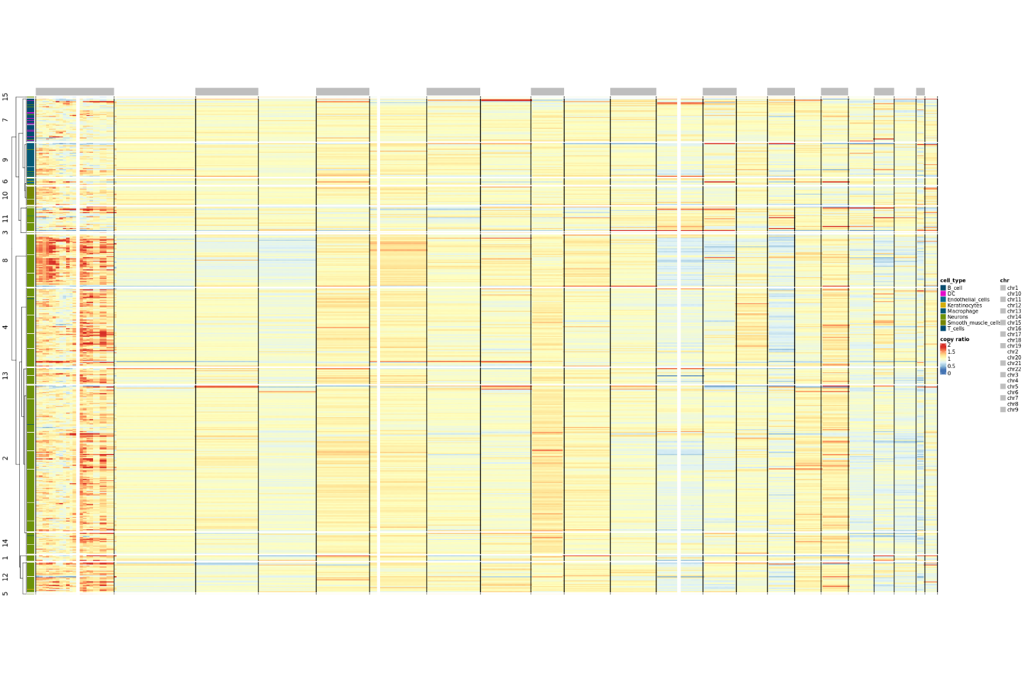
Heatmap Visualization
Visualize cell copy number variations using a heatmap. The color ribbons on the left side of the heatmap indicate cells arranged by cell type and cell clustering. Each row represents a cell, and each column represents a chromosome arm. The heatmap color represents the copy ratio. A copy ratio near 1 indicates normal diploidy; a copy ratio between 0-1 indicates chromatin deletion, with values closer to 0 (bluer color) indicating more severe deletion; a copy ratio between 1-2 indicates chromatin amplification, with values closer to 2 (redder color) indicating more severe amplification.
# Generate CNV heatmap
options(warn = -1)
suppressWarnings({
  suppressMessages({
      plot_heatmap(copy_ratio=seg_re$copy_ratio,
             cell_cluster=meta[[cluster_col]],
             cell_annotation=meta[[celltype_col]],
             output_dir="../result/",
             output_name="copy_ratio.png")
      #plot=readPNG("../result/copy_ratio.png")
      plot <- png::readPNG("../result/copy_ratio.png")
      options(repr.plot.width = 12, repr.plot.height = 8)
      grid::grid.raster(plot)
     })
})
options(warn = 0)[1] "Step 2: plotting..."
Result Files
├── copy_ratio.png Copy Number Variation Heatmap
Result Directory: The directory includes all images and table files involved in this analysis
Appendix
.txt: Result data table files, separated by tabs. Unix/Linux/Mac users use less or more commands to view; Windows users use advanced text editors like Notepad++, or open with Microsoft Excel.
.pdf: Result image files, vector graphics, can be zoomed in/out without distortion, convenient for viewing and editing, can be edited using Adobe Illustrator for publication.
.rds: Seurat object containing gene activity assay, needs to be opened in R environment for viewing and further analysis.