CellCharter Spatial Transcriptomics Analysis: Spatial Domain Identification and Cellular Microenvironment Resolution
Background
The algorithm principle is as follows:
CellCharter first constructs a spatial network based on the spatial coordinates of cells or spots. In this network, each cell or spot is treated as a node, and connections between nodes are based on their spatial proximity.
Neighborhood Enrichment Analysis: CellCharter calculates the number of connections between two cell groups and compares it with random expectations.
Observed: The actual number of connections between two cell groups.
Expected: The random expected number of connections based on node degrees.
Neighborhood Enrichment Score (NE) is the ratio of Observed to Expected: NE = Observed/Expected
Differential Neighborhood Enrichment Analysis
CellCharter can also compare neighborhood enrichment analysis results under different conditions (e.g., health vs. disease) and calculate Differential Neighborhood Enrichment Scores (Differential NE).
The Differential Neighborhood Enrichment Score is the difference between neighborhood enrichment scores under two conditions. To assess the significance of the difference, CellCharter can calculate P-values by randomly sampling condition labels.
CellCharter's neighborhood enrichment analysis reveals spatial interactions of cells in tissues by constructing spatial networks, calculating spatial proximity between cell groups, and comparing with random expectations. Its asymmetric neighborhood enrichment analysis further reveals preferential connections between cell groups, while differential neighborhood enrichment analysis is used to compare changes in spatial interactions under different conditions.
CellCharter Calculation Results
Load Required Packages
import squidpy as sq
import cellcharter as cc
import scanpy as sc
import pandas as pd
import matplotlib.pyplot as plt
from itertools import combinations
import matplotlib.image as mpimg
import oswarnings.warn('nopython is set for njit and is ignored', RuntimeWarning)
/PROJ2/FLOAT/jinwen/apps/miniconda3/envs/cellcharter-env/lib/python3.9/site-packages/tqdm/auto.py:21: TqdmWarning: IProgress not found. Please update jupyter and ipywidgets. See https://ipywidgets.readthedocs.io/en/stable/user_install.html
from .autonotebook import tqdm as notebook_tqdm
meta_path="../../data/AY1748480899609/meta.tsv"
col_sam="Sample"
sample_name="N1_expression,N2_expression"
col_celltype="CellAnnotation"
col_group="Sample"sample_name=sample_name.strip().split(",")Read Data
adata = sc.read_10x_mtx("filtered_feature_bc_matrix/",cache=False)

## Add Coordinate Information
spatial_df = pd.read_csv("filtered_feature_bc_matrix/cell_locations.tsv",index_col=0,sep='\t')
spatial_df1 = spatial_df[spatial_df.index.isin(adata.obs_names)]
adata.obsm["spatial"] = spatial_df1.values
meta_df = pd.read_csv(meta_path,index_col=0,sep='\t')
meta_df = meta_df.reindex(adata.obs_names)
adata.obs = pd.concat([adata.obs, meta_df], axis=1)adata.obs[col_sam] = adata.obs[col_sam].astype('category')
adata.obs[col_celltype] = adata.obs[col_celltype].astype('category')sq.gr.spatial_neighbors(adata, library_key=col_sam, coord_type='generic', delaunay=True)Single Sample Cell Type Colocalization
Evaluate whether the spatial proximity between two cell groups (or cell states) is higher than random expectation.
for i in range(len(sample_name)):
    adata1 = adata[adata.obs[col_sam] == sample_name[i]]
    cc.gr.nhood_enrichment(
        adata1,
        cluster_key=col_celltype,
    )

    cc.pl.nhood_enrichment(
        adata1,
        cluster_key=col_celltype,
        annotate=True,
        vmin=-0.1,
        vmax=0.1,
        figsize=(5,5),
        fontsize=7,
        title=sample_name[i]+" Neighborhood enrichment",
        save="./"+sample_name[i]+"_"+col_celltype+"_enrichment_heatmap.png"
)adata.uns[f"{cluster_key}_nhood_enrichment"] = result
/PROJ2/FLOAT/jinwen/apps/miniconda3/envs/cellcharter-env/lib/python3.9/site-packages/cellcharter/gr/_nhood.py:236: ImplicitModificationWarning: Trying to modify attribute \`._uns\` of view, initializing view as actual.
adata.uns[f"{cluster_key}_nhood_enrichment"] = result
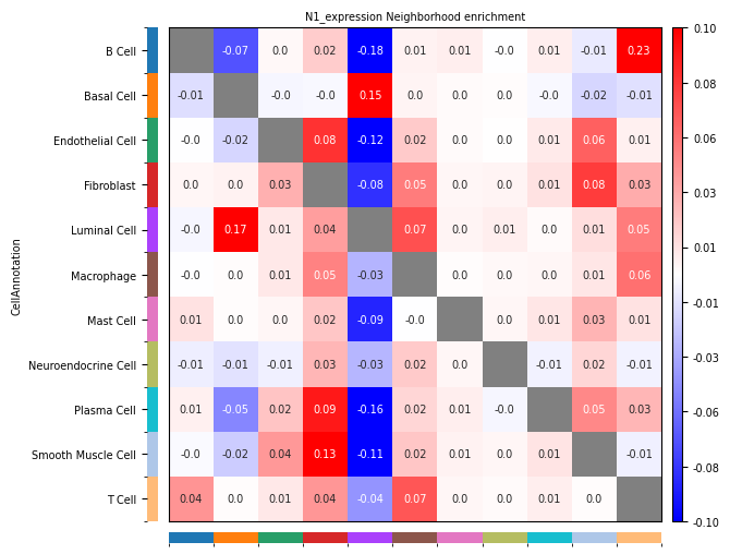
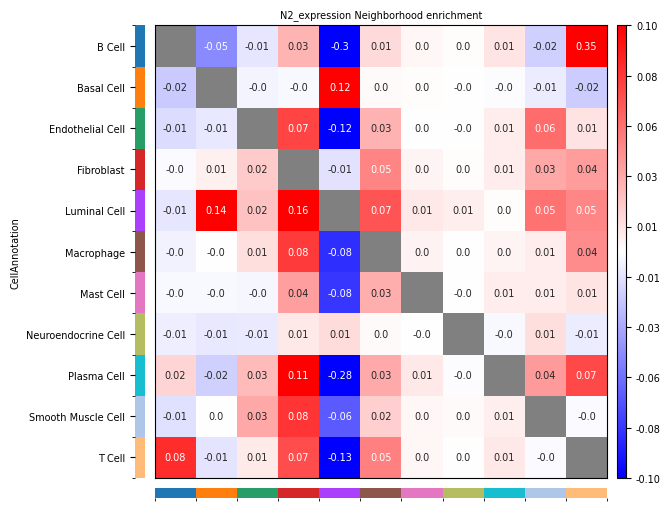
- Row: Source cell type Ci; Column: Target cell type Cj.
- Positive (Observed > Expected): Indicates that cell group Ci and cell group Cj tend to be **enriched** spatially, i.e., more likely to be adjacent. Ci tends to be close to Cj
- Negative (Observed < Expected): Indicates that cell group Ci and cell group Cj tend to be **repelled** spatially, i.e., more likely to be separated. Ci tends to be far from Cj.
- Zero (Observed = Expected): Indicates that the number of connections between cell group Ci and cell group Cj is consistent with random expectation, with no obvious enrichment or repulsion.
Multi-Sample Comparison of Cell Type Colocalization
Compare neighborhood enrichment under different conditions (samples/groups)
cc.gr.diff_nhood_enrichment(
    adata,
    cluster_key=col_celltype,
    condition_key=col_sam,
    library_key=col_group,
    pvalues=True,
    n_jobs=15,
    n_perms=100
)combinations_list = list(combinations(sample_name, 2))
for i in range(len(combinations_list)):
cc.pl.diff_nhood_enrichment(
adata,
cluster_key=col_celltype,
condition_key=col_group,
condition_groups=list(combinations_list[i]),
annotate=True,
figsize=(5,5),
#significance=0.05,
fontsize=5,
save="./"+list(combinations_list[i])[0]+"vs"+list(combinations_list[i])[1]+"_"+col_celltype+"_enrichment_heatmap.png"
)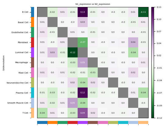
- Row: Source cell type Ci; Column: Target cell type Cj.
- Positive (Observed > Expected): Indicates that in the experimental group (vs pre), cell group Ci and cell group Cj tend to be **enriched** spatially, i.e., more likely to be adjacent.
- Negative (Observed < Expected): Indicates that in the experimental group (vs pre), cell group Ci and cell group Cj tend to be **repelled** spatially, i.e., more likely to be separated.
- Zero (Observed = Expected): Indicates that the number of connections between cell group Ci and cell group Cj is consistent with random expectation, with no obvious enrichment or repulsion.
Result Files
- *_enrichment_heatmap.png/pdf Cell Type Colocalization Plot
References
[1] Varrone M, Tavernari D, Santamaria-Martínez A et al. CellCharter reveals spatial cell niches associated with tissue remodeling and cell plasticity[J]. Nat Genet, 2024, 56: 74–84.
Appendix
.xls, .txt: Result data table files, tab-separated. Unix/Linux/Mac users use less or more commands to view; Windows users use advanced text editors like Notepad++ to view, or open with Microsoft Excel.
.png: Result image files, bitmap, lossless compression.
.pdf: Result image files, vector graphics, can be zoomed in and out without distortion, convenient for users to view and edit, can use Adobe Illustrator for image editing, used for article publication, etc.