Single-Cell Host-Virus Interaction: Correlation Study between Gene Expression Abundance and Viral Load

Author: SeekGene

Time: 7 min

Words: 1.3k words

Updated: 2026-02-27

Reads: 0 times

3' scRNA-seq 5' + Immune Profiling Analysis Guide Correlation Analysis FFPE scRNA-seq Notebooks Spatial-seq scATAC + RNA-seq scFAST-seq

##################################### 
# Select Jupyter script execution environment as copyKAT #
#####################################

library(Seurat)
library(ggplot2)
library(ggpubr)

output

Loading required package: SeuratObject

Loading required package: sp

‘SeuratObject’ was built with package ‘Matrix’ 1.6.4 but the current
version is 1.7.0; it is recomended that you reinstall ‘SeuratObject’ as
the ABI for ‘Matrix’ may have changed


Attaching package: ‘SeuratObject’


The following objects are masked from ‘package:base’:

intersect, t

Gene expression data uses "ESCC Paper Reproduction" - "Large Group Reproduction" data as an example

Read workflow RDS data, relative path data/, absolute path /home/mambauser/data/

# Workflow rds is data/ProcessID/input.rds
obj = readRDS("data/AY1743044870655/input.rds")
head(obj@meta.data)

A data.frame: 6 × 10

	orig.ident	nCount_RNA	nFeature_RNA	Sample	mito	raw_Sample	Tissue	Patient	resolution.0.6_d20	mitorelatedgenes
	<chr>	<dbl>	<int>	<fct>	<dbl>	<chr>	<fct>	<fct>	<fct>	<dbl>
AAACCTGAGATACACA-1_1	SeuratProject	2797	1425	S150T	4.2903	GSE145370_S150T	Tumor	S150	1	3.3249911
AAACCTGAGCTAACTC-1_1	SeuratProject	2790	1349	S150T	1.1470	GSE145370_S150T	Tumor	S150	5	1.0035842
AAACCTGAGGAGCGAG-1_1	SeuratProject	1768	1054	S150T	4.7511	GSE145370_S150T	Tumor	S150	1	4.0158371
AAACCTGAGGGAAACA-1_1	SeuratProject	4455	2017	S150T	2.2896	GSE145370_S150T	Tumor	S150	8	1.8855219
AAACCTGAGTCCCACG-1_1	SeuratProject	1422	861	S150T	0.9845	GSE145370_S150T	Tumor	S150	1	0.7032349
AAACCTGAGTGAACAT-1_1	SeuratProject	2522	1308	S150T	1.7843	GSE145370_S150T	Tumor	S150	4	1.5463918

gene_expression_matrix = Seurat::GetAssayData(object = obj, slot = "counts")
gene_expression_matrix[1:3, 1:3]

output

Warning message:
“The \`slot\` argument of \`GetAssayData()\` is deprecated as of SeuratObject 5.0.0.
ℹ Please use the \`layer\` argument instead.”



3 x 3 sparse Matrix of class "dgCMatrix"
AAACCTGAGATACACA-1_1 AAACCTGAGCTAACTC-1_1 AAACCTGAGGAGCGAG-1_1
MIR1302-2HG . . .
AL627309.1 . . .
AL627309.2 . . .

Viral gene expression data here uses simulated data based on negative binomial distribution

virus_expression = read.delim("sim_virus.matrix")
virus_expression[1:3,1:3]
virus_expression = Matrix::as.matrix(virus_expression)

A data.frame: 3 × 3

	AAACCTGAGATACACA.1_1	AAACCTGAGCTAACTC.1_1	AAACCTGAGGAGCGAG.1_1
	<int>	<int>	<int>
virus-gene1	0	1	0
virus-gene2	0	0	0
virus-gene3	0	0	0

# Construct new object, obtain normalized gene expression data
new_obj = CreateSeuratObject(counts = Matrix::rbind2(gene_expression_matrix, virus_expression))
new_obj = NormalizeData(new_obj)
new_obj$Sample = obj$Sample

output

Normalizing layer: counts

# Obtain viral gene names and host gene names respectively
virus_gene = rownames(new_obj)[grep("^virus", rownames(new_obj))]
host_gene = setdiff(rownames(new_obj), virus_gene)

# Obtain viral gene expression data
virus_data=GetAssayData(new_obj,assay = "RNA", slot = "data")[virus_gene,]
virus_data_sum = colSums(virus_data)

# Obtain host gene expression data
host_data = GetAssayData(obj, slot = "data")[host_gene,]
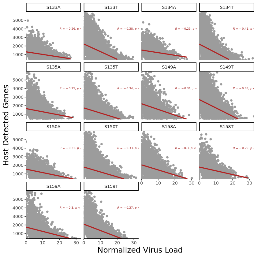
host_gene_num = colSums(host_data != 0)

Definition

Gene Expression Abundance: Number of genes expressed in cells

Viral Load: Sum of normalized viral gene expression values (refer to the article above)

plot_data=data.frame(virus_load = virus_data_sum,
                     host_gene_num = host_gene_num,
                    Sample = new_obj$Sample)
head(plot_data)

A data.frame: 6 × 3

	virus_load	host_gene_num	Sample
	<dbl>	<int>	<fct>
AAACCTGAGATACACA-1_1	2.726585	1425	S150T
AAACCTGAGCTAACTC-1_1	4.249812	1349	S150T
AAACCTGAGGAGCGAG-1_1	8.147058	1054	S150T
AAACCTGAGGGAAACA-1_1	5.170728	2017	S150T
AAACCTGAGTCCCACG-1_1	13.314534	861	S150T
AAACCTGAGTGAACAT-1_1	0.000000	1308	S150T

Plotting

p <- ggplot(plot_data, aes(x = virus_load, y = host_gene_num)) +
  geom_point(color = "#9C9C9C", size = 1.5) +
  geom_smooth(method = "lm", se = TRUE, color = "Firebrick") +  # Add linear fit line
  facet_wrap(~Sample) + # Facet by Sample
  theme_classic() +
  theme(
    axis.title = element_text(size = 15),  # Increase axis font size
    plot.title = element_text(hjust = 0.5, size = 18, face = "bold"),  # Center title
  ) +
  labs(
    x = "Normalized Virus Load", # x-axis title
    y = "Host Detected Genes"# y-axis title
  ) +
  stat_cor(label.x = 20, label.y = 4000, # Position of correlation value
           size = 2, # Correlation value font size
           color = "brown") + # Add correlation coefficient 
    scale_x_continuous(expand = c(0,0)) + # Adjust x-axis range
    scale_y_continuous(expand = c(0,0),limits = range(plot_data$host_gene_num)) # Adjust y-axis range
p

output

\`geom_smooth()\` using formula = 'y ~ x'
Warning message:
“Removed 152 rows containing missing values or values outside the scale range
(\`geom_smooth()\`).”

Save Image

ggsave(p, file = "correlation.png", width = 10, height = 10)

output

\`geom_smooth()\` using formula = 'y ~ x'
Warning message:
“Removed 152 rows containing missing values or values outside the scale range
(\`geom_smooth()\`).”

END