scMethyl + RNA Multi-omics: MethSCAn Differential Methylation Analysis

Author: SeekGene

Time: 25 min

Words: 4.9k words

Updated: 2026-03-18

Reads: 0 times

scMethyl + RNA-seq Notebooks

Module Introduction

This module is developed based on MethSCAn and is designed for single-cell methylation data analysis.

MethSCAn is a powerful suite of command-line tools capable of systematic preprocessing, quality control, variable region detection, and downstream analysis of single-cell methylation data. By detecting genome-wide methylation variations, it achieves the following core analysis goals:

VMR Detection (Variably Methylated Regions): Automatically identifies regions with methylation variation across cells (Variably Methylated Regions, VMRs), which are often associated with cell types, developmental stages, or disease states.
Cell Clustering: Performs clustering of cells based on the methylation feature matrix to effectively distinguish different cell types or cell states, similar to cell clustering analysis in single-cell RNA-seq.
DMR Analysis (Differentially Methylated Regions): Identifies Differentially Methylated Regions (DMRs) between different cell populations to reveal epigenetic heterogeneity.

Input File Preparation

This module supports analysis starting from the compact_data directory. The compact_data directory is typically generated by the following data preprocessing workflow:

Data Preprocessing Workflow

Methylation-aware Mapping and Extraction: Use the allcools analysis pipeline for mapping and methylation site extraction to obtain allc files containing methylation and non-methylation site information.
Format Conversion: Use allc_to_bismarkCov.py to convert allc files to bismark coverage format (.cov files).
Data Preparation: Use methscan prepare to convert .cov files into the efficient compact_data format.

Note:

Although MethSCAn supports allc format input, processing speed is very slow, so it is recommended to convert to bismark coverage format before analysis.
Generally, SeekSoul Online has completed the allc_to_bismarkCov.py and methscan prepare steps by default, so you can directly use the existing compact_data directory for analysis.

File Structure Example

The compact_data directory structure is as follows:

text

compact_data/
├── chr1.npz
├── chr2.npz
├── chr3.npz
├── ...
├── chrX.npz
├── column_header.txt
└── cell_stats.csv

MethSCAn Analysis Workflow

Script Description: The following code serves as an initialization example for the MethSCAn analysis workflow, including environment configuration, path settings, and helper function definitions for subsequent steps.

options(warn = -1)
# Load required R packages
suppressPackageStartupMessages({
  library(ggplot2)      # For data visualization
  library(dplyr)        # For data manipulation
  library(readr)        # For reading CSV files
  library(tidyverse)    # Data tidying and visualization suite
  library(data.table)   # Efficient data reading and processing
  library(irlba)        # For iterative PCA (imputing missing values)
  library(Seurat)       # Single-cell analysis tool (version v5)
  library(Matrix)       # Sparse matrix processing
})

# --- Input Parameter Configuration ---

## methscan_path: MethSCAn command path
# If methscan is in system PATH, set to NULL
# If methscan is in a different environment, specify full path
methscan_path <- "/jp_envs/envs/methscan/bin/methscan"

## outdir: Result output directory
outdir <- "./DMRs"
# Create output directory (if it doesn't exist)
dir.create(outdir, recursive = TRUE, showWarnings = FALSE)

## compact_data_dir: compact_data directory (generated by methscan prepare)
compact_data_dir <- file.path("../../data/AY1768874914782/methylation/demoWTJW969-task-1/WTJW969/methscan/compact_data")

## n_threads: Number of threads for parallel computing
# Note: MethSCAn automatically detects the system's maximum thread count. Error occurs if n_threads is set higher than system limit.
# Recommended to set less than or equal to available CPU cores.
n_threads <- 8

# Define function: Call MethSCAn command in R
run_methscan <- function(command, args = character(), methscan_path = NULL) {
  # Determine command path: Prioritize argument, then global variable, finally system PATH
  if (is.null(methscan_path) && exists("methscan_path", envir = .GlobalEnv)) {
    methscan_path <- get("methscan_path", envir = .GlobalEnv)
  }
  cmd <- if (is.null(methscan_path)) "methscan" else methscan_path
  
  cat("Executing:", cmd, command, paste(args, collapse = " "), "\n")
  
  # Create temp files to capture stdout and stderr
  stdout_file <- tempfile()
  stderr_file <- tempfile()
  
  # Execute command, capture output
  result <- system2(
    cmd, 
    args = c(command, args), 
    wait = TRUE,
    stdout = stdout_file,
    stderr = stderr_file
  )
  
  return(invisible(result))
}

Key Parameter Settings

This section provides a centralized explanation of the key parameters involved in the MethSCAn analysis workflow. These parameters will be called in subsequent steps such as methscan filter, methscan scan, methscan matrix, and methscan diff, used to control key behaviors including cell quality filtering, variably methylated region detection, and differential analysis.

`methscan filter` Parameters

For detailed explanations and recommended values of key parameters involved in low-quality cell filtering (such as min_sites, min_meth, max_meth, etc.), please refer to the parameter table before the filtering execution code in Section 3.3.2.

`methscan diff` Parameters

Key parameters involved in Differentially Methylated Regions (DMR) analysis for comparing two clusters are as follows:

Parameter Name	Meaning	Default Value	Detailed Description
`min_cells`	Minimum Cell Count Requirement	6	Quality Control (QC) Parameter. Requires that each genomic region must have sequencing coverage in at least this number of cells in each comparison group to be included in the differential analysis. For example, setting it to 6 means only regions with coverage in at least 6 cells per group will be considered for differential testing. Note: This parameter helps filter out regions with insufficient coverage, improving the reliability of DMR detection. If the number of cells in a group is small, this value can be appropriately lowered, but it may increase false positives.

`threads` Parameter (General Parameter)

Number of parallel computing threads used to accelerate computationally intensive steps (such as scan, matrix, diff).

Parameter Name	Meaning	Default/Recommended Value	Detailed Description
`threads`	Parallel Computing Threads	8	Performance Optimization Parameter. Used to accelerate computationally intensive steps (such as `scan`, `matrix`, `diff`). It is recommended to set based on system resources, usually set to the number of available CPU cores. Important: MethSCAn automatically detects the system's maximum thread count. The program will report an error if `threads` is set higher than the system's maximum thread count. Therefore, it is recommended to set `threads` to a value less than or equal to the number of available CPU cores.

Best Practice Recommendations

Selection of methscan filter Parameters:
Quality Assessment: It is strongly recommended to run the quality assessment step first (see Section 3.3.1), visualize the distribution of methylation site counts and global methylation percentages per cell, identify outliers based on visualization results, and finally determine the values for min_sites, min_meth, and max_meth.
Strategy for min_sites: If too few cells are retained, min_sites can be appropriately lowered (e.g., to 20000), but this may increase noise. If data quality is very good, the threshold can be raised to obtain more reliable results.
Global Methylation Percentage Thresholds (min_meth and max_meth): Normal methylation levels for different species:
- Mouse: Typically 70-80%.
- Human: Typically 60-70%.
Computing Resources:
methscan scan, matrix, diff: Default use of 8c64g resources. The entire run usually takes 1-2 hours. If using resources on SeekSoul Online, it is recommended to set the extended time to 3 hours.
About the min_cells Parameter in DMR Analysis:
Default Value: 6 cells/group
Function: Ensures that there is a sufficient number of cells with sequencing coverage for a region in each comparison group before differential analysis is performed. This helps improve the statistical power and reliability of DMR detection.
Empirical Suggestion: Based on experience, valid DMRs with significant p-values can be obtained when the number of cells in both clusters being compared is greater than 200. If the number is too small, significant results may not be obtained. When the cell count is low, this parameter can be lowered for testing.

# --- Note: methscan prepare has been completed on the cloud platform, results can be used directly ---
# Uncomment below if re-run is needed

# # Check if input directory exists
# if (!dir.exists(input_cov_dir)) {
#   stop("Input directory does not exist: ", input_cov_dir, 
#        "\nPlease run allc_to_bismarkCov.py to convert data first")
# }
# 
# # Get all coverage files
# cov_files <- list.files(input_cov_dir, full.names = TRUE, pattern = "\\.cov$")
# if (length(cov_files) == 0) {
#   stop("No .cov files found in ", input_cov_dir)
# }
# 
# cat("Found ", length(cov_files), " coverage files\n")
# 
# # Prepare output directory
# compact_data_dir <- file.path(outdir, "compact_data")
# if (!dir.exists(compact_data_dir)) {
#   dir.create(compact_data_dir, recursive = TRUE)
# }
# 
# # Execute methscan prepare
# run_methscan(
#   command = "prepare",
#   args = c(cov_files, compact_data_dir)
# )

# Directly use existing compact_data directory
if (!dir.exists(compact_data_dir)) {
  stop("compact_data directory does not exist: ", compact_data_dir, 
       "\nPlease ensure methscan prepare step is completed on the cloud platform")
}
cat("✓ Using existing compact_data directory:", compact_data_dir, "\n")

output

✓ Using existing compact_data directory: ../../data/AY1768874914782/methylation/demoWTJW969-task-1/WTJW969/methscan/compact_data

Quality Assessment and Filtering of Low-Quality Cells

Before filtering, it is recommended to assess cell quality first and determine filtering parameters based on visualization results.

Read Cell Statistics and Visualize Quality Metrics

# Read cell_stats.csv file
cell_stats_path <- file.path(compact_data_dir,  "cell_stats.csv")

cell_stats <- read_csv(cell_stats_path)

#if (file.exists(cell_stats_path)) {
#  cell_stats <- read_csv(cell_stats_path)
#  cat("Successfully read cell statistics, total", nrow(cell_stats), "cells\n")
#  head(cell_stats)
#} else {
#  stop("cell_stats.csv file not found, please check if path is correct")
#}

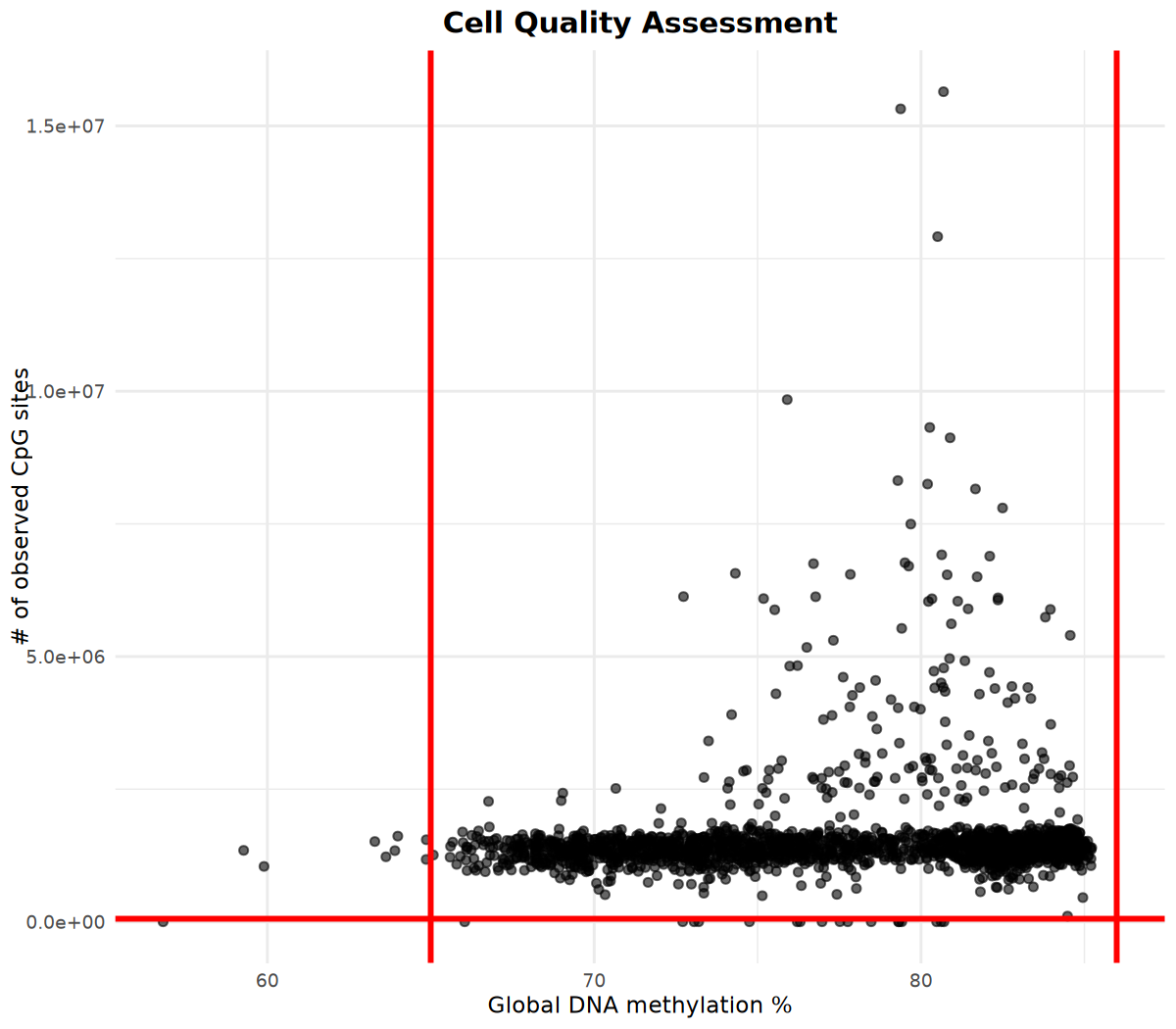
# Visualize methylation site counts and global methylation percentage
# Determine filtering parameters based on visualization results

options(repr.plot.width = 8, repr.plot.height = 7, repr.plot.res = 150)
p <- cell_stats %>% 
  ggplot(aes(x = global_meth_frac * 100, y = n_obs)) +
  geom_point(alpha = 0.6) +
  # Add red vertical lines at x=65 and x=86 (example thresholds)
  geom_vline(xintercept = c(65, 86), color = "red", linetype = "solid", linewidth = 1) +
  # Add red horizontal line at y=60000 (example threshold)
  geom_hline(yintercept = 60000, color = "red", linetype = "solid", linewidth = 1) +
  labs(
    x = "Global DNA methylation %", 
    y = "# of observed CpG sites",
    title = "Cell Quality Assessment"
  ) +
  theme_minimal() +
  theme(
    plot.title = element_text(hjust = 0.5, size = 14, face = "bold")
  )

print(p)

output

Rows: 2196 Columns: 4
── Column specification ────────────────────────────────────────────────────────
Delimiter: ","
chr (1): cell_name
dbl (3): n_obs, n_meth, global_meth_frac

ℹ Use \`spec()\` to retrieve the full column specification for this data.
ℹ Specify the column types or set \`show_col_types = FALSE\` to quiet this message.

Filter based on visualization results

Based on the visualization results above, determine filtering parameters and perform cell filtering:

methscan filter Key Parameters:

Parameter Name	Meaning	Default/Recommended Value	Detailed Description
`min_sites`	Minimum Observed Methylation Sites	25000-60000	Quality Control (QC) Parameter. Requires that each cell must have observed methylation sites greater than this value. Used to remove low-quality cells with insufficient sequencing depth or unable to accurately infer methylation state. Note: The threshold depends on sequencing depth; the higher the depth, the higher the threshold can be set.
`min_meth`	Minimum Global Methylation Percentage	60-70	Quality Control (QC) Parameter. Requires that each cell's global methylation percentage must be greater than this value. Used to remove abnormal cells potentially due to incomplete bisulfite conversion or technical issues. Note: Normal methylation levels vary greatly between different species and cell types (e.g., Mouse is typically 70-80%, Human is 60-70%).
`max_meth`	Maximum Global Methylation Percentage	70-85	Quality Control (QC) Parameter. Requires that each cell's global methylation percentage must be less than this value. Used to remove abnormal cells with excessively high methylation due to technical issues. Note: Normal methylation levels vary greatly between different species and cell types; please set a reasonable threshold range based on actual data.
`threads`	Parallel Computing Threads	8	Used to accelerate computationally intensive steps (such as `scan`, `matrix`). It is recommended to set based on system resources, usually set to the number of available CPU cores.

# Filtering parameters (please adjust based on QC results)
min_sites <- 60000    # Minimum observed methylation sites
min_meth <- 65       # Minimum global methylation percentage
max_meth <- 86        # Maximum global methylation percentage

# Prepare output directory
filtered_data_dir <- file.path(outdir, "filtered_data")
if (!dir.exists(filtered_data_dir)) {
  dir.create(filtered_data_dir, recursive = TRUE)
}

# Execute methscan filter
run_methscan(
  command = "filter",
  args = c(
    "--min-sites", min_sites,
    "--min-meth", min_meth,
    "--max-meth", max_meth,
    compact_data_dir,
    filtered_data_dir
  )
)

output

Executing: /jp_envs/envs/methscan/bin/methscan filter --min-sites 60000 --min-meth 65 --max-meth 86 ../../data/AY1768874914782/methylation/demoWTJW969-task-1/WTJW969/methscan/compact_data ./DMRs/filtered_data

Data Smoothing: methscan smooth

Before VMR/DMR detection, methylation data needs to be smoothed. methscan smooth treats all single cells as a pseudo-bulk sample to calculate genome-wide smoothed average methylation. This information is required for VMR detection and subsequent methylation matrix generation.

Output: Output files are located in the ${outdir}/filtered_data/smoothed directory.

# Execute methscan smooth
run_methscan(
  command = "smooth",
  args = filtered_data_dir
)

output

Executing: /jp_envs/envs/methscan/bin/methscan smooth ./DMRs/filtered_data

Detecting VMRs: methscan scan

Detect Variably Methylated Regions (VMRs). methscan scan automatically identifies regions with methylation variation across cells.

Output: Outputs a BED format file containing genomic coordinates and methylation variance of VMRs.

Alternative: If you are interested in specific genomic regions (such as promoters, gene bodies), you can also directly provide a BED file, skip the scan step, and proceed directly to methscan matrix to analyze these regions.

# VMR output file
vmr_bed_file <- file.path(outdir, "VMRs.bed")

# Execute methscan scan
result <- run_methscan(
  command = "scan",
  args = c(
    "--threads", n_threads,
    filtered_data_dir,
    vmr_bed_file
  )
)

output

Executing: /jp_envs/envs/methscan/bin/methscan scan --threads 8 ./DMRs/filtered_data ./DMRs/VMRs.bed

Generating VMR Matrix: methscan matrix

Generate a methylation matrix based on VMR regions for subsequent clustering analysis.

Output File Description:

The output directory VMR_matrix contains the following files:

Filename	Description
`mean_shrunken_residuals.csv.gz`	Mean Shrunken Residuals Matrix (recommended for downstream analysis). Less affected by random coverage variations, making it more suitable for dimensionality reduction and clustering analysis.
`methylation_fractions.csv.gz`	Methylation Fraction Matrix. The methylation fraction (between 0-1) for each region, representing the average methylation level of that region.
`methylated_sites.csv.gz`	Methylated Sites Matrix (Numerator). The number of methylated CpG sites in each region.
`total_sites.csv.gz`	Total Sites Matrix (Denominator). The total number of CpG sites with sequencing coverage in each region.

Matrix Characteristics:

The matrix contains a large number of missing values: due to low single-cell sequencing coverage, many regions may lack sequencing reads.
Methylation values often appear as fractions with small denominators (e.g., 1/1, 2/2, 1/3, etc.), which is a typical characteristic of single-cell methylation data.
The output directory also contains the number of methylated CpG sites and the number of CpG sites with sequencing coverage for each region (i.e., the numerator and denominator of the methylation fraction).

# VMR matrix output directory
vmr_matrix_dir <- file.path(outdir, "VMR_matrix")

# Execute methscan matrix
result <- run_methscan(
  command = "matrix",
  args = c(
    "--threads", n_threads,
    vmr_bed_file,
    filtered_data_dir,
    vmr_matrix_dir
  )
)

# Check if output files are generated
if (result == 0 && dir.exists(vmr_matrix_dir)) {
  expected_files <- c(
    "mean_shrunken_residuals.csv.gz",
    "methylation_fractions.csv.gz",
    "methylated_sites.csv.gz",
    "total_sites.csv.gz"
  )
  existing_files <- list.files(vmr_matrix_dir)
  found_files <- expected_files[expected_files %in% existing_files]
  
  if (length(found_files) > 0) {
    cat("✓ VMR matrix files generated:\n")
    for (f in found_files) {
      file_path <- file.path(vmr_matrix_dir, f)
      file_size <- file.info(file_path)$size / 1024 / 1024  # MB
      cat("  -", f, sprintf("(%.2f MB)\n", file_size))
    }
  } else {
    warning("Warning: Expected output files not found, please check output directory: ", vmr_matrix_dir)
  }
} else if (result != 0) {
  stop("methscan matrix execution failed, please check the error message above")
}

output

Executing: /jp_envs/envs/methscan/bin/methscan matrix --threads 8 ./DMRs/VMRs.bed ./DMRs/filtered_data ./DMRs/VMR_matrix
✓ VMR matrix files generated:
- mean_shrunken_residuals.csv.gz (291.34 MB)
- methylation_fractions.csv.gz (60.59 MB)
- methylated_sites.csv.gz (43.48 MB)
- total_sites.csv.gz (56.35 MB)

Clustering Analysis Based on VMRs

This section will use Seurat to perform dimensionality reduction and clustering analysis on the VMR matrix.

Read VMR Matrix

# Read compressed file using fread
# Use configured outdir variable
vmr_matrix_path <- file.path(outdir, "VMR_matrix", "mean_shrunken_residuals.csv.gz")

if (file.exists(vmr_matrix_path)) {
  cat("Reading VMR matrix...\n")
  meth_mtx <- fread(vmr_matrix_path)
  cat("Matrix dimensions:", nrow(meth_mtx), "rows (cells) x", ncol(meth_mtx) - 1, "columns (VMR regions)\n")
  
  # Set first column as row names and convert to matrix
  row_names <- meth_mtx[[1]]
  meth_mtx <- as.matrix(meth_mtx[, -1])
  rownames(meth_mtx) <- row_names
  
  cat("Matrix conversion completed!\n")
  cat("Missing value proportion:", round(mean(is.na(meth_mtx)) * 100, 2), "%\n")
} else {
  stop("VMR matrix file not found, please check if path is correct")
}

output

Reading VMR matrix...n Matrix dimensions: 2170 rows (cells) x 106967 columns (VMR regions)
Matrix conversion completed!
Missing value proportion: 75.31 %

Iterative PCA for Imputing Missing Values

The methylation matrix is similar to the count matrix in single-cell RNA-seq, but a major difference is that it contains a large number of missing values. This is because the sequencing coverage for each single cell is low, meaning many genomic regions do not receive any sequencing reads.

To address this issue, we use an iterative PCA method to impute missing values: missing values are first replaced with 0 (as an initial guess), then PCA is run on the imputed matrix. The values predicted by PCA are used to replace the previously filled 0s, and this process is repeated until the imputed values converge (change is minimal).

This method uses iterative optimization to more accurately estimate missing methylation values, providing more complete data for subsequent dimensionality reduction and clustering analysis.

# Define function for iterative PCA imputation
prcomp_iterative <- function(x, n = 15, n_iter = 50, min_gain = 0.001, ...) {
  mse <- rep(NA, n_iter)
  na_loc <- is.na(x)
  x[na_loc] <- 0  # zero is our first guess

  for (i in 1:n_iter) {
    prev_imp <- x[na_loc]  # what we imputed in the previous round
    # PCA on the imputed matrix
    pr <- prcomp_irlba(x, center = F, scale. = F, n = n, ...)
    # impute missing values with PCA
    new_imp <- (pr$x %*% t(pr$rotation))[na_loc]
    x[na_loc] <- new_imp
    # compare our new imputed values to the ones from the previous round
    mse[i] <- mean((prev_imp - new_imp) ^ 2)
    # if the values didn't change a lot, terminate the iteration
    gain <- mse[i] / max(mse, na.rm = T)
    if (gain < min_gain) {
      message(paste(c("\n\nTerminated after ", i, " iterations.")))
      break
    }
  }
  message(paste(c("\n\nTerminated after ", i, " iterations. Gain: ", round(gain, 6))))
  pr$mse_iter <- mse[1:i]
  list(pr = pr, imputed_matrix = x)
}

cat("Executing iterative PCA for missing value imputation...\n")
result_residual <- meth_mtx %>% 
  scale(center = T, scale = F) %>% 
  prcomp_iterative(n = 15)

# Extract imputed residual matrix
residual_mtx_imputed <- result_residual$imputed_matrix
cat("Missing value imputation completed!\n")

output

Executing iterative PCA for missing value imputation...n

Terminated after 32 iterations.

Terminated after 32 iterations. Gain: 0.000974

Missing value imputation completed!

Create Seurat Object

Description: The matrix after imputing missing values using the residual matrix (residual_mtx_imputed) is used as input for the Seurat object. In the Seurat object, the counts, data, and scale.data matrices all use the same imputed residual matrix. Note: Subsequent PCA, dimensionality reduction, and clustering analysis actually use the scale.data matrix.

# Create Seurat object using the imputed residual matrix
# counts, data, and scale.data all use the same imputed residual matrix
seurat_obj <- CreateSeuratObject(
    counts = as(t(residual_mtx_imputed), "sparseMatrix"),
    project = "MethSCAn",
    assay = "VMR"
)
# Set data and scale.data to be the same matrix as counts
# Note: Subsequent PCA, dimensionality reduction, and clustering analysis actually use the scale.data matrix
seurat_obj@assays$VMR@data <- seurat_obj@assays$VMR@counts
seurat_obj@assays$VMR@scale.data <- as.matrix(seurat_obj@assays$VMR@counts)

PCA, UMAP Dimensionality Reduction and Clustering

# 1. PCA Dimensionality Reduction
# Use Seurat's RunPCA function
# This automatically reads data from the scale.data layer and calculates PCA
n_pcs = 30
seurat_obj <- RunPCA(
    seurat_obj,
    features = rownames(seurat_obj),  # Use all VMRs
    npcs = n_pcs,  # Calculate top 30 principal components
    assay = "VMR",
    verbose = FALSE
)

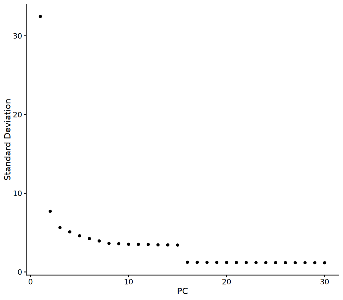
# Visualize Elbow Plot to determine the number of principal components to use
ElbowPlot(seurat_obj, ndims = 30)

# 2. Determine the number of principal components to use based on Elbow Plot
# You can adjust this parameter based on the Elbow Plot results
n_pcs_use <- 10

# 3. UMAP Dimensionality Reduction
seurat_obj <- RunUMAP(seurat_obj, dims = 1:n_pcs_use, reduction = "pca")
cat("UMAP dimensionality reduction completed!\n")

# 4. Construct KNN Graph
seurat_obj <- FindNeighbors(seurat_obj, dims = 1:n_pcs_use, reduction = "pca")
cat("KNN graph construction completed!\n")

# 5. Clustering (resolution parameter can be adjusted; larger values yield more clusters)
seurat_obj <- FindClusters(seurat_obj, resolution = 0.5)
cat("Clustering completed!\n")

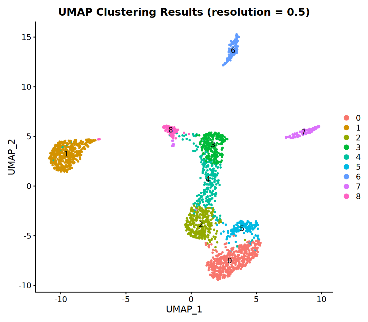
# 6. Visualize Clustering Results
DimPlot(seurat_obj, group.by = 'VMR_snn_res.0.5', label = TRUE) + 
  ggtitle("UMAP Clustering Results (resolution = 0.5)")

output

18:16:32 UMAP embedding parameters a = 0.9922 b = 1.112

18:16:32 Read 2170 rows and found 10 numeric columns

18:16:32 Using Annoy for neighbor search, n_neighbors = 30

18:16:32 Building Annoy index with metric = cosine, n_trees = 50

0% 10 20 30 40 50 60 70 80 90 100%

[----|----|----|----|----|----|----|----|----|----|

*
*
*
*
*
*
*
*
*
*
*
*
*
*
*
*
*
*
*
*
*
*
*
*
*
*
*
*
*
*
*
*
*
*
*
*
*
*
*
*
*
*
*
*
*
*
*
*
*
*
|

18:16:32 Writing NN index file to temp file /tmp/Rtmp6mqHG9/filecfb7f2cfded

18:16:32 Searching Annoy index using 1 thread, search_k = 3000

18:16:33 Annoy recall = 100%

18:16:34 Commencing smooth kNN distance calibration using 1 thread
with target n_neighbors = 30

18:16:34 Initializing from normalized Laplacian + noise (using irlba)

18:16:34 Commencing optimization for 500 epochs, with 92182 positive edges

18:16:34 Using rng type: pcg

18:16:37 Optimization finished

UMAP dimensionality reduction completed!

Computing nearest neighbor graph

Computing SNN

KNN graph construction completed!
Modularity Optimizer version 1.3.0 by Ludo Waltman and Nees Jan van Eck

Number of nodes: 2170
Number of edges: 76302

Running Louvain algorithm...n Maximum modularity in 10 random starts: 0.9031
Number of communities: 9
Elapsed time: 0 seconds
Clustering completed!

Save Results

# Save Seurat Object
output_file <- "MethSCAn.rds"
saveRDS(seurat_obj, file = output_file)

clust_tbl <- seurat_obj@meta.data
clust_tbl$cell <- row.names(clust_tbl)
clust_tbl %>%
  mutate(cell_group = case_when(
    seurat_clusters == "0" ~ "-",
    seurat_clusters == "1" ~ "1",
    seurat_clusters == "2" ~ "2",
    seurat_clusters == "3" ~ "-",
    seurat_clusters == "4" ~ "-",
    seurat_clusters == "5" ~ "-",
    seurat_clusters == "6" ~ "-",
    seurat_clusters == "7" ~ "-",
    seurat_clusters == "8" ~ "-"    
  )) %>% 
  dplyr::select(cell, cell_group) %>%
  write_csv("cell_groups.csv", col_names=F)

Differentially Methylated Region Analysis: methscan diff

Differentially Methylated Region (DMR) analysis is used to compare differentially methylated regions between cells under two different conditions, which can be two clusters, two cell types, or other conditions. It is recommended to perform DMR analysis based on clustering results after completing clustering analysis.

Input File Preparation

Input Files:

Data Directory: filtered_data directory (must have run methscan smooth).
Cell Groups File (cell_groups_file): CSV format, where the first column is the cell name (cell barcode) and the second column is the group label. Label rules: group_A and group_B represent the two groups to be compared, and - represents other cells not involved in the comparison.

File Format Example:

csv

cell_01,-
cell_02,-
cell_03,-
cell_04,group_A
cell_05,group_A
cell_06,group_A
cell_07,group_B
cell_08,group_B
cell_09,group_B

# Cell groups file (for DMR analysis)
cell_groups_file <- "cell_groups.csv"  # Please modify according to actual situation

# DMR output file
dmr_bed_file <- file.path(outdir, "DMRs.bed")

# Check if cell groups file exists
if (file.exists(cell_groups_file)) {
  # Execute methscan diff
  run_methscan(
    command = "diff",
    args = c(
      "--threads", n_threads,
      filtered_data_dir,
      cell_groups_file,
      dmr_bed_file
    )
  )
} else {
  warning("Cell groups file does not exist: ", cell_groups_file, 
          "\nSkipping DMR analysis. To perform DMR analysis, please prepare the cell groups file first.")
}

output

Executing: /jp_envs/envs/methscan/bin/methscan diff --threads 8 ./DMRs/filtered_data cell_groups.csv ./DMRs/DMRs.bed

Output File Format Description

Output File: DMRs.bed is a BED format file containing the following columns:

Col No.	Col Name	Meaning	Example Value
1	`chromosome`	Chromosome name	17
2	`DMR_start`	DMR start position (genomic coordinate)	58270529
3	`DMR_end`	DMR end position (genomic coordinate)	58285529
4	`t_statistic`	Welch's t-test statistic	-12.85232790631932
5	`n_sites`	Total number of methylation sites in the region (CpG count)	561
6	`n_cells_group1`	Number of cells with coverage in Group 1	150
7	`n_cells_group2`	Number of cells with coverage in Group 2	66
8	`meth_frac_group1`	Average methylation level of Group 1 (0–1)	0.3396857458943857
9	`meth_frac_group2`	Average methylation level of Group 2 (0–1)	0.8429240842342447
10	`low_group_label`	Label of the group with lower methylation level	group_1
11	`p`	Raw p-value (unadjusted)	0.0
12	`adjusted_p`	Adjusted p-value (FDR, Benjamini-Hochberg method)	0.0

Result Interpretation: The low_group_label column indicates the group with lower methylation levels. The adjusted_p column contains p-values corrected for multiple testing (suggest filtering for adjusted_p < 0.05). The sign of t_statistic indicates the direction of difference (negative values indicate lower methylation in group_1, positive values indicate higher methylation in group_1).

Generate Significant Differentially Methylated Region Files

Based on the DMRs.bed file, filter significant DMRs (adjusted_p < 0.05) and generate two BED files grouped by low_group_label.

Input:

DMRs.bed: DMR detection result file.

Output:

Generate two significant DMR BED files based on the value of low_group_label:

DMRs_significant_group_A.bed: Regions with significantly lower methylation in group_A.
DMRs_significant_group_B.bed: Regions with significantly lower methylation in group_B.

Each file contains three columns (chromosome, start, end), where chromosome names have the "chr" prefix automatically added (if the original value is a number or X/Y).

Note: Only significant difference regions with adjusted_p < 0.05 are retained. The "chr" prefix is automatically added to numeric and sex chromosomes (if not already present). Rows where low_group_label is empty or "-" are skipped.

# Generate significant DMR files (grouped by low_group_label, adjusted_p < 0.05)
# Add "chr" prefix to autosomes (numbers) and sex chromosomes (X/Y)
# Check if DMRs.bed file exists
if (file.exists(dmr_bed_file)) {
  cat("Starting generation of significant DMR files...\n")
  
  # Construct awk command
  awk_script <- sprintf('
BEGIN {
    outdir = "%s"
}
# Skip header or empty lines
NR == 1 && $1 ~ /^chromosome|^#/ { next }
NF < 12 { next }
# Filter rows with adjusted_p < 0.05
$12 < 0.05 {
    # Get low_group_label (column 10) as filename
    group_label = $10
    if (group_label == "" || group_label == "-") next
    
    # Handle chromosome names: if numeric or X/Y, add "chr" prefix
    chrom = $1
    if (chrom ~ /^[0-9]+$/ || chrom ~ /^[XY]$/) {
        chrom = "chr" chrom
    }
    
    # Construct output filename
    output_file = outdir "/DMRs_significant_" group_label ".bed"
    
    # Output first 3 columns (chromosome, start, end) to corresponding file
    print chrom "\\t" $2 "\\t" $3 > output_file
}
END {
    print "Processing complete! Significant DMR files generated."
}
', outdir)
  
  # Execute awk command in R
  awk_cmd <- paste("awk -F'\\t'", shQuote(awk_script), shQuote(dmr_bed_file))
  result <- system(awk_cmd, intern = TRUE)
  
  # Display output
  cat(paste(result, collapse = "\n"), "\n")
  
  # Check generated files
  significant_files <- list.files(
    path = outdir,
    pattern = "^DMRs_significant_.*\\.bed$",
    full.names = TRUE
  )
  
  if (length(significant_files) > 0) {
    cat("\nGenerated significant DMR files:\n")
    for (f in significant_files) {
      n_lines <- length(readLines(f, warn = FALSE))
      cat("  -", basename(f), " (", n_lines, " regions)\n", sep = "")
    }
  } else {
    warning("No significant DMR files found")
  }
} else {
  warning("DMRs.bed file does not exist: ", dmr_bed_file, 
          "\nPlease run methscan diff command first")
}

output

Starting generation of significant DMR files...n Processing complete! Significant DMR files generated.

Generated significant DMR files:
-DMRs_significant_1.bed (23909 regions)
-DMRs_significant_2.bed (30152 regions)

scMethyl + RNA Multi-omics: MethSCAn Differential Methylation Analysis ​

Module Introduction ​

Input File Preparation ​

Data Preprocessing Workflow ​

File Structure Example ​

MethSCAn Analysis Workflow ​

Key Parameter Settings ​

methscan filter Parameters ​

methscan diff Parameters ​

threads Parameter (General Parameter) ​

Best Practice Recommendations ​

Quality Assessment and Filtering of Low-Quality Cells ​

Read Cell Statistics and Visualize Quality Metrics ​

Filter based on visualization results ​

Data Smoothing: methscan smooth ​

Detecting VMRs: methscan scan ​

Generating VMR Matrix: methscan matrix ​

Clustering Analysis Based on VMRs ​

Read VMR Matrix ​

Iterative PCA for Imputing Missing Values ​

Create Seurat Object ​

PCA, UMAP Dimensionality Reduction and Clustering ​

Save Results ​

Differentially Methylated Region Analysis: methscan diff ​

Input File Preparation ​

Output File Format Description ​

Generate Significant Differentially Methylated Region Files ​

scMethyl + RNA Multi-omics: MethSCAn Differential Methylation Analysis

Module Introduction

Input File Preparation

Data Preprocessing Workflow

File Structure Example

MethSCAn Analysis Workflow

Key Parameter Settings

`methscan filter` Parameters

`methscan diff` Parameters

`threads` Parameter (General Parameter)

Best Practice Recommendations

Quality Assessment and Filtering of Low-Quality Cells

Read Cell Statistics and Visualize Quality Metrics

Filter based on visualization results

Data Smoothing: methscan smooth

Detecting VMRs: methscan scan

Generating VMR Matrix: methscan matrix

Clustering Analysis Based on VMRs

Read VMR Matrix

Iterative PCA for Imputing Missing Values

Create Seurat Object

PCA, UMAP Dimensionality Reduction and Clustering

Save Results

Differentially Methylated Region Analysis: methscan diff

Input File Preparation

Output File Format Description

Generate Significant Differentially Methylated Region Files