SeekSpace Advanced Analysis: Cell Density and Co-localization Based on scider
Load Data
Execution Environment Selection: TumorBoundary
scider is an R package that provides analysis and visualization functions for spatial transcriptomics. The analysis is based on SpatialExperiment objects and can be integrated into various spatial transcriptomics-related packages in Bioconductor. The analysis mainly includes:
- Specific cell density distribution plots
- Cell co-localization
- Automatic detection of Regions of Interest (ROI)
- Specific cell contour plots and cell composition within each contour
scider is a user-friendly R package that provides functionality to model global cell density in spatial transcriptomics data slides. All functions in this package are built on SpatialExperiment objects and can be integrated into various spatial transcriptomics-related packages in Bioconductor. After density modeling, the package allows for multiple downstream analyses, including co-localization analysis, boundary detection analysis, and differential density analysis. scider implements the function of analyzing spatial transcriptomics data with cell type annotations through density estimation for cell type correlation and real distance for cell type co-localization. Features include density estimation, statistical modeling, and visualization.
Functionality to model global cell density in spatial transcriptomics data slides. All functions in this package are built on SpatialExperiment objects and can be integrated into various spatial transcriptomics-related packages in Bioconductor. The package can also perform multiple downstream analyses, including co-localization analysis, boundary detection analysis, and differential density analysis.
The data mainly requires an expression matrix and spatial coordinates. You can directly read three matrix files and a spatial coordinate file, or extract them from an rds file.
expr_matrix <- Read10X('/PROJ2/FLOAT/weichendan/seekspace/WTH1092/demo_WTH1092/Outs/WTH1092_filtered_feature_bc_matrix/')dim(expr_matrix)
expr_matrix[1:5,1:5]- 32285
- 32758
5 x 5 sparse Matrix of class "dgCMatrix"
        AACAGGGTACTGAGGCTAAGGCACTAT AAGCGAGTACATGCAGTGCTCTGCTTC
Xkr4                              .                           .
Gm1992                            .                           .
Gm19938                           .                           .
Gm37381                           .                           .
Rp1                               .                           .
        AAGCGTTTACGTTCTACAGCGACGGAT AAGTCGTCGACTCTAGAGCTCTGCTTC
Xkr4                              .                           .
Gm1992                            .                           .
Gm19938                           .                           .
Gm37381                           .                           .
Rp1                               .                           .
        AATGCCATACGCAGGTTCTAAGTACGA
Xkr4                              .
Gm1992                            .
Gm19938                           .
Gm37381                           .
Rp1                               .
spatial_coords <- read.table("/PROJ2/FLOAT/weichendan/seekspace/WTH1092/demo_WTH1092/Outs/WTH1092_filtered_feature_bc_matrix/cell_locations.tsv.gz",header=T,row.names=1)
colnames(spatial_coords) <- c("spatial_1","spatial_2")
spatial_coords <- spatial_coords[colnames(expr_matrix),]
spatial_coords <- as.matrix(spatial_coords)dim(spatial_coords)
head(spatial_coords)- 32758
- 2
| spatial_1 | spatial_2 | |
|---|---|---|
| AACAGGGTACTGAGGCTAAGGCACTAT | 35374 | 4592 |
| AAGCGAGTACATGCAGTGCTCTGCTTC | 37923 | 17104 |
| AAGCGTTTACGTTCTACAGCGACGGAT | 35866 | 18687 |
| AAGTCGTCGACTCTAGAGCTCTGCTTC | 34480 | 17330 |
| AATGCCATACGCAGGTTCTAAGTACGA | 44055 | 14412 |
| ACAGAAATACGGCAGTCTTCTGCGCTC | 15652 | 6521 |
Create SpatialExperiment Object
scider analysis is based on SpatialExperiment objects. After constructing the SpatialExperiment object, various annotations and clustering information for cells can be added.
spe <- SpatialExperiment(
  assays = list(counts = expr_matrix),          # Expression matrix, usually named "counts"
  spatialCoords = spatial_coords                # Spatial coordinates
)spedim: 32285 32758
metadata(0):
assays(1): counts
rownames(32285): Xkr4 Gm1992 ... AC234645.1 AC149090.1
rowData names(0):
colnames(32758): AACAGGGTACTGAGGCTAAGGCACTAT
AAGCGAGTACATGCAGTGCTCTGCTTC ... TGCTTGCGCTGGCAGATCCTAATAACG
TCACAAGATGCGTATAAAGCGACGGAT
colData names(1): sample_id
reducedDimNames(0):
mainExpName: NULL
altExpNames(0):
spatialCoords names(2) : spatial_1 spatial_2
imgData names(0):
anno <- read.table("/PROJ2/FLOAT/weichendan/seekspace/WTH1092/annotation.csv",header = T, sep = ',')dim(anno)
head(anno)- 32758
- 2
| Sub_CellType | Main_CellType | |
|---|---|---|
| <chr> | <chr> | |
| AACAGGGTACTGAGGCTAAGGCACTAT | Unknown | Unknown |
| AAGCGAGTACATGCAGTGCTCTGCTTC | Unknown | Unknown |
| AAGCGTTTACGTTCTACAGCGACGGAT | Unknown | Unknown |
| AAGTCGTCGACTCTAGAGCTCTGCTTC | Unknown | Unknown |
| AATGCCATACGCAGGTTCTAAGTACGA | Unknown | Unknown |
| ACAGAAATACGGCAGTCTTCTGCGCTC | Unknown | Unknown |
colData(spe) <- cbind(colData(spe), anno)spedim: 32285 32758
metadata(0):
assays(1): counts
rownames(32285): Xkr4 Gm1992 ... AC234645.1 AC149090.1
rowData names(0):
colnames(32758): AACAGGGTACTGAGGCTAAGGCACTAT
AAGCGAGTACATGCAGTGCTCTGCTTC ... TGCTTGCGCTGGCAGATCCTAATAACG
TCACAAGATGCGTATAAAGCGACGGAT
colData names(3): sample_id Sub_CellType Main_CellType
reducedDimNames(0):
mainExpName: NULL
altExpNames(0):
spatialCoords names(2) : spatial_1 spatial_2
imgData names(1): sample_id
options(repr.plot.height=7, repr.plot.width=10)
plotSpatial(spe, group.by = "Sub_CellType", pt.alpha = 1,pt.size = 0.5,pt.shape = 16)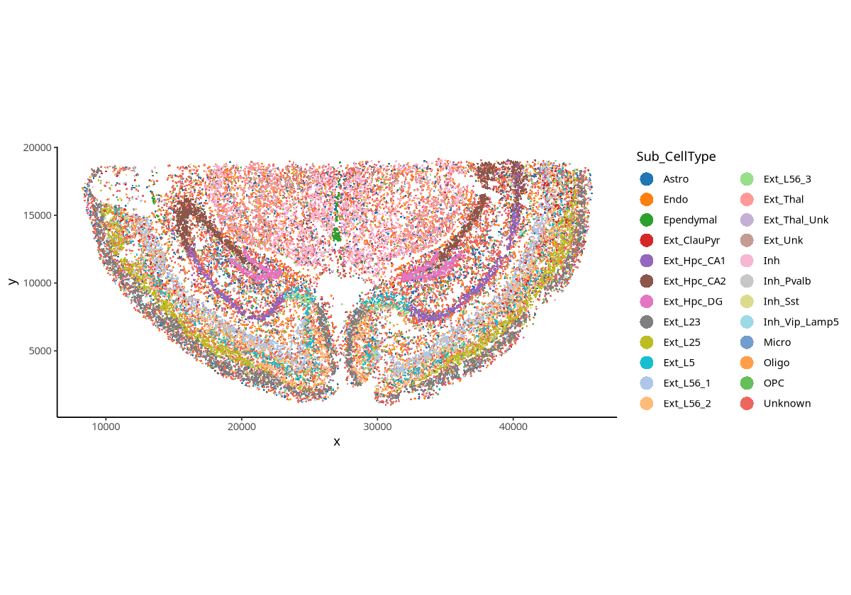
Grid-based Analysis
scider can perform grid-based density analysis on spatial transcriptomics data.
Density Calculation
Use the function gridDensity to calculate the density for each cell type. The calculated density and grid information are stored in the metadata of the SpatialExperiment object.
spe <- gridDensity(spe,id = "Sub_CellType")“data contain duplicated points”
Warning message:
“data contain duplicated points”
Warning message:
“data contain duplicated points”
Warning message:
“data contain duplicated points”
names(metadata(spe))- 'grid_density'
- 'grid_info'
Sys.setenv(PROJ_LIB = "/PROJ2/FLOAT/weichendan/software/micromamba/envs/TumorBoundary/share/proj")
plotDensity(spe, probs = 0)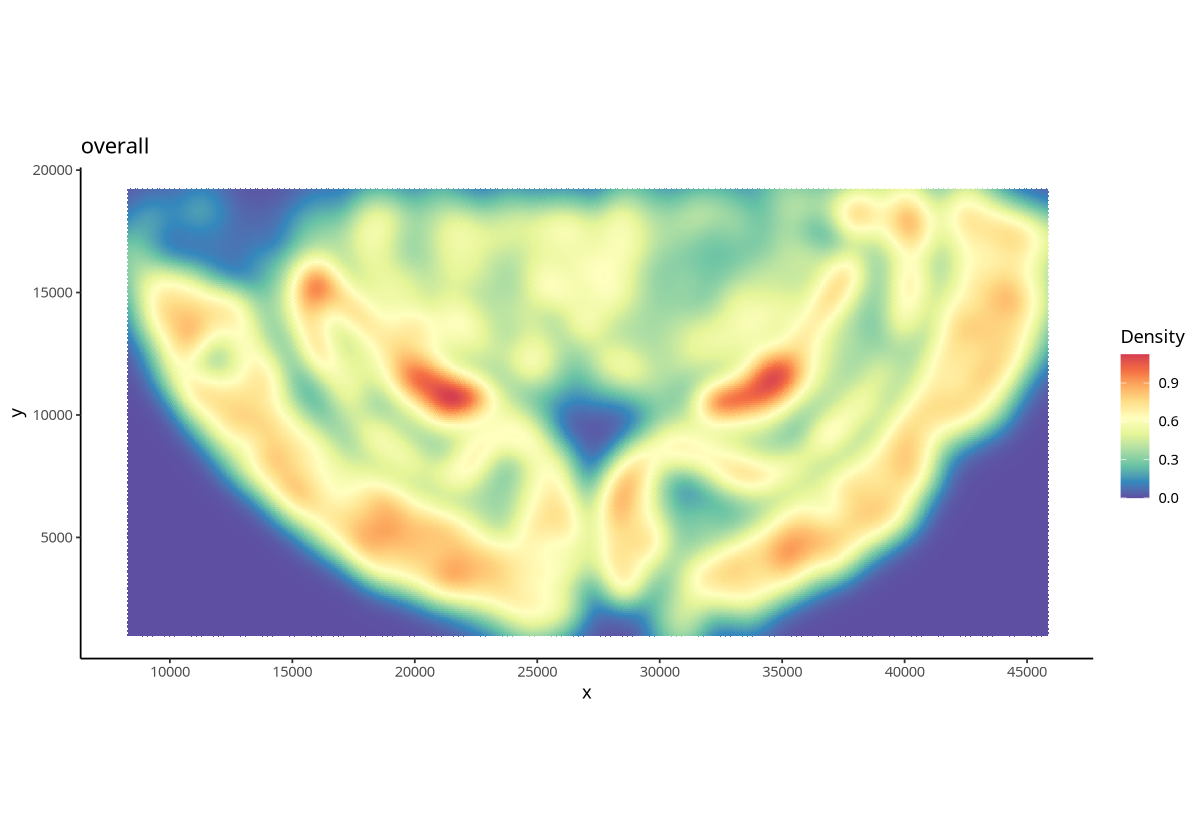
Figure Legend: Cell density of all cells across the entire tissue.
unique(colData(spe)$Sub_CellType)- 'Unknown'
- 'Endo'
- 'Ext_Thal_Unk'
- 'Inh'
- 'Astro'
- 'Ext_Hpc_DG'
- 'OPC'
- 'Ext_Hpc_CA2'
- 'Oligo'
- 'Micro'
- 'Inh_Pvalb'
- 'Ext_Hpc_CA1'
- 'Inh_Sst'
- 'Ependymal'
- 'Ext_L56_1'
- 'Ext_ClauPyr'
- 'Ext_Thal'
- 'Ext_L23'
- 'Inh_Vip_Lamp5'
- 'Ext_L25'
- 'Ext_L56_3'
- 'Ext_L56_2'
- 'Ext_L5'
- 'Ext_Unk'
plotDensity(spe, coi = "Ext_Hpc_DG",probs = 0)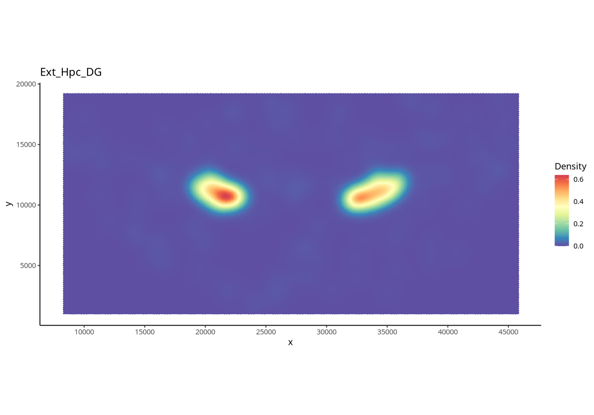
Figure Legend: Cell density of the specified cell type (Ext_Hpc_DG) across the entire tissue.
Automatic ROI Detection via Algorithm
After obtaining the grid-based density for each COI, we can detect Regions of Interest (ROI) based on density or user selection.
To automatically detect ROIs, we can use the function findROI. The detected ROIs are stored in the metadata of the SpatialExperiment object.
Here, we determine the ROI based on Ext_Hpc_DG cell density.
spe <- findROI(spe, coi = "Ext_Hpc_DG")spedim: 32285 32758
metadata(3): grid_density grid_info ext_hpc_dg_roi
assays(1): counts
rownames(32285): Xkr4 Gm1992 ... AC234645.1 AC149090.1
rowData names(0):
colnames(32758): AACAGGGTACTGAGGCTAAGGCACTAT
AAGCGAGTACATGCAGTGCTCTGCTTC ... TGCTTGCGCTGGCAGATCCTAATAACG
TCACAAGATGCGTATAAAGCGACGGAT
colData names(3): sample_id Sub_CellType Main_CellType
reducedDimNames(0):
mainExpName: NULL
altExpNames(0):
spatialCoords names(2) : x_centroid y_centroid
imgData names(1): sample_id
metadata(spe)$ext_hpc_dg_roicomponent members x y xcoord ycoord
factor character character character numeric numeric
1 1 227-190 227 190 30935 17377.9
2 1 228-190 228 190 31035 17377.9
3 1 229-190 229 190 31135 17377.9
4 1 227-191 227 191 30885 17464.5
5 1 228-191 228 191 30985 17464.5
... ... ... ... ... ... ...n 11879 21 261-122 261 122 34335 11488.9
11880 21 262-122 262 122 34435 11488.9
11881 21 263-122 263 122 34535 11488.9
11882 21 264-122 264 122 34635 11488.9
11883 21 265-122 265 122 34735 11488.9
plotROI(spe, roi = "Ext_Hpc_DG")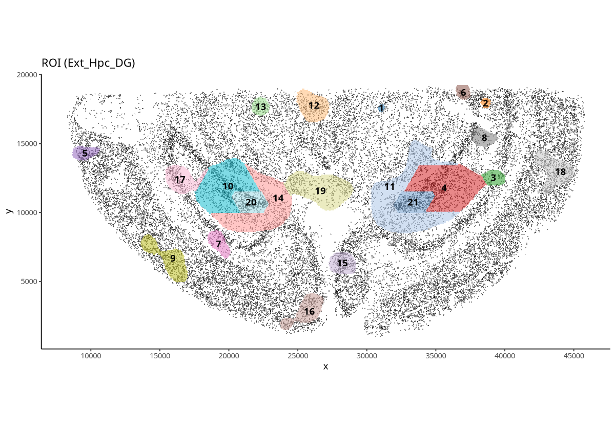
Figure Legend: Spatial display of ROIs for Ext_Hpc_DG cells. ROIs obtained focusing on the distribution density of Ext_Hpc_DG cells.
Density Correlation Between Cell Types
After defining Regions of Interest (ROIs), we can test the correlation between any two cell types within each ROI or globally, while using cubic spline functions or linear fitting to control for variation between ROIs.
plotDensCor(spe, celltype1 = "Ext_Hpc_CA2", celltype2 = "Ext_Hpc_DG", roi = "Ext_Hpc_DG")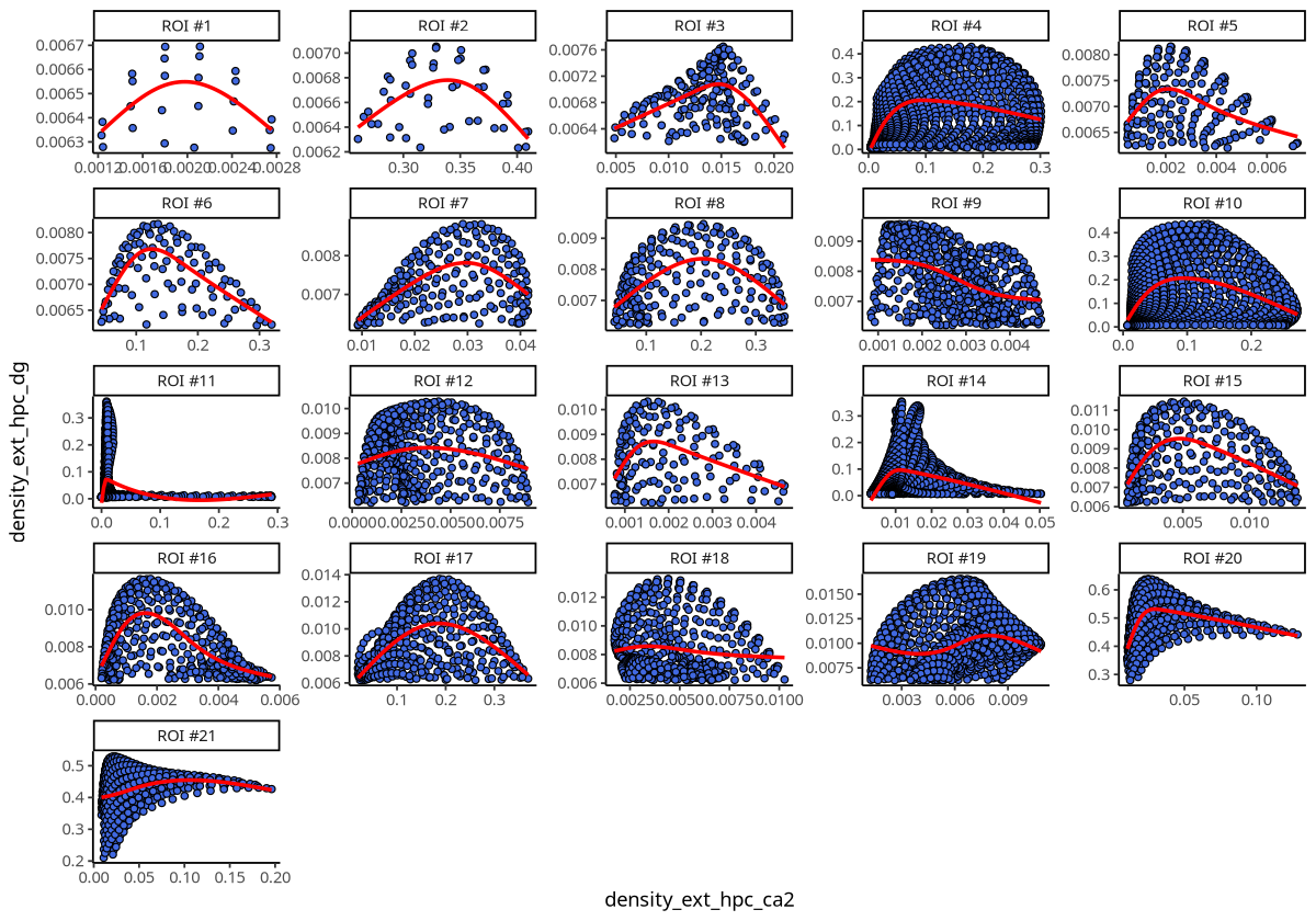
Figure Legend: Density correlation between Ext_Hpc_CA2 and Ext_Hpc_DG cell types in each ROI. Points represent grids of spatial transcriptomics data; x-axis is grid density of Ext_Hpc_CA2, y-axis is grid density of Ext_Hpc_DG.
plotDensCor(spe, celltype1 = "Ext_Hpc_CA2", celltype2 = "Ext_Hpc_DG")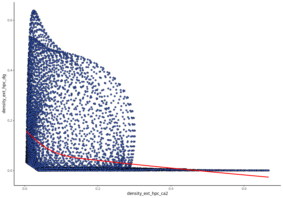
Figure Legend: Overall density correlation between Ext_Hpc_CA2 and Ext_Hpc_DG cell types. Points represent grids of spatial transcriptomics data; x-axis is grid density of Ext_Hpc_CA2, y-axis is grid density of Ext_Hpc_DG.
results <- corDensity(spe, roi = "Ext_Hpc_DG")Spatial correlation between each pair of cell types within each Ext_Hpc_DG Region of Interest (ROI):
head(as.data.frame(results$ROI))| celltype1 | celltype2 | ROI | ngrid | cor.coef | t | df | p.Pos | p.Neg | |
|---|---|---|---|---|---|---|---|---|---|
| <chr> | <chr> | <chr> | <dbl> | <dbl> | <dbl> | <dbl> | <dbl> | <dbl> | |
| 1 | Astro | Endo | 1 | 24 | 0.8530792 | 2.6455314 | 2.618330 | 0.044591309 | 0.9554087 |
| 2 | Astro | Endo | 2 | 46 | 0.9282104 | 4.9024113 | 3.861380 | 0.004391825 | 0.9956082 |
| 3 | Astro | Endo | 3 | 179 | -0.5480082 | -1.1226607 | 2.936478 | 0.827542915 | 0.1724571 |
| 4 | Astro | Endo | 4 | 1546 | -0.1131211 | -0.4393291 | 14.890164 | 0.666634098 | 0.3333659 |
| 5 | Astro | Endo | 5 | 179 | -0.7398525 | -2.1496765 | 3.821097 | 0.949385996 | 0.0506140 |
| 6 | Astro | Endo | 6 | 108 | 0.7589837 | 2.3418250 | 4.036009 | 0.039318671 | 0.9606813 |
Table Legend:
celltype1: Name of the first cell type, e.g., "Astro" (Astrocytes).
celltype2: Name of the second cell type, e.g., "Endo" (Endothelial cells).
ROI: Number of the Region of Interest (ROI), used to distinguish different spatial regions.
ngrid: Total number of grid points (or spatial units) in the ROI used to calculate spatial correlation, representing the number of location points involved in the calculation.
cor.coef: Spatial correlation coefficient between two cell types (celltype1 and celltype2) in the specified ROI, typically ranging from [-1, 1].
- Close to 1 indicates positive correlation (spatial distributions of the two cells tend to appear together)
- Close to -1 indicates negative correlation (spatial distributions of the two cells tend to repel each other)
- Close to 0 indicates no obvious spatial correlation
t: t-statistic used to test if the correlation is significant, calculated based on correlation test, used to measure the statistical significance of the correlation.
df: Degrees of freedom, related to the t-test, used to find the corresponding p-value, affected by sample size (ngrid).
p.Pos: p-value in a two-sided test where the correlation is positive (i.e., cor.coef > 0). It represents the probability of observing the current or stronger positive correlation under random conditions.
p.Neg: p-value in a two-sided test where the correlation is negative (i.e., cor.coef < 0). It represents the probability of observing the current or stronger negative correlation under random conditions.
Spatial correlation between each pair of cell types across all Ext_Hpc_DG Regions of Interest:
head(as.data.frame(results$overall))| celltype1 | celltype2 | cor.coef | p.Pos | p.Neg | |
|---|---|---|---|---|---|
| <chr> | <chr> | <dbl> | <dbl> | <dbl> | |
| 1 | Astro | Endo | 0.2267222225 | 0.006902633 | 0.54630570 |
| 2 | Astro | Ependymal | 0.0001576445 | 0.653084301 | 0.07044218 |
| 3 | Astro | Ext clau pyr | 0.0405023258 | 0.137978214 | 0.23472097 |
| 4 | Astro | Ext hpc ca1 | 0.0117007121 | 0.051401754 | 0.08106990 |
| 5 | Astro | Ext hpc ca2 | -0.1059310406 | 0.764804792 | 0.02204070 |
| 6 | Astro | Ext hpc dg | 0.1225401230 | 0.029504754 | 0.74864420 |
Table Legend:
celltype1: Name of the first cell type, e.g., "Astro" (Astrocytes).
celltype2: Name of the second cell type, e.g., "Endo" (Endothelial cells).
cor.coef: Spatial correlation coefficient between two cell types (celltype1 and celltype2) in the specified ROI, typically ranging from [-1, 1].
- Close to 1 indicates positive correlation (spatial distributions of the two cells tend to appear together)
- Close to -1 indicates negative correlation (spatial distributions of the two cells tend to repel each other)
- Close to 0 indicates no obvious spatial correlation
p.Pos: p-value in a two-sided test where the correlation is positive (i.e., cor.coef > 0). It represents the probability of observing the current or stronger positive correlation under random conditions.
p.Neg: p-value in a two-sided test where the correlation is negative (i.e., cor.coef < 0). It represents the probability of observing the current or stronger negative correlation under random conditions.
Spatial correlation between each pair of cell types on ROI regions:
options(repr.plot.height=7, repr.plot.width=10)
plotCorHeatmap(results$overall)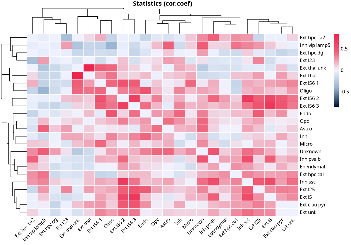
Figure Legend: Heatmap of spatial correlation between each pair of cell types on ROI regions. X-axis and Y-axis are cell types on ROI regions; color indicates the strength of spatial correlation.
Cell-based Analysis
Based on grid density, we can ask many biological questions about the data. For example, we might want to know if a cell type located in a high-density region of a specified cell type differs from the same cell type from a different density region of the specified cell.
Cell Annotation Based on Grid Density
To address this, we first need to divide cells into different grid density levels. This can be achieved using the contour recognition strategy of the getContour function.
spe <- getContour(spe, coi = "Ext_Hpc_DG", equal.cell = TRUE, id = "Sub_CellType")spedim: 32285 32758
metadata(4): grid_density grid_info ext_hpc_dg_roi ext_hpc_dg_contour
assays(1): counts
rownames(32285): Xkr4 Gm1992 ... AC234645.1 AC149090.1
rowData names(0):
colnames(32758): AACAGGGTACTGAGGCTAAGGCACTAT
AAGCGAGTACATGCAGTGCTCTGCTTC ... TGCTTGCGCTGGCAGATCCTAATAACG
TCACAAGATGCGTATAAAGCGACGGAT
colData names(5): sample_id Sub_CellType Main_CellType ext_hpc_dg_roi
ext_hpc_dg_contour
reducedDimNames(0):
mainExpName: NULL
altExpNames(0):
spatialCoords names(2) : x_centroid y_centroid
imgData names(1): sample_id
options(repr.plot.height=7, repr.plot.width=10)
plotContour(spe, coi = "Ext_Hpc_DG", id = "Sub_CellType")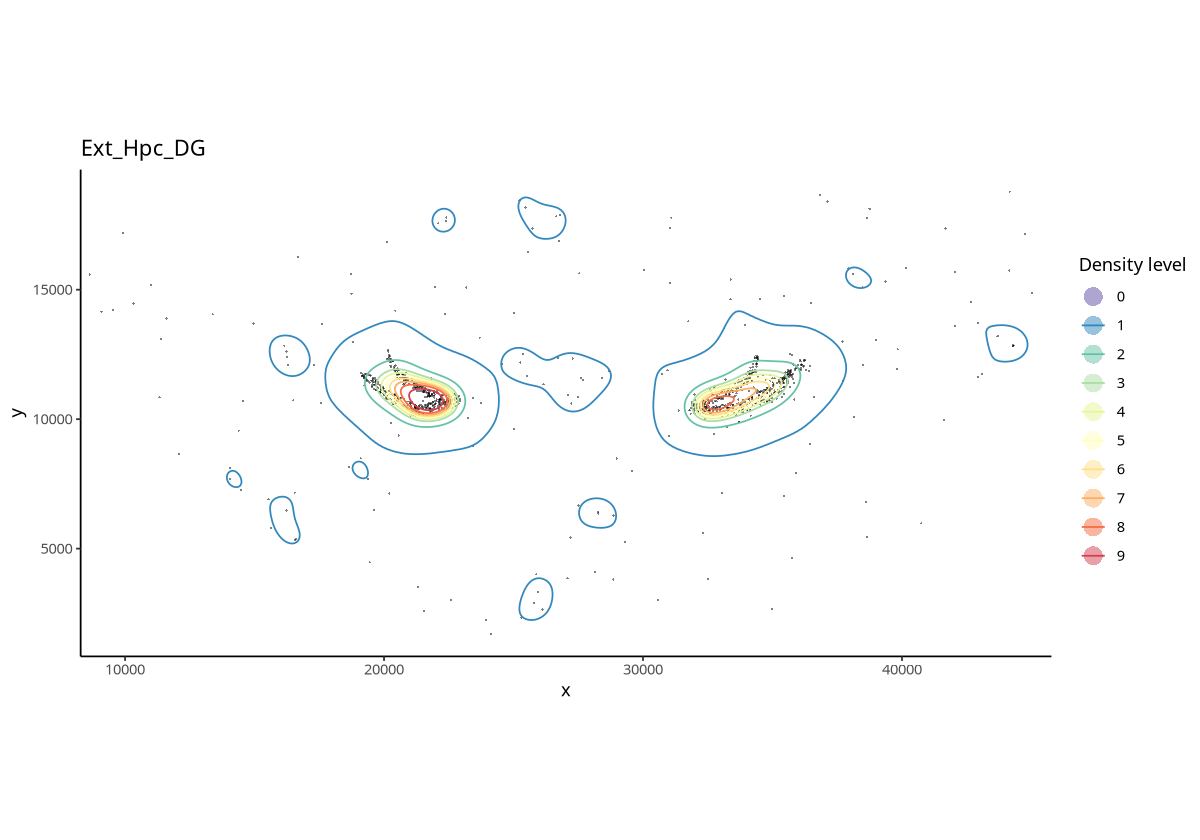
Figure Legend: Contour plot of Ext_Hpc_DG cells. Points represent cells; linear regions are different contour density regions.
Then, we can use the allocateCells function to cluster or annotate cells based on their location within each contour.
spe <- allocateCells(spe)Assigning cells to contour levels of Ext hpc dg
Linking to GEOS 3.12.2, GDAL 3.9.2, PROJ 9.5.0; sf_use_s2() is TRUE
spedim: 32285 32758
metadata(4): grid_density grid_info ext_hpc_dg_roi ext_hpc_dg_contour
assays(1): counts
rownames(32285): Xkr4 Gm1992 ... AC234645.1 AC149090.1
rowData names(0):
colnames(32758): AACAGGGTACTGAGGCTAAGGCACTAT
AAGCGAGTACATGCAGTGCTCTGCTTC ... TGCTTGCGCTGGCAGATCCTAATAACG
TCACAAGATGCGTATAAAGCGACGGAT
colData names(5): sample_id Sub_CellType Main_CellType ext_hpc_dg_roi
ext_hpc_dg_contour
reducedDimNames(0):
mainExpName: NULL
altExpNames(0):
spatialCoords names(2) : x_centroid y_centroid
imgData names(1): sample_id
plotSpatial(spe, group.by = "ext_hpc_dg_contour", pt.alpha = 0.5)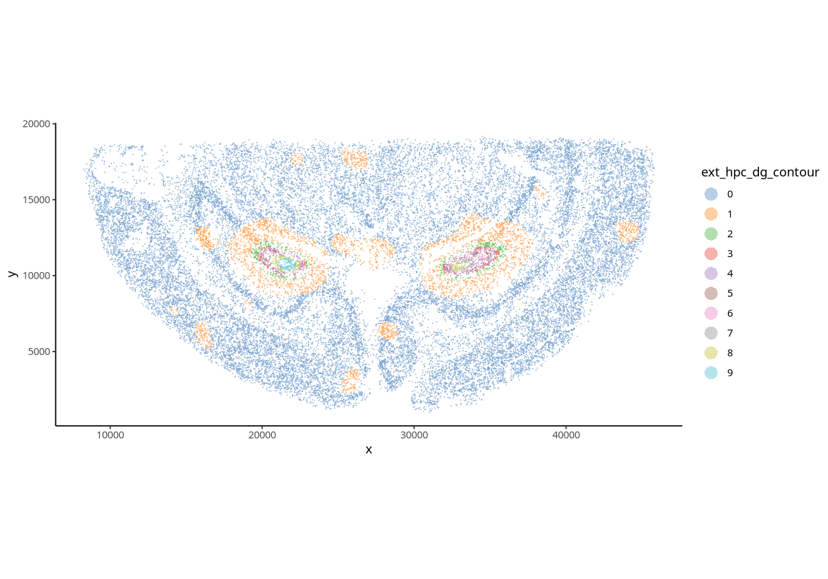
Figure Legend: Clustering obtained based on contour density regions of Ext_Hpc_DG cells. Points represent cells; different colors represent different clusters.
Visualization of Cell Type Composition for Each Level
plotCellCompo(spe, contour = "Ext_Hpc_DG", id = "Sub_CellType")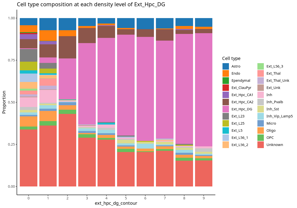
Figure Legend: Cell type proportion analysis for each contour region related to Ext_Hpc_DG cells. X-axis represents contour regions; Y-axis is cell type proportion.
plotCellCompo(spe, contour = "Ext_Hpc_DG", roi = "Ext_Hpc_DG", id = "Sub_CellType")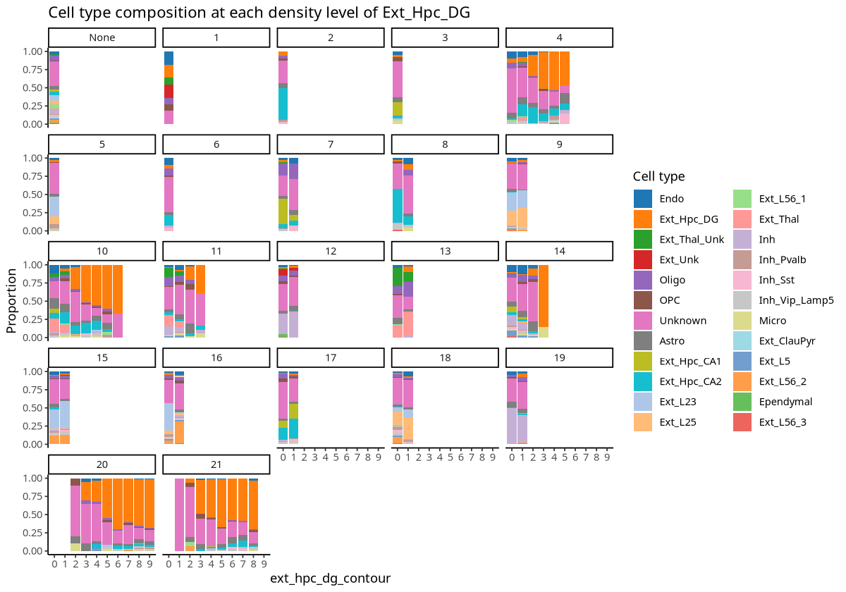
Figure Legend: Cell type proportion analysis for contour regions within each ROI region related to Ext_Hpc_DG cells. X-axis represents contour regions; Y-axis is cell type proportion; each small plot represents an ROI region.