scRNA-seq + scATAC-seq Multimodal Integration Tutorial (WNN / Label Transfer)

Author: SeekGene

Time: 19 min

Words: 3.7k words

Updated: 2026-02-28

Reads: 0 times

scATAC + RNA-seq Analysis Guide Notebooks Basic Analysis

# Load necessary R packages
suppressPackageStartupMessages({
  library(Seurat)
  library(Signac)
  library(EnsDb.Hsapiens.v86, lib.loc = "/PROJ2/FLOAT/shumeng/apps/miniconda3/envs/python3.10/lib/R/library")
  library(BSgenome.Hsapiens.UCSC.hg38,lib = "/PROJ2/FLOAT/shumeng/apps/miniconda3/envs/python3.10/lib/R/library")
  library(biovizBase, lib = "/PROJ2/FLOAT/shumeng/apps/miniconda3/envs/python3.10/lib/R/library")
  #library(BSgenome.Mmusculus.UCSC.mm10)
  #library(EnsDb.Mmusculus.v79)
  library(dplyr)
  library(ggplot2)
  library(patchwork)
})

# Set random seed
set.seed(1234)

# Set Seurat options (Note: 8000 * 1024^2 is actually 8GB)
options(future.globals.maxSize = 8000 * 1024^2)  # 8GB

my36colors <-c( '#E5D2DD', '#53A85F', '#F1BB72', '#F3B1A0', '#D6E7A3', '#57C3F3', '#476D87',
                '#E95C59', '#E59CC4', '#AB3282', '#23452F', '#BD956A', '#8C549C', '#585658',
                '#9FA3A8', '#E0D4CA', '#5F3D69', '#C5DEBA', '#58A4C3', '#E4C755', '#F7F398',
                '#AA9A59', '#E63863', '#E39A35', '#C1E6F3', '#6778AE', '#91D0BE', '#B53E2B',
                '#712820', '#DCC1DD', '#CCE0F5', '#CCC9E6', '#625D9E', '#68A180', '#3A6963',
                '#968175', "#6495ED", "#FFC1C1",'#f1ac9d','#f06966','#dee2d1','#6abe83','#39BAE8','#B9EDF8','#221a12',
                '#b8d00a','#74828F','#96C0CE','#E95D22','#017890')

Data Loading and Preparation

To get started, please prepare the following files:

scRNA-seq Data (Expression Matrix)
├── RNA_SAMple
│ ├── filtered_feature_bc_matrix
│ │ ├── barcodes.tsv.gz (Cell Barcodes)
│ │ ├── features.tsv.gz (Gene List)
│ │ └── matrix.mtx.gz (Sparse Expression Matrix)

scATAC-seq Data (Peaks Matrix + Fragments)
├── ATAC_SAMple
│ ├── filtered_peaks_bc_matrix
│ │ ├── barcodes.tsv.gz (Cell Barcodes)
│ │ ├── features.tsv.gz (Peaks List)
│ │ └── matrix.mtx.gz (Sparse Count Matrix)
│ ├── ATAC_SAMple_fragments.tsv.gz (Genomic coordinates for each sequencing read, for QC like TSS enrichment/nucleosome signal)
│ ├── ATAC_SAMple_fragments.tsv.gz.tbi (Index file for fragments)
│ └── per_barcode_metrics.csv (Optional per-cell QC metrics)

Tips:

• If using data generated by different platforms/pipelines, ensure they can be read as equivalent sparse matrix and fragment files.
• Try to ensure RNA and ATAC come from similar samples/conditions for more reliable label transfer.

Get Gene Annotation Information

We will retrieve human genome annotations (gene positions, transcripts, exons, TSS, etc.) from the EnsDb database. This information is used for:

• Calculating ATAC TSS enrichment (determining if open chromatin is more concentrated near transcription start sites)
• Constructing "Gene Activity Matrix" (mapping peaks signals to genes)

Please ensure:

• Species matches reference genome version (e.g., EnsDb.Hsapiens.v86 corresponds to hg38)
• Chromosome naming style is consistent (e.g., all use prefixes like chr1, chr2)

# Get gene annotation information (suppress warnings and messages)
suppressWarnings({
  suppressMessages({
    annotation <- GetGRangesFromEnsDb(ensdb = EnsDb.Hsapiens.v86)
    seqlevels(annotation) <- paste0('chr', seqlevels(annotation))
    genome(annotation) <- 'hg38'
  })
})

# Set parallel computing (suppress output, optional)
suppressPackageStartupMessages({
  library(future)
})
plan("multicore", workers = 4)

Load scRNA-seq Data

We will read the expression matrix (triplet of barcodes/features/matrix) and create a standard Seurat object:

• counts: Gene counts per cell
• meta.data: Will include sample info, QC metrics, clusters/cell types, etc., later

The resulting object will serve as the "reference" for transferring labels to ATAC cells.

options(warn = -1)
# Define scRNA-seq data path
rna_sample_name <- 'joint34'
rna_counts_path <- file.path(rna_sample_name, 'filtered_feature_bc_matrix')

# Read scRNA-seq data
rna_counts <- Read10X(rna_counts_path)

# Create scRNA-seq Seurat object
rna_obj <- CreateSeuratObject(
  counts = rna_counts,
  project = "RNA_sample",
  min.cells = 3,
  min.features = 200
)

# Add sample ID
rna_obj$orig.ident <- 'joint34'
rna_obj$Sample <- 'joint34'
rna_obj$technology <- 'RNA'
options(warn = 0)
# scRNA-seq data loading complete

Load scATAC-seq Data

Here we will read:

• filtered_peaks_bc_matrix: Sparse count matrix of peaks × cells (representing open chromatin counts)
• fragments.tsv.gz: Genomic coordinates of each read (used for QC such as TSS enrichment, nucleosome signal)

Then create ChromatinAssay using Signac and wrap it as a Seurat object. This object will serve as the 'query' to receive label transfer from RNA.

# Define scATAC-seq data path
atac_sample_name <- 'joint41'
atac_counts_path <- file.path(atac_sample_name, 'filtered_peaks_bc_matrix')
atac_fragments_path <- file.path(atac_sample_name, paste0(atac_sample_name, '_A_fragments.tsv.gz'))
#atac_metadata_path <- file.path(atac_sample_name, 'per_barcode_metrics.csv')

# Read scATAC-seq data
atac_counts <- Read10X(atac_counts_path)

# Read QC metrics metadata
#atac_metadata <- read.csv(
#  file = atac_metadata_path,
#  header = TRUE,
#  row.names = 1
#)

# Create ChromatinAssay object
chrom_assay <- CreateChromatinAssay(
  counts = atac_counts,
  sep = c(':', '-'),
  fragments = atac_fragments_path,
  annotation = annotation,
  min.cells = 3,
  min.features = 200
)

# Create scATAC-seq Seurat object
atac_obj <- CreateSeuratObject(
  counts = chrom_assay,
  assay = "ATAC",
  project = "ATAC_sample"#,meta.data = atac_metadata
)

# Add sample ID
atac_obj$orig.ident <- 'joint41'
atac_obj$Sample <- 'joint41'
atac_obj$technology <- 'joint41'

# scATAC-seq data reading completed

output

Computing hash

Warning message:
"Keys should be one or more alphanumeric characters followed by an underscore, setting key from atac to atac_"

Data Preprocessing

Before integration, both types of data need to be 'cleaned' separately:

• QC (Quality Control): Remove low-quality cells (e.g., high mitochondrial ratio, low ATAC TSS enrichment)
• Preliminary Normalization/Dimensionality Reduction: Prepare for finding anchors and visualization

Thresholds vary by dataset; common metrics and visualization methods are provided below to help adjust thresholds based on distribution.

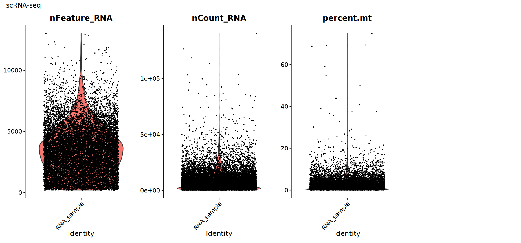
scRNA-seq Data Quality Control

Common QC metrics:

• percent.mt: Mitochondrial gene proportion. High values usually indicate cell damage or RNA leakage.
• nFeature_RNA: Number of detected genes. Low values may indicate empty droplets; high values may indicate doublets/multiplets.
• nCount_RNA: Total counts. Correlated with sequencing depth; requires distribution check to identify outliers.

There are no 'one-size-fits-all' thresholds; empirical filtering should be based on data distribution (violin plots/scatter plots).

# Calculate mitochondrial gene expression proportion
suppressWarnings({
    rna_obj[["percent.mt"]] <- PercentageFeatureSet(rna_obj, pattern = "^MT-")
})

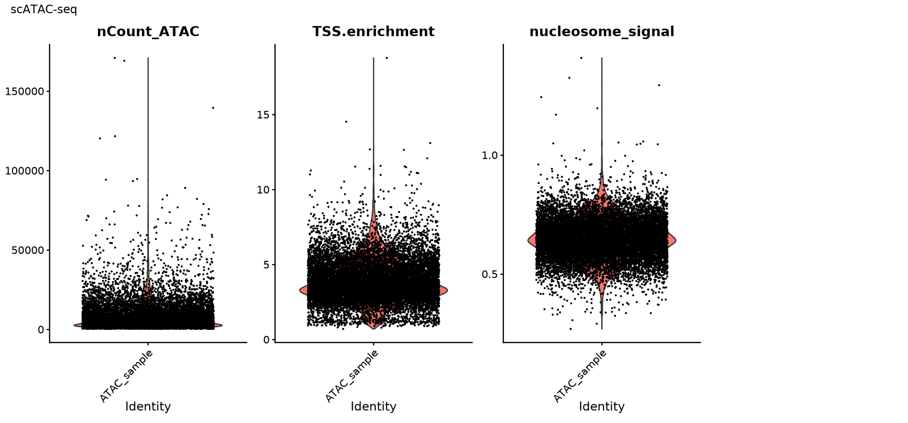
scATAC-seq Data Quality Control

Common QC metrics:

• TSS.enrichment (TSS enrichment score): Higher is better, indicating signal concentration near transcription start sites; low values may indicate high background or poor cell viability.
• nucleosome_signal (Nucleosome signal): Reflects nucleosome periodicity signal; typically lower is better.
• nCount_ATAC: Total ATAC counts; extremely low or high values require caution.

Actual thresholds should be set based on data distribution and judged in conjunction with fragment quality, doublet rates, etc.

# Set default assay to peaks
DefaultAssay(atac_obj) <- 'ATAC'

# Calculate TSS enrichment score
atac_obj <- TSSEnrichment(atac_obj)

# Calculate nucleosome signal
atac_obj <- NucleosomeSignal(atac_obj)

output

Extracting TSS positions

Extracting fragments at TSSs


Computing TSS enrichment score

Quality Control Visualization

Use violin plots to view the distribution/outliers of QC metrics to help select thresholds:

• RNA：nFeature_RNA、nCount_RNA、percent.mt
• ATAC：nCount_ATAC、TSS.enrichment、nucleosome_signal

Suggestions:

• Observe if there are obvious long tails or bimodal distributions
• Try multiple thresholds and compare if downstream clustering/UMAP is clearer

# Visualize scRNA-seq QC metrics
suppressWarnings({
    options(repr.plot.width = 15, repr.plot.height = 7)
    p1 <- VlnPlot(rna_obj, 
              features = c("nFeature_RNA", "nCount_RNA", "percent.mt"),
              ncol = 4, pt.size = 0.1) +
      plot_annotation(title = "scRNA-seq")

    print(p1)

    # Visualize scATAC-seq QC metrics
    p2 <- VlnPlot(atac_obj, 
              features = c("nCount_ATAC", "TSS.enrichment", "nucleosome_signal"),
              ncol = 4, pt.size = 0.1) +
      plot_annotation(title = "scATAC-seq")

    print(p2)
})

Quality Control Filtering

Select thresholds based on the previous distribution and filter low-quality cells. Tips:

• A decrease in cell number after filtering is normal; the key is to improve the signal-to-noise ratio
• Please record the thresholds used and the reasons for reproducibility and team communication

# Filter scRNA-seq data
cat('scRNA-seq cell count before filtering:', ncol(rna_obj), '\n')
rna_obj <- subset(rna_obj, 
                  subset = nFeature_RNA > 200 & 
                          nFeature_RNA < 10000 & 
                          percent.mt < 20)
cat('scRNA-seq cell count after filtering:', ncol(rna_obj), '\n')
# Filter scATAC-seq data
cat('scATAC-seq cell count before filtering:', ncol(atac_obj), '\n')
atac_obj <- subset(atac_obj,
                   subset = nCount_ATAC > 500 &
                           nCount_ATAC < 50000 &
                           TSS.enrichment > 1 &
                           nucleosome_signal < 1)
cat('scATAC-seq cell count after filtering:', ncol(atac_obj), '\n')

output

过滤前scRNA-seq细胞数： 13104
过滤后scRNA-seq细胞数： 13013
过滤前scATAC-seq细胞数： 13109
过滤后scATAC-seq细胞数： 12931

Data Normalization

We will perform adapted normalization/dimensionality reduction for both data types:

• RNA: Normalize → Select variable genes → Scale → PCA/UMAP → Neighbor graph and clustering
• ATAC: TF-IDF → Select important features (peaks) → LSI (similar to PCA) → UMAP

Objective: To bring samples with different sequencing depths and count scales into a comparable space and preliminarily reveal the principal structure, facilitating subsequent search for 'cross-modal anchors'.

# scRNA-seq data normalization
suppressWarnings({
  suppressMessages({
      rna_obj <- NormalizeData(rna_obj)
      rna_obj <- FindVariableFeatures(rna_obj,nfeatures=4000)
      rna_obj <- ScaleData(rna_obj)
      rna_obj <- RunPCA(rna_obj)
      rna_obj <- RunUMAP(rna_obj, dims = 1:30)
      rna_obj <- FindNeighbors(rna_obj, dims = 1:30)
      rna_obj <- FindClusters(rna_obj, resolution = 0.5)
  })
})

output

Modularity Optimizer version 1.3.0 by Ludo Waltman and Nees Jan van Eck

Number of nodes: 13013
Number of edges: 445565

Running Louvain algorithm...n Maximum modularity in 10 random starts: 0.9026
Number of communities: 15
Elapsed time: 1 seconds

# scATAC-seq data normalization
suppressWarnings({
  suppressMessages({
      atac_obj <- RunTFIDF(atac_obj)
      atac_obj <- FindTopFeatures(atac_obj, min.cutoff = "q0")
      atac_obj <- RunSVD(atac_obj)
      atac_obj <- RunUMAP(atac_obj, reduction = "lsi", dims = 2:30, reduction.name = "umap.atac", reduction.key = "atacUMAP_")
        })
})

Gene Activity Score Calculation

To connect ATAC 'openness' with RNA 'expression levels', we need to map peak signals to genes to obtain 'gene activity scores'. It is not direct expression, but statistically approximates the potential expression activity of a gene, serving as a key bridge for cross-modal integration.

Calculate Gene Activity Matrix

Idea: Count peaks signals associated with each gene (e.g., gene body + upstream/downstream promoter regions) to accumulate an "activity score" for that gene in each cell.

• Typical approach takes a window of ~2kb upstream and ~1kb downstream of TSS (adjustable as needed)
• The resulting ACTIVITY assay will be used to establish anchors with the RNA RNA assay

# Calculate Gene Activity Score
# Calculate activity score using gene body and promoter regions
suppressWarnings({
    DefaultAssay(atac_obj)="ATAC"
    gene.activities <- GeneActivity(
        object = atac_obj,
        features = VariableFeatures(rna_obj),extend.upstream = 2000,extend.downstream = 1000)

    # Add gene activity matrix as a new assay
    atac_obj[['ACTIVITY']] <-  CreateAssayObject(counts = gene.activities)
    DefaultAssay(atac_obj) <- "ACTIVITY"
    # Normalize gene activity data
    atac_obj <- NormalizeData(atac_obj)
    atac_obj <- ScaleData(atac_obj, features = rownames(atac_obj))
})

output

Extracting gene coordinates

Extracting reads overlapping genomic regions

Centering and scaling data matrix

Multimodal Data Integration

Now we match across modalities using "RNA Expression Matrix (Reference)" and "ATAC Gene Activity Matrix (Query)". Core tasks:

• Find cross-modal "correspondences" (anchors)
• Transfer labels from "Reference" to "Query" cells

Find Integration Anchors

"Anchors" are key to aligning two data spaces. The method uses CCA/LSI to find a set of highly comparable feature subspaces between RNA and ATAC (gene activity), establishing a mutually projectable coordinate system.

# Set default assay of scATAC-seq object to ACTIVITY (Gene Activity Score)
DefaultAssay(atac_obj) <- 'ACTIVITY'
suppressWarnings({
  suppressMessages({
      # Find integration anchors
      transfer.anchors <- FindTransferAnchors(
          reference = rna_obj,
          query = atac_obj,
          features = VariableFeatures(object = rna_obj),
          reference.assay = 'RNA',
          query.assay = 'ACTIVITY',
          k.anchor = 30,
          k.filter = 50 ,
          reduction = 'cca'
      )
  })
})

Predict Cell Type Labels

Once anchors are established, "Reference" labels (like cell_type or Seurat_clusters) can be transferred to ATAC cells:

• Output predicted.id is the predicted type/cluster for each ATAC cell
• Prediction scores are also obtained to measure confidence (this tutorial shows cluster labels)

Suggestions:

• Use UMAP to check if predicted distribution matches RNA structure
• Perform sanity check using marker genes/known biological knowledge

# Predict cluster labels for scATAC-seq cells
predicted.labels <- TransferData(
  anchorset = transfer.anchors,
  refdata = rna_obj$seurat_clusters, # Actual cell annotation from scRNA-seq data, choose according to actual scRNA-seq annotation

  weight.reduction = atac_obj[['lsi']],
  dims = 2:30
)

# Add predicted labels to scATAC-seq object
atac_obj <- AddMetaData(atac_obj, metadata = predicted.labels)

output

Finding integration vectors

Finding integration vector weights

Predicting cell labels

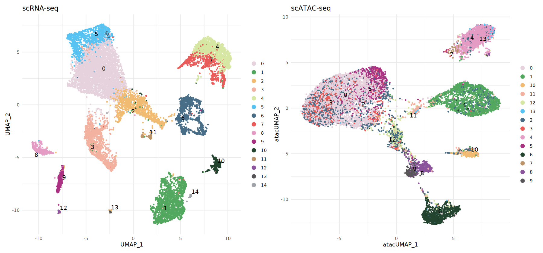
Visualize scATAC-seq Cell Types

Here we display side-by-side:

• RNA: Clustering from reference data/calculated
• ATAC: predicted.id obtained via label transfer

Colors correspond to the same categories, facilitating direct comparison of structural consistency.

# scRNA-seq Data Visualization
options(repr.plot.width = 15, repr.plot.height = 7)
p1 <- DimPlot(rna_obj, 
              group.by = 'seurat_clusters', 
              label = TRUE, 
              repel = TRUE,
              pt.size = 0.5) + 
      ggtitle('scRNA-seq') +
      theme_minimal() +
      scale_color_manual(values = my36colors)

# scATAC-seq Data Visualization (Based on Predicted Labels)

p2 <- DimPlot(atac_obj, 
              group.by = 'predicted.id', 
              label = TRUE, 
              repel = TRUE,
              pt.size = 0.5) + 
      ggtitle('scATAC-seq') +
      theme_minimal() +
      scale_color_manual(values = my36colors)
p1 | p2
pdf("scRNA_scATAC_UMAP.pdf", width = 10, height = 5)
print(p1 | p2)
dev.off()

pdf: 2

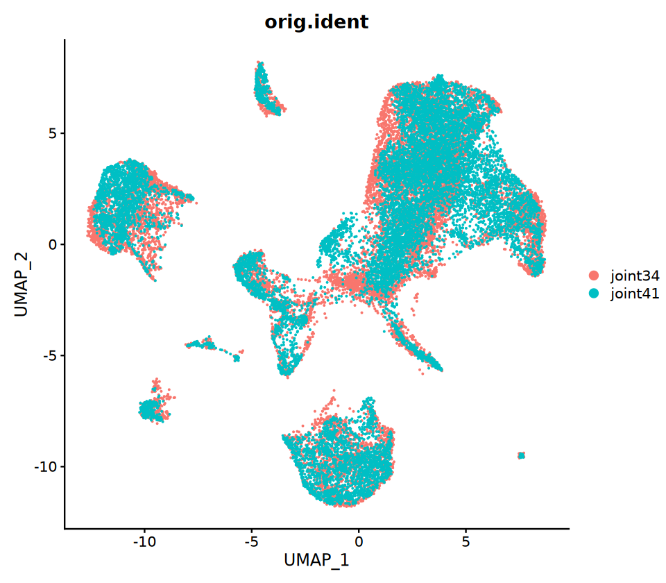
Co-embedding Analysis (Optional)

Purpose: Place RNA and ATAC cells on the same UMAP to observe cross-modal consistency. Method Highlights:

• First use anchors to "impute/project" RNA expression matrix onto ATAC to get "imputed expression matrix" for ATAC cells
• Merge both and then perform unified dimensionality reduction and UMAP

Note: Co-embedding is mainly a visualization tool, not equivalent to real same-cell multi-omics observations. Please interpret with biological common sense.

# Calculate Co-embedding
suppressWarnings({
  suppressMessages({
      genes.use <- VariableFeatures(rna_obj)
      refdata <- GetAssayData(rna_obj, assay = "RNA", slot = "data")[genes.use, ]

# refdata (input) contains a scRNA-seq expression matrix for the scRNA-seq cells.  imputation
# (output) will contain an imputed scRNA-seq matrix for each of the ATAC cells
     imputation <- TransferData(anchorset = transfer.anchors, refdata = refdata, weight.reduction = "cca",dims=1:30)
     atac_obj[["RNA"]] <- imputation
     coembed <- merge(x = rna_obj, y = atac_obj)

     coembed <- ScaleData(coembed, features = genes.use, do.scale = FALSE)
     coembed <- RunPCA(coembed, features = genes.use, verbose = FALSE)
     coembed <- RunUMAP(coembed, dims = 1:30)
  })
})
options(repr.plot.width = 8, repr.plot.height = 7)
p3=DimPlot(coembed, group.by = c("orig.ident"))
p3
pdf("coembed_UMAP.pdf", width = 10, height = 5)
print(p3)
dev.off()

pdf: 2

Results Summary and Saving

After completion, please save key objects for reproduction and subsequent analysis:

• scRNA_processed.rds: Normalized/reduced/clustered RNA object
• scATAC_processed.rds: QC/normalized/predicted-label ATAC object (includes ACTIVITY)
• coembed.rds: Co-embedding object (if step executed)
• session_info.txt: Session info for reproduction

# Save analysis objects
saveRDS(rna_obj, file = "./scRNA_processed.rds")
saveRDS(atac_obj, file = "./scATAC_processed.rds")
saveRDS(coembed, file = "./coembed.rds")

Advanced Analysis Suggestions

After completing basic integration, you can go further:

Transcription Factor Motif Analysis

• Use FindMotifs() to find enriched TF motifs in Differentially Accessible Regions (DARs)
• Infer TF activity changes combining RNA expression or gene activity

Gene Regulatory Network (GRN) and Peaks-to-Gene Links

• Use LinkPeaks() to identify potential regulatory relationships between peaks and target genes
• If only single-omics data is available, consider imputation or pseudo-bulk to establish expression-accessibility correspondence; best practice is direct validation with single-cell multi-omics data

Developmental Trajectory/Pseudotime Analysis

• Perform cell trajectory inference in integration space
• Compare dynamic changes in gene expression and accessibility along the trajectory

Differential Accessibility and Differential Expression

• Compare differential peaks and differential genes between different cell types/states
• Identify cell type-specific regulatory elements

Functional Enrichment

• Perform GO/KEGG enrichment on differential genes or genes associated with differential peaks
• Interpret cell functional characteristics combining known pathways

sessionInfo()

output

R version 4.3.3 (2024-02-29)
Platform: x86_64-conda-linux-gnu (64-bit)
Running under: Debian GNU/Linux 12 (bookworm)

Matrix products: default
BLAS/LAPACK: /jp_envs/envs/common/lib/libopenblasp-r0.3.29.so; LAPACK version 3.12.0

locale:
[1] LC_CTYPE=C.UTF-8 LC_NUMERIC=C LC_TIME=C.UTF-8
[4] LC_COLLATE=C.UTF-8 LC_MONETARY=C.UTF-8 LC_MESSAGES=C.UTF-8
[7] LC_PAPER=C.UTF-8 LC_NAME=C LC_ADDRESS=C
[10] LC_TELEPHONE=C LC_MEASUREMENT=C.UTF-8 LC_IDENTIFICATION=C

time zone: Asia/Shanghai
tzcode source: system (glibc)

attached base packages:
[1] stats4 stats graphics grDevices utils datasets methods
[8] base

other attached packages:
[1] future_1.40.0 repr_1.1.7
[3] patchwork_1.3.0 ggplot2_3.5.2
[5] dplyr_1.1.4 biovizBase_1.50.0
[7] BSgenome.Hsapiens.UCSC.hg38_1.4.5 BSgenome_1.70.1
[9] rtracklayer_1.62.0 BiocIO_1.12.0
[11] Biostrings_2.70.1 XVector_0.42.0
[13] EnsDb.Hsapiens.v86_2.99.0 ensembldb_2.26.0
[15] AnnotationFilter_1.26.0 GenomicFeatures_1.54.1
[17] AnnotationDbi_1.64.1 Biobase_2.62.0
[19] GenomicRanges_1.54.1 GenomeInfoDb_1.38.1
[21] IRanges_2.36.0 S4Vectors_0.40.2
[23] BiocGenerics_0.48.1 Signac_1.10.0
[25] SeuratObject_4.1.4 Seurat_4.4.0

loaded via a namespace (and not attached):
[1] ProtGenerics_1.34.0 matrixStats_1.5.0
[3] spatstat.sparse_3.1-0 bitops_1.0-9
[5] httr_1.4.7 RColorBrewer_1.1-3
[7] tools_4.3.3 sctransform_0.4.1
[9] backports_1.5.0 R6_2.6.1
[11] lazyeval_0.2.2 uwot_0.2.3
[13] withr_3.0.2 sp_2.2-0
[15] prettyunits_1.2.0 gridExtra_2.3
[17] progressr_0.15.1 cli_3.6.4
[19] Cairo_1.6-2 spatstat.explore_3.4-2
[21] labeling_0.4.3 spatstat.data_3.1-6
[23] ggridges_0.5.6 pbapply_1.7-2
[25] Rsamtools_2.18.0 pbdZMQ_0.3-13
[27] foreign_0.8-87 R.utils_2.13.0
[29] dichromat_2.0-0.1 parallelly_1.43.0
[31] rstudioapi_0.15.0 RSQLite_2.3.9
[33] generics_0.1.3 ica_1.0-3
[35] spatstat.random_3.3-3 Matrix_1.6-5
[37] ggbeeswarm_0.7.2 abind_1.4-5
[39] R.methodsS3_1.8.2 lifecycle_1.0.4
[41] yaml_2.3.10 SummarizedExperiment_1.32.0
[43] SparseArray_1.2.2 BiocFileCache_2.10.1
[45] Rtsne_0.17 grid_4.3.3
[47] blob_1.2.4 promises_1.3.2
[49] crayon_1.5.3 miniUI_0.1.1.1
[51] lattice_0.22-7 cowplot_1.1.3
[53] KEGGREST_1.42.0 pillar_1.10.2
[55] knitr_1.49 rjson_0.2.23
[57] future.apply_1.11.3 codetools_0.2-20
[59] fastmatch_1.1-6 leiden_0.4.3.1
[61] glue_1.8.0 spatstat.univar_3.1-2
[63] data.table_1.17.0 vctrs_0.6.5
[65] png_0.1-8 gtable_0.3.6
[67] cachem_1.1.0 xfun_0.50
[69] S4Arrays_1.2.0 mime_0.13
[71] survival_3.8-3 RcppRoll_0.3.1
[73] fitdistrplus_1.2-2 ROCR_1.0-11
[75] nlme_3.1-168 bit64_4.5.2
[77] progress_1.2.3 filelock_1.0.3
[79] RcppAnnoy_0.0.22 irlba_2.3.5.1
[81] vipor_0.4.7 KernSmooth_2.23-26
[83] rpart_4.1.23 colorspace_2.1-1
[85] DBI_1.2.3 Hmisc_5.2-1
[87] nnet_7.3-19 ggrastr_1.0.2
[89] tidyselect_1.2.1 bit_4.5.0.1
[91] compiler_4.3.3 curl_6.0.1
[93] htmlTable_2.4.3 xml2_1.3.6
[95] DelayedArray_0.28.0 plotly_4.10.4
[97] checkmate_2.3.2 scales_1.3.0
[99] lmtest_0.9-40 rappdirs_0.3.3
[101] stringr_1.5.1 digest_0.6.37
[103] goftest_1.2-3 spatstat.utils_3.1-3
[105] rmarkdown_2.29 htmltools_0.5.8.1
[107] pkgconfig_2.0.3 base64enc_0.1-3
[109] MatrixGenerics_1.14.0 dbplyr_2.5.0
[111] fastmap_1.2.0 rlang_1.1.5
[113] htmlwidgets_1.6.4 shiny_1.10.0
[115] farver_2.1.2 zoo_1.8-14
[117] jsonlite_2.0.0 BiocParallel_1.36.0
[119] R.oo_1.27.0 VariantAnnotation_1.48.1
[121] RCurl_1.98-1.16 magrittr_2.0.3
[123] Formula_1.2-5 GenomeInfoDbData_1.2.11
[125] IRkernel_1.3.2 munsell_0.5.1
[127] Rcpp_1.0.14 reticulate_1.42.0
[129] stringi_1.8.7 zlibbioc_1.48.0
[131] MASS_7.3-60.0.1 plyr_1.8.9
[133] parallel_4.3.3 listenv_0.9.1
[135] ggrepel_0.9.6 deldir_2.0-4
[137] IRdisplay_1.1 splines_4.3.3
[139] tensor_1.5 hms_1.1.3
[141] igraph_2.0.3 uuid_1.2-1
[143] spatstat.geom_3.3-6 reshape2_1.4.4
[145] biomaRt_2.58.0 XML_3.99-0.17
[147] evaluate_1.0.3 httpuv_1.6.15
[149] RANN_2.6.2 tidyr_1.3.1
[151] purrr_1.0.4 polyclip_1.10-7
[153] scattermore_1.2 xtable_1.8-4
[155] restfulr_0.0.15 later_1.4.2
[157] viridisLite_0.4.2 tibble_3.2.1
[159] memoise_2.0.1 beeswarm_0.4.0
[161] GenomicAlignments_1.38.0 cluster_2.1.8.1
[163] globals_0.16.3