Single-cell Spatial Neighborhood Statistics: Spatial Distribution and Neighborhood Analysis

Author: SeekGene

Time: 12 min

Words: 2.4k words

Updated: 2026-02-28

Reads: 0 times

Spatial-seq Notebooks Niche Analysis

Load Analysis R Packages

library(Seurat)
library(qs)
library(dplyr)
library(tibble)
library(stringr)
library(ggplot2)
library(phenoptr)

output

Attaching SeuratObject

qs 0.27.3. Announcement: https://github.com/qsbase/qs/issues/103

Warning message:
“package ‘dplyr’ was built under R version 4.3.3”

Attaching package: ‘dplyr’

The following objects are masked from ‘package:stats’:

filter, lag

The following objects are masked from ‘package:base’:

intersect, setdiff, setequal, union

Warning message:
“package ‘tibble’ was built under R version 4.3.3”
Warning message:
“package ‘stringr’ was built under R version 4.3.3”
Warning message:
“package ‘ggplot2’ was built under R version 4.3.3”

Input Object Details

col_SAM: Sample column name in metadata
SAMple_name: Sample name to analyze
col_celltype: Cell type column name in metadata
analysis_celltype: Cell type to analyze

col_sam = "Sample"
sample_name = "T1"
col_celltype = "large_celltype"
analysis_celltype = "Neutrophils"

Read RDS and Metadata, Preprocess Data

data = readRDS("../../data/AY1739779861133/input.rds")

meta = read.delim("../../data/AY1739779861133/meta.tsv")
rownames(meta) = meta$barcode
data@meta.data = meta

Extract spatial sample info to analyze from RDS
Convert SeekSpace spatial coordinates: Pixel -> Actual (Conversion factor 0.2653)
Extract cell types to analyze
Calculate distances between each cell point

sub = subset(data,cells = rownames(data@meta.data[data@meta.data[[col_sam]] %in% sample_name,]))
sub@meta.data$barcode = rownames(sub@meta.data)
df_labels = sub@meta.data[,c("barcode",col_celltype)]
sub_position = Embeddings(sub,"spatial")
sub_position = sub_position*0.2653
sub_position = as.data.frame(sub_position)

Neu_barcode = rownames(sub@meta.data[sub@meta.data[[col_celltype]] %in% analysis_celltype,])
dist_matrix <- as.matrix(dist(sub_position, method = "euclidean"))

Calculate Spatial Neighborhood Composition in 4 Ranges

neigh_freq1 = data.frame()
for(threshold in c(20,50,100,200)){

    # Find neighbors for each point (excluding self)
    neighbors = apply(dist_matrix, 1, function(row) {
      nearby = which(row <= threshold & row > 0)  # row > 0 excludes self
      if (length(nearby) > 0) {
        paste(names(nearby), collapse = ";")  # Semicolon separated neighbors
      } else {
        NA  # Return NA if no neighbors
      }
    })

    # Convert result to data frame
    result = data.frame(
      Point = rownames(sub_position),
      X = sub_position$spatial_1,
      Y = sub_position$spatial_2,
      Neighbors = neighbors,
      stringsAsFactors = FALSE
    )


    result_Neu = result[result$Point %in% Neu_barcode,]
    map_neighbors_to_labels = function(neighbor_ids, label_df) {
      if (is.na(neighbor_ids)) return(NA)
      ids = strsplit(neighbor_ids, ";")[[1]]  # Split IDs
      labels = label_df$large_celltype[match(ids, label_df$barcode)]  # Match cell types
      paste(labels, collapse = "; ")  # Merge to string
    }

    # Apply to Neighbors column
    result_Neu$Neighbor_Labels = sapply(
      result_Neu$Neighbors, 
      map_neighbors_to_labels, 
      label_df = df_labels
    )

    merged_string = paste(result_Neu$Neighbors, collapse = ";")
    a = str_split(merged_string,";")[[1]]
    neigh = data.frame(barcode = unique(a))
    neigh = left_join(neigh,sub@meta.data[,c("barcode",col_celltype)])
    neigh_freq = as.data.frame(table(neigh[[col_celltype]]))
    colnames(neigh_freq) = c("Celltype","Cell_number")
    neigh_freq$Distance = paste0(threshold,"um")
    neigh_freq1 = rbind(neigh_freq1,neigh_freq)
}

output

Joining with \`by = join_by(barcode)\`
Joining with \`by = join_by(barcode)\`
Joining with \`by = join_by(barcode)\`
Joining with \`by = join_by(barcode)\`

neigh_freq1

A data.frame: 44 × 3
Celltype	Cell_number	Distance
<fct>	<int>	<chr>
B_cells	49	20um
Endothelial_cells	9	20um
Epithelial_cells	68	20um
Fibroblasts	105	20um
Macrophages	35	20um
Mast_cells	2	20um
Nerve	3	20um
Neutrophils	39	20um
Plasma_cells	34	20um
SMC	4	20um
T_cells	94	20um
B_cells	188	50um
Endothelial_cells	41	50um
Epithelial_cells	443	50um
Fibroblasts	312	50um
Macrophages	106	50um
Mast_cells	4	50um
Nerve	7	50um
Neutrophils	162	50um
Plasma_cells	119	50um
SMC	35	50um
T_cells	310	50um
B_cells	386	100um
Endothelial_cells	82	100um
Epithelial_cells	1401	100um
Fibroblasts	596	100um
Macrophages	188	100um
Mast_cells	5	100um
Nerve	10	100um
Neutrophils	289	100um
Plasma_cells	235	100um
SMC	79	100um
T_cells	556	100um
B_cells	603	200um
Endothelial_cells	111	200um
Epithelial_cells	2902	200um
Fibroblasts	800	200um
Macrophages	262	200um
Mast_cells	6	200um
Nerve	14	200um
Neutrophils	383	200um
Plasma_cells	307	200um
SMC	121	200um
T_cells	750	200um

Calculate neighborhood cell type proportions around target cell type within each distance range

neigh_freq1 = neigh_freq1 %>%
  group_by(Distance) %>% # Step 1: Group by Region
  mutate(Region_Pct = Cell_number / sum(Cell_number) * 100) %>% # Step 2: Calculate within-group percentage
  ungroup()
neigh_freq1$Distance = factor(neigh_freq1$Distance,c("20um","50um","100um","200um"))

neigh_freq1

A tibble: 44 × 4
Celltype	Cell_number	Distance	Region_Pct
<fct>	<int>	<fct>	<dbl>
B_cells	49	20um	11.08597285
Endothelial_cells	9	20um	2.03619910
Epithelial_cells	68	20um	15.38461538
Fibroblasts	105	20um	23.75565611
Macrophages	35	20um	7.91855204
Mast_cells	2	20um	0.45248869
Nerve	3	20um	0.67873303
Neutrophils	39	20um	8.82352941
Plasma_cells	34	20um	7.69230769
SMC	4	20um	0.90497738
T_cells	94	20um	21.26696833
B_cells	188	50um	10.88592936
Endothelial_cells	41	50um	2.37405906
Epithelial_cells	443	50um	25.65141865
Fibroblasts	312	50um	18.06601042
Macrophages	106	50um	6.13781123
Mast_cells	4	50um	0.23161552
Nerve	7	50um	0.40532716
Neutrophils	162	50um	9.38042849
Plasma_cells	119	50um	6.89056167
SMC	35	50um	2.02663578
T_cells	310	50um	17.95020266
B_cells	386	100um	10.08622942
Endothelial_cells	82	100um	2.14267050
Epithelial_cells	1401	100um	36.60830938
Fibroblasts	596	100um	15.57355631
Macrophages	188	100um	4.91246407
Mast_cells	5	100um	0.13065064
Nerve	10	100um	0.26130128
Neutrophils	289	100um	7.55160700
Plasma_cells	235	100um	6.14058009
SMC	79	100um	2.06428011
T_cells	556	100um	14.52835119
B_cells	603	200um	9.63412686
Endothelial_cells	111	200um	1.77344624
Epithelial_cells	2902	200um	46.36523406
Fibroblasts	800	200um	12.78159450
Macrophages	262	200um	4.18597220
Mast_cells	6	200um	0.09586196
Nerve	14	200um	0.22367790
Neutrophils	383	200um	6.11918837
Plasma_cells	307	200um	4.90493689
SMC	121	200um	1.93321617
T_cells	750	200um	11.98274485

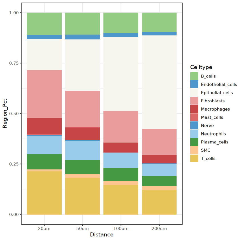
Result Visualization

Visualize proportions of surrounding cell types around target cell type

ggplot(neigh_freq1, aes(fill = Celltype, y = Region_Pct, x = Distance)) +
  theme_bw() +
  geom_bar(position = "fill", stat = "identity") +
  scale_fill_manual(
    values = c("#93cc82", "#4d97cd", "#f6f5ee", "#ea9c9d", "#c74546", 
               "#db6968", "#4d97cd", "#99cbeb", "#459943", 
               "#fdc58f", "#e8c559", "#a3d393", "#f8984e"), # Customize colors
    name = "Celltype"  # Custom legend name
  ) +
  theme(
    plot.title = element_text(hjust = 0.5),
    panel.background = element_blank()
  )

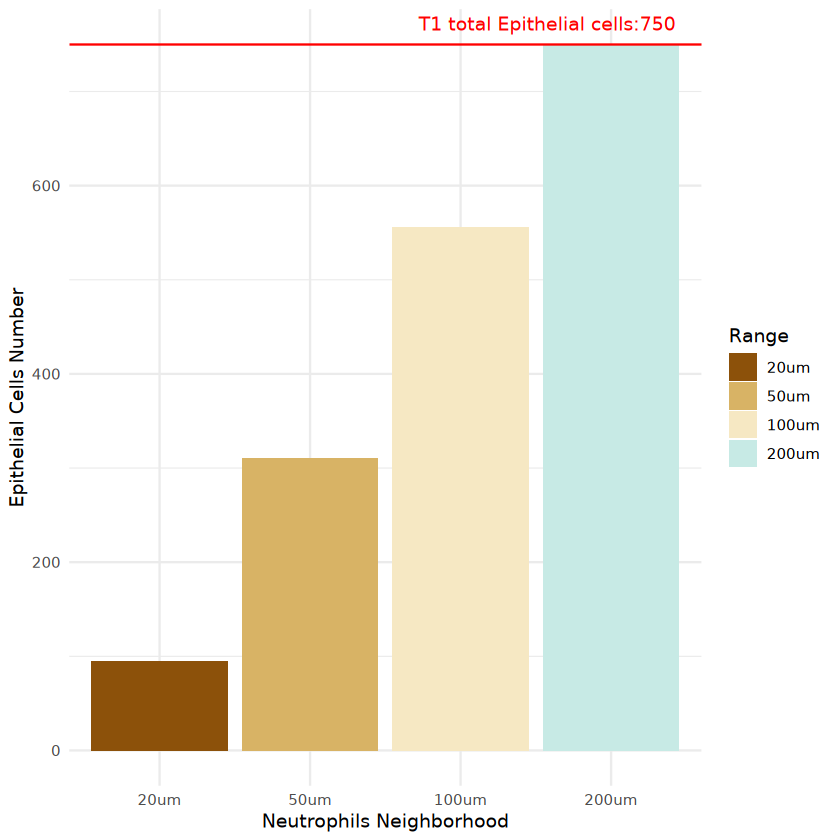
Visualize counts of specific surrounding cell types around target cell type

plot = neigh_freq1[neigh_freq1$Celltype %in% "T_cells",]
plot$Distance = factor(plot$Distance,levels = c("20um","50um","100um","200um"))

plot

A tibble: 4 × 4
Celltype	Cell_number	Distance	Region_Pct
<fct>	<int>	<fct>	<dbl>
T_cells	94	20um	21.26697
T_cells	310	50um	17.95020
T_cells	556	100um	14.52835
T_cells	750	200um	11.98274

ggplot(plot, aes(x = Distance, y = Cell_number, fill = Distance)) +
  geom_col() +  # Use geom_col() instead of geom_bar(stat="identity")
  scale_fill_manual(
    values = c("#8c510a", "#d8b365", "#f6e8c3", "#c7eae5"),
    name = "Range"  # Custom legend name
  ) +
  labs(
    x = "Neutrophils Neighborhood",  # x-axis label
    y = "Epithelial Cells Number",  # y-axis label
  ) +
  theme_minimal()+ # Use minimal theme
geom_hline(yintercept = 750,color="red")+
  annotate(
    "text", 
    x = Inf,  # Display on far right
    y = 750,
    label = "T1 total Epithelial cells:750", 
    color = "red",
    hjust = 1.1,  # Right align
    vjust = -1
  )

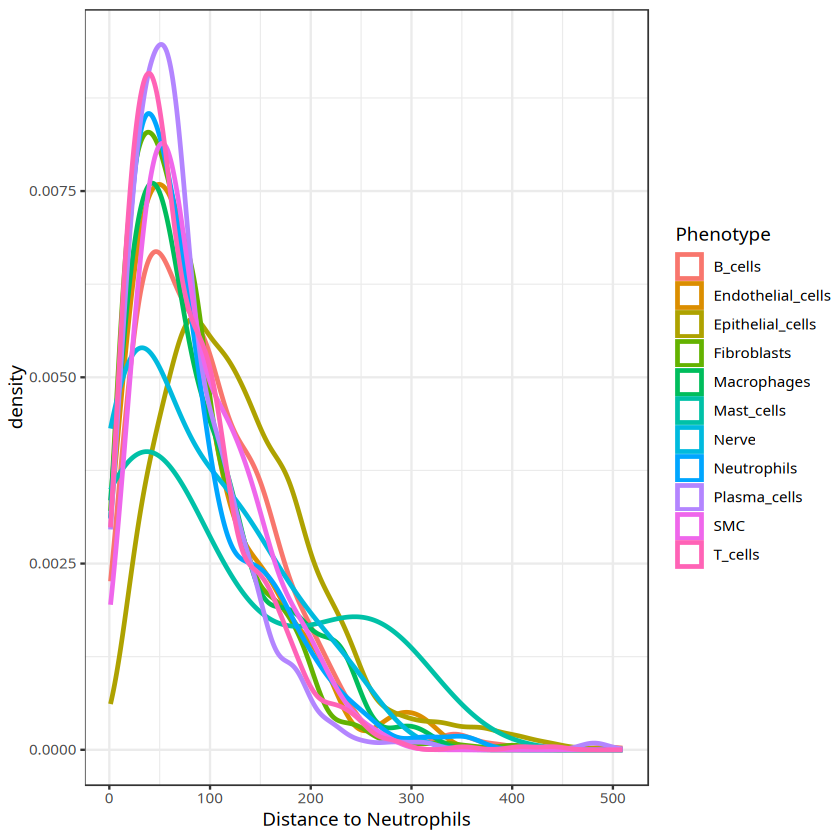
Visualize density distribution of cell types around target cell type

sub_position = rownames_to_column(sub_position,"Cell ID")
sub_position = cbind(sub_position,sub@meta.data[,col_celltype])
colnames(sub_position)[2:4] = c("Cell X Position","Cell Y Position","Phenotype")
sub_position

distances=find_nearest_distance(sub_position)
csd_with_distance=bind_cols(sub_position, distances)
ggplot(csd_with_distance,aes(`Distance to Neutrophils`, color=Phenotype))+geom_density(size=1)+theme_bw()

Single-cell Spatial Neighborhood Statistics: Spatial Distribution and Neighborhood Analysis ​

Load Analysis R Packages ​

Input Object Details ​

Read RDS and Metadata, Preprocess Data ​

Calculate Spatial Neighborhood Composition in 4 Ranges ​