SeekArc Single-cell Multi-omics (RNA+ATAC) Multi-sample Integration Tutorial

Author: SeekGene

Time: 25 min

Words: 4.9k words

Updated: 2026-02-28

Reads: 0 times

scATAC + RNA-seq Analysis Guide Notebooks Basic Analysis

Environment Preparation

Load R Packages

Please select the 'common_r' environment for this tutorial.

# Load required R packages
suppressPackageStartupMessages({
  library(Seurat)
  library(Signac)
  library(EnsDb.Hsapiens.v86, lib.loc = "/PROJ2/FLOAT/shumeng/apps/miniconda3/envs/python3.10/lib/R/library")
  library(BSgenome.Hsapiens.UCSC.hg38,lib = "/PROJ2/FLOAT/shumeng/apps/miniconda3/envs/python3.10/lib/R/library")
  library(biovizBase, lib = "/PROJ2/FLOAT/shumeng/apps/miniconda3/envs/python3.10/lib/R/library")
  #library(BSgenome.Mmusculus.UCSC.mm10)
  #library(EnsDb.Mmusculus.v79)
  library(dplyr)
  library(ggplot2)
  library(patchwork)
  library(harmony)
})

# Set random seed
set.seed(1234)

# Set Seurat options (Note: 8000 * 1024^2 is approx 8GB)
options(future.globals.maxSize = 8000 * 1024^2)  # 8GB

# Define color scheme
my36colors <-c( '#E5D2DD', '#53A85F', '#F1BB72', '#F3B1A0', '#D6E7A3', '#57C3F3', '#476D87',
                '#E95C59', '#E59CC4', '#AB3282', '#23452F', '#BD956A', '#8C549C', '#585658',
                '#9FA3A8', '#E0D4CA', '#5F3D69', '#C5DEBA', '#58A4C3', '#E4C755', '#F7F398',
                '#AA9A59', '#E63863', '#E39A35', '#C1E6F3', '#6778AE', '#91D0BE', '#B53E2B',
                '#712820', '#DCC1DD', '#CCE0F5', '#CCC9E6', '#625D9E', '#68A180', '#3A6963',
                '#968175', "#6495ED", "#FFC1C1",'#f1ac9d','#f06966','#dee2d1','#6abe83','#39BAE8','#B9EDF8','#221a12',
                '#b8d00a','#74828F','#96C0CE','#E95D22','#017890')

Get Gene Annotation Info

We will get genome annotation info (gene locations, transcripts, exons, TSS, etc.) from EnsDb. Change species as needed. Info is used for:

• Calculate ATAC TSS enrichment (check if open chromatin is concentrated near TSS)
• Construct gene activity matrix (map peak signals to genes)
• Peak annotation and functional analysis

Notes:

• Match species with reference genome version (e.g., EnsDb.Hsapiens.v86 for hg38, EnsDb.Mmusculus.v75 for mm10)
• Consistent chromosome naming (e.g., use 'chr1', 'chr2' prefixes)

# Get gene annotation info (suppress warnings/messages)
suppressWarnings({
  suppressMessages({
    annotation <- GetGRangesFromEnsDb(ensdb = EnsDb.Hsapiens.v86)
    seqlevels(annotation) <- paste0('chr', seqlevels(annotation))
    genome(annotation) <- 'hg38'
  })
})

Data Loading

This tutorial provides two data input methods. Choose the one that suits your needs:

Cloud Platform RDS File Loading

Data Characteristics:

• RDS files are standard Seurat object files
• Data has been preprocessed and samples merged
• Ready for downstream analysis; can also extract matrix for re-integration

Applicable Scenarios:

• When you cannot obtain standard filtered_feature_bc_matrix files
• When you want to learn by integrating existing cloud data
• When you need to quickly re-run scRNA-seq integration

Notes:

• Refer to Jupyter tutorial for data mounting and RDS reading

For example: /home/demo-SeekGene-com/workspace/data/AY1752565399550/

# Read data
input <- readRDS("/home/demo-seekgene-com/workspace/data/AY1752565399550/input.rds")
meta <- read.table("/home/demo-seekgene-com/workspace/data/AY1752565399550/meta.tsv", 
                  header = TRUE, 
                  sep = "\t", 
                  row.names = 1)

# Extract genome annotation (Signac lacks Annotation(); get from ChromatinAssay)
annotations <- input@assays$ATAC@annotation  # Ensure ATAC is ChromatinAssay

# Create Seurat object (RNA data)
data <- CreateSeuratObject(
    counts = input@assays$RNA@counts,
    meta.data = meta
)

# Create ChromatinAssay (ATAC data)
data[["ATAC"]] <- CreateChromatinAssay(
    counts = input@assays$ATAC@counts,
    fragments = input@assays$ATAC@fragments,
    annotation = annotations  # Add genome annotation
)

# Split data by sample
seurat_list <- SplitObject(data, split.by = "Sample")

# Clear memory
rm(data, input)
gc()

Standard filtered_XXXX_bc_matrix File Loading

Applicable Scenarios:

• When you have standard gene expression matrix and peaks matrix files
• When you want to independently complete SeekArc multi-omics integration and batch correction
• When you need a complete workflow from raw data to integration analysis

Note:

• Please ensure the file structure between samples is as follows:

Data directory structure requirements:

1. Folder name for each sample must be the Sample ID, e.g., S127, S44R.
2. Each sample folder must contain the following files:
   • filtered_feature_bc_matrix: scRNA-seq expression matrix folder, containing barcodes.tsv.gz, features.tsv.gz, and matrix.mtx.gz.
   • filtered_peaks_bc_matrix: ATAC peak matrix folder, containing barcodes.tsv.gz, features.tsv.gz, and matrix.mtx.gz.
   • {Sample ID}_A_fragments.tsv.gz: ATAC fragments file, e.g., S127_A_fragments.tsv.gz.
   • {Sample ID}_A_fragments.tsv.gz.tbi: ATAC fragments index file, e.g., S127_A_fragments.tsv.gz.tbi.

Specific folder structure as follows:

├── S127/
│ ├── filtered_feature_bc_matrix/ (scRNA-seq Expression Matrix)
│ │ ├── barcodes.tsv.gz
│ │ ├── features.tsv.gz
│ │ └── matrix.mtx.gz
│ ├── filtered_peaks_bc_matrix/ (ATAC Peak Matrix)
│ │ ├── barcodes.tsv.gz
│ │ ├── features.tsv.gz
│ │ └── matrix.mtx.gz
│ ├── S127_A_fragments.tsv.gz (ATAC Fragments File)
│ └── S127_A_fragments.tsv.gz.tbi
├── S44R/
│ ├── filtered_feature_bc_matrix/
│ │ ├── barcodes.tsv.gz
│ │ ├── features.tsv.gz
│ │ └── matrix.mtx.gz
│ ├── filtered_peaks_bc_matrix/
│ │ ├── barcodes.tsv.gz
│ │ ├── features.tsv.gz
│ │ └── matrix.mtx.gz
│ ├── S44R_A_fragments.tsv.gz
│ └── S44R_A_fragments.tsv.gz.tbi

sample_names <- c('S127', 'S44R')
# Create empty list to store Seurat objects
seurat_list <- list()

# Loop through each sample data
for(sample in sample_names){
  cat('Processing sample:', sample, '\n')
  
  # Build file path
  atac_path <- file.path(sample, 'filtered_peaks_bc_matrix')
  rna_path <- file.path(sample, 'filtered_feature_bc_matrix')
  frag_path <- file.path(sample, paste0(sample, '_A_fragments.tsv.gz'))

  # Read RNA data
  rna_counts <- Read10X(data.dir = rna_path)

  # Create Seurat object
  obj <- CreateSeuratObject(
    counts = rna_counts,
    assay = "RNA")
  
  obj$Sample <- sample
  rm(rna_counts)
  gc()
  
  # Read ATAC data
  atac_counts <- Read10X(data.dir = atac_path)
  atac_counts <- atac_counts[Matrix::rowSums(atac_counts > 0) >= 3, ]   
  
  ChromatinAssay <- CreateChromatinAssay(
    counts = atac_counts,
    sep = c(":", "-"),
    fragments = frag_path,
    annotation = annotation
  )
  
  obj[["ATAC"]] <- ChromatinAssay
  rm(atac_counts, ChromatinAssay)
  gc()
  
  # Add object to list
  seurat_list[[sample]] <- obj
  cat('Sample', sample, 'processing complete\n')
}

output

正在处理样本: S127


Computing hash



样本 S127 处理完成
正在处理样本: S44R


Computing hash



样本 S44R 处理完成

Data Quality Control

Calculate QC Metrics

RNA QC Metrics:

• percent.mt: Mitochondrial gene percentage (usually <20%)

ATAC QC Metrics:

• TSS.enrichment: TSS enrichment score (usually >2)
• nucleosome_signal: Nucleosome signal (lower is better)
• nCount_ATAC: Total ATAC counts (usually 1000-10000)
• nfeature_RNA: Total RNA features (usually 200-10000)

# Perform QC on each sample
suppressWarnings({
  suppressMessages({
      for(i in names(seurat_list)){
          # RNA QC metrics
          seurat_list[[i]][["percent.mt"]] <- PercentageFeatureSet(seurat_list[[i]], pattern = "^MT-")
          # ATAC QC metrics
          DefaultAssay(seurat_list[[i]]) <- "ATAC"
          # Calculate TSS enrichment score
          seurat_list[[i]] <- TSSEnrichment(object = seurat_list[[i]], fast = FALSE) 
          # Calculate nucleosome signal
          seurat_list[[i]] <- NucleosomeSignal(object = seurat_list[[i]])
      }
  })
})

QC Metrics Visualization

Use violin plots to view distribution/outliers of QC metrics to determine appropriate thresholds:

Suggestions:

• Look for obvious long tails or bimodal distributions
• Try multiple thresholds and compare if downstream clustering/UMAP is clearer

# Visualize QC metrics (optional execution)
options(repr.plot.width = 17, repr.plot.height = 10)
suppressWarnings({
for (sample_name in names(seurat_list)) {
  seurat_obj <- seurat_list[[sample_name]]
  p1=DensityScatter(seurat_obj, x = 'nCount_ATAC', y = 'TSS.enrichment', log_x = TRUE, quantiles = TRUE)
  p2=VlnPlot(
      object = seurat_obj,
      features = c('nCount_ATAC', 'TSS.enrichment',  'nucleosome_signal',"nFeature_RNA", "nCount_RNA", "percent.mt"),
      pt.size = 0.1,
      ncol = 6
  )
 print(p1 / p2 + plot_annotation(title = sample_name))
}
})

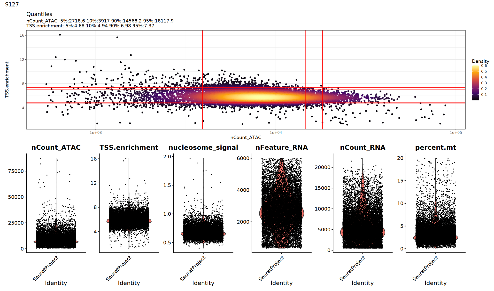
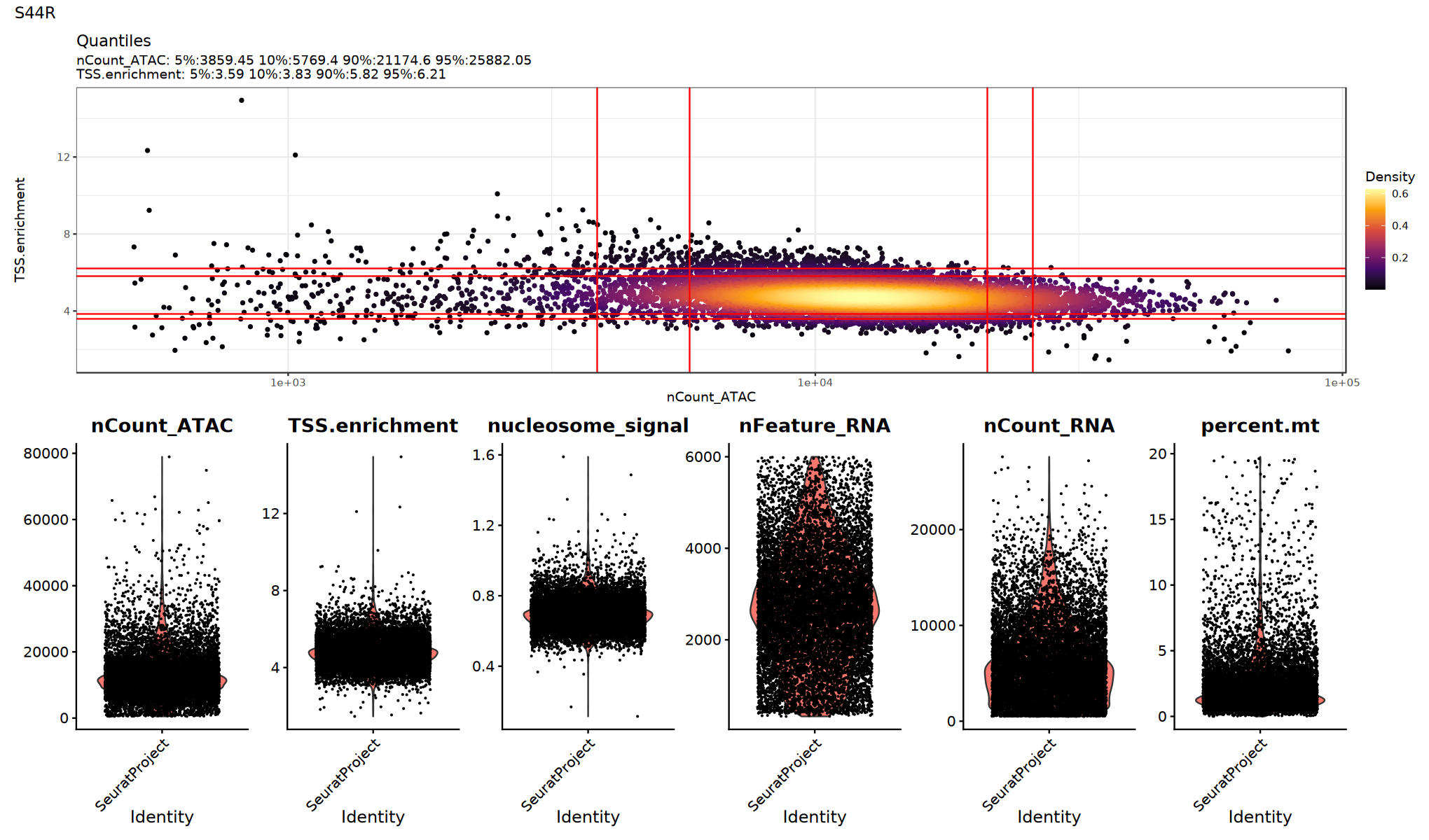
Filter Low-Quality Cells

Filter low-quality cells based on QC metrics. Thresholds should be adjusted based on data characteristics and violin plots above.

# QC Filtering
for(i in names(seurat_list)){
  cat('QC filtering for sample', i, '...\n')
  
  cells_before <- ncol(seurat_list[[i]])
  
  seurat_list[[i]] <- subset(
    seurat_list[[i]],
    subset = nFeature_RNA > 200 &
             nFeature_RNA < 6000 &
             nCount_RNA > 500 &
             nCount_RNA < 30000 &
             percent.mt < 20 &
             nCount_ATAC > 500 &
             nCount_ATAC < 100000 &
             TSS.enrichment > 1 &
             nucleosome_signal < 2
  )
  
  cells_after <- ncol(seurat_list[[i]])
  cat('Sample', i, 'filtering complete: Before', cells_before, 'cells, After', cells_after, 'cells\n')
}

output

正在对样本 S127 进行质控过滤...n 样本 S127 过滤完成: 过滤前 13957 个细胞，过滤后 12483 个细胞
正在对样本 S44R 进行质控过滤...n 样本 S44R 过滤完成: 过滤前 12072 个细胞，过滤后 10900 个细胞

Calculate Common Peaks Across Samples

Since peak calling is performed independently for each sample, peaks vary across samples. To integrate multiple samples, we must unify peak information and create a set of common peaks for all samples.

Workflow:

1. Merge peaks from all samples
2. Filter peak lengths (20bp-10kb)
3. Re-quantify common peaks for each sample

Notes: If you used the first data loading method (RDS) above, this part does not need to be analyzed.

Notes: If you used the first data loading method (RDS) above, this part does not need to be analyzed.

Notes: If you used the first data loading method (RDS) above, this part does not need to be analyzed.

# Extract peaks from all samples
all_peaks <- lapply(seurat_list, function(x) {
  DefaultAssay(x) <- "ATAC"
  granges(x@assays$ATAC)
})

# Merge all peaks
gr_list <- GRangesList(all_peaks)
all_granges <- unlist(gr_list, use.names = FALSE)
combined.peaks <- reduce(x = all_granges)

# Filter peak length
peakwidths <- width(combined.peaks)
common_peaks <- combined.peaks[peakwidths < 10000 & peakwidths > 20]

cat('Number of peaks after merging:', length(common_peaks), '\n')

# Create unified peak matrix for each sample
seurat_list <- lapply(seurat_list, function(x) {
  combined_counts <- FeatureMatrix(
    fragments = Fragments(x@assays$ATAC),
    features = common_peaks,
    cells = colnames(x)
  )
  
  combined_peaks_assay <- CreateChromatinAssay(
    counts = combined_counts,
    fragments = Fragments(x@assays$ATAC),
    annotation = Annotation(x@assays$ATAC)
  )
  
  # Add to Seurat object
  x[["combinedpeaks"]] <- combined_peaks_assay
  DefaultAssay(x) <- "combinedpeaks"
  x[["ATAC"]] <- NULL
  return(x)
})

output

合并后的peak数量: 211924


Extracting reads overlapping genomic regions

Extracting reads overlapping genomic regions

Multi-sample Merging

In multi-omics integration analysis, multi-sample merging is a key prerequisite.

Purpose of Merging:

• Merge data from multiple samples into a single Seurat object
• Prepare for subsequent batch correction and integration analysis
• Facilitate comparison with batch-corrected results

Important Notes:

• This step only performs simple data merging, not batch correction
• The merged object contains raw data from all samples
• Proceed with preprocessing steps like normalization, feature selection, PCA, and UMAP on merged data

# Merge all samples
suppressWarnings({
  suppressMessages({
      obj_merge <- merge(seurat_list[[1]], seurat_list[-1], merge.data = FALSE)
      DefaultAssay(obj_merge) <- "RNA" 
      obj_merge <- NormalizeData(obj_merge)
      obj_merge <- FindVariableFeatures(obj_merge, nfeatures = 2000)
      obj_merge <- ScaleData(obj_merge)
      obj_merge <- RunPCA(obj_merge)
      DefaultAssay(obj_merge) <- "combinedpeaks"
      obj_merge <- FindTopFeatures(obj_merge, min.cutoff = 10)
      obj_merge <- RunTFIDF(obj_merge)
      obj_merge <- RunSVD(obj_merge)
      obj_merge <- RunUMAP(obj_merge, reduction = "lsi", dims = 2:30,reduction.name="atacumap")
        })
})

Data Integration

Now we integrate SeekArc multi-omics data from multiple samples and perform dimensionality reduction and clustering. Two common methods for multi-omics integration are:

Integration Method Selection

CCA (Canonical Correlation Analysis) Integration:

• Integration based on Canonical Correlation Analysis
• Integrates by finding common variation patterns between samples
• Suitable for cases with large differences between samples
• Classic integration method in Seurat

Harmony Integration:

• Fast integration based on iterative clustering
• Corrects batch effects directly in reduced dimensional space
• High computational efficiency, suitable for large-scale data
• Preserves more biological variation

Method Selection Advice

• Harmony: Same platform different samples; faster for many samples or large datasets.
• CCA: Slower; recommended for severe batch effects, e.g., cross-platform data.

RNA Data Integration

Integrate Multi-sample RNA Data using CCA

# Switch to RNA assay
suppressWarnings({
  suppressMessages({
      objs <- lapply(seurat_list, function(x) {
          DefaultAssay(x) <- "RNA"
          return(x)
      })
      # Define CCA integration function
      integrate_cca <- function(objs) {
          # Use lapply instead of for loop
          objs <- lapply(objs, function(x) {
              x <- NormalizeData(x, verbose = FALSE)
              x <- FindVariableFeatures(x,nfeatures = 2000,selection.method = "vst")
              return(x)
          })
          features <- Seurat::SelectIntegrationFeatures(object.list = objs)
          anchors <- Seurat::FindIntegrationAnchors(
              object.list = objs,
              anchor.features = features
          ) 
          obj <- Seurat::IntegrateData(anchorset = anchors)
          DefaultAssay(obj) <- "integrated"
          obj <- ScaleData(obj, verbose = FALSE)
          obj <- RunPCA(obj, verbose = FALSE)
          obj <- RunUMAP(obj, reduction = "pca",reduction.name="rnaintegratedumap", dims = 1:30)
          #obj <- RunTSNE(obj, reduction = "pca", reduction.name="rnaintegratedtsne",dims = 1:30, check_duplicates = FALSE)
          return(obj)
      }
      # Execute CCA integration
      obj_integrated <- integrate_cca(seurat_list)
  })
})    
## Visualize RNA Data Batch Correction Effect
options(repr.plot.width=10, repr.plot.height=8)
DimPlot(obj_integrated, reduction = "rnaintegratedumap", group.by = "Sample")

Integrate Multi-sample RNA Data using Harmony

# RNA data integration function
integrate_harmony <- function(obj) {
  DefaultAssay(obj) <- "RNA"
  obj <- RunHarmony(obj, "Sample")
  obj <- RunUMAP(obj, reduction = "harmony",reduction.name="rnaharmonyumap",dims = 1:30)
  #obj <- RunTSNE(obj, reduction = "harmony",reduction.name="rnaharmonytsne",dims = 1:30,check_duplicates = FALSE)
  return(obj)
}
suppressWarnings({
  suppressMessages({
      obj_integrated = integrate_harmony(obj_merge)
              })
}) 
## Visualize RNA Data Batch Correction Effect
options(repr.plot.width=10, repr.plot.height=8)
DimPlot(obj_integrated, reduction = "rnaharmonyumap", group.by = "Sample")

ATAC Data Integration

Integrate Multi-sample ATAC Data using CCA

# Define ATAC integration function
options(future.globals.maxSize = 20 * 1024^3)
integrate_atac_cca <- function(object.list){
    object.list <- lapply(object.list, function(x) {
        DefaultAssay(x)="combinedpeaks"
        x=RunTFIDF(x)
        x=FindTopFeatures(x, min.cutoff = 5)
        x=RunSVD(x)
        return(x)
      })
    
    anchors <- FindIntegrationAnchors(
        object.list = object.list,
        anchor.features = rownames(obj_merge),
        reduction = "rlsi",
        dims = 2:30
    )
    
    integrated <- IntegrateEmbeddings(
            anchorset = anchors,
            reductions = obj_merge[["lsi"]],
            new.reduction.name = "integrated_lsi",
            dims.to.integrate = 1:30)
   integrated<- RunUMAP(integrated, reduction = "integrated_lsi", dims = 2:30,reduction.name="atacintegratedumap")
   #integrated<- RunTSNE(integrated, reduction = "integrated_lsi", dims = 2:30,reduction.name="atacintegratedtsne")
   return(integrated)
}

# Execute ATAC integration
suppressWarnings({
  suppressMessages({
      integrated_atac <- integrate_atac_cca(seurat_list)
  })
})  
# Add integrated dimensionality reduction results to main object
obj_integrated[['integrated_lsi']] <- integrated_atac[['integrated_lsi']]
obj_integrated[['atacintegratedumap']] <- integrated_atac[['atacintegratedumap']]
#obj_integrated[['atacintegratedtsne']] <- integrated_atac[['atacintegratedtsne']]
DefaultAssay(obj_integrated) <- "integrated"
# Visualize ATAC Batch Correction Effect
options(repr.plot.width=10, repr.plot.height=8)
DimPlot(obj_integrated, reduction = "atacintegratedumap", group.by = "Sample")

Integrate Multi-sample ATAC Data using Harmony

atac_integrate_harmony <- function(obj) {
  library(harmony)
  DefaultAssay(obj) <- "combinedpeaks"
  obj<- RunHarmony(
        object = obj,
        group.by.vars = 'Sample',
        reduction = 'lsi',
        assay.use = 'combinepeaks',
        reduction.save = "harmonylsi",
        project.dim = FALSE
        )
  obj <- RunUMAP(obj,reduction = 'harmonylsi',reduction.name="atacharmonyumap", dims = 2:30)
  #obj <- RunTSNE(obj, reduction = "harmonylsi",reduction.name="atacharmonytsne",dims = 2:50,check_duplicates = FALSE)
  return(obj)
}
suppressWarnings({
  suppressMessages({
      obj_integrated=atac_integrate_harmony(obj_integrated)
  })
})
# Visualize ATAC Batch Correction Effect
options(repr.plot.width=10, repr.plot.height=8)
DimPlot(obj_integrated, reduction = "atacharmonyumap", group.by = "Sample")

Weighted Nearest Neighbor (WNN) Analysis

WNN Principle

WNN method learns the relative importance of each data type (RNA and ATAC) and automatically assigns modality weights to each cell, thereby:

• Utilizing both RNA and ATAC information simultaneously
• Avoiding biases from a single modality
• Providing more accurate cell clustering and dimensionality reduction results

Parameter Description

• reduction.list: Specify dimensionality reduction results used for WNN
  • CCA Integration: list("pca", "integrated_lsi")
  • Harmony Integration: list("harmony", "harmonylsi")
• dims.list: Dimensions range used for each modality

# Find Multimodal Neighbors
suppressWarnings({
  suppressMessages({
      obj_integrated <- FindMultiModalNeighbors(
          object = obj_integrated,
          reduction.list = list("pca", "integrated_lsi"), # Select this for CCA method
          #reduction.list = list("harmony", "harmonylsi"), # Select this for Harmony method
          dims.list = list(1:30, 2:50),
          modality.weight.name = "RNA.weight",
          verbose = TRUE)
      # UMAP Dimensionality Reduction Based on WNN
      obj_integrated <- RunUMAP(
          object = obj_integrated,
          nn.name = "weighted.nn",
          assay = "RNA",
          verbose = TRUE,
          reduction.name = "wnnintergratedumap"
      )
  })
})

Clustering Analysis

Three Clustering Strategies

1. RNA Clustering: Based on gene expression similarity
2. ATAC Clustering: Based on chromatin accessibility similarity
3. WNN Clustering: Integrating two modalities (Recommended)

Result Interpretation

• Different methods may yield different clustering results
• WNN clustering usually discovers finer cell subpopulations
• It is recommended to prioritize WNN results for downstream analysis

Parameter Description Below

When performing clustering analysis below, please select the corresponding dimensionality reduction parameters based on the batch correction method used previously:

​​CCA Batch Removal​​:

• RNA Clustering: Use reduction="pca" in FindNeighbors

• ATAC Clustering: Use reduction="integrated_lsi" in FindNeighbors

​​Harmony Batch Removal​​:

• RNA Clustering: Use reduction="harmony" in FindNeighbors

• ATAC Clustering: Use reduction="harmonylsi" in FindNeighbors

suppressWarnings({
  suppressMessages({
      # RNA Clustering
      obj_integrated <- FindNeighbors(object = obj_integrated, reduction = 'pca',graph.name = "rnaneigobr", dims = 1:30)
      #obj_integrated <- FindNeighbors(object = obj_integrated, reduction = 'harmony', dims = 1:30)
      obj_integrated <- FindClusters(object = obj_integrated, verbose = FALSE,graph.name = "rnaneigobr", algorithm = 3, resolution = 0.5)
      # ATAC Clustering
      obj_integrated <- FindNeighbors(object = obj_integrated, reduction = 'integrated_lsi', graph.name = "atacneigobr", dims = 2:30)
      #obj_integrated <- FindNeighbors(object = obj_integrated, reduction = 'harmonylsi', graph.name = "atacneigobr", dims = 2:30)
      obj_integrated <- FindClusters(object = obj_integrated, verbose = FALSE, graph.name = "atacneigobr",resolution = 0.5, algorithm = 3)
      # WNN Clustering
      obj_integrated <- FindClusters(obj_integrated, graph.name = "wknn", algorithm = 3, resolution = 0.5, verbose = TRUE)
        })
})

output

Computing nearest neighbor graph

Computing SNN

Computing nearest neighbor graph

Computing SNN

Only one graph name supplied, storing nearest-neighbor graph only

Warning message:
"The following arguments are not used: cluster.name"

Warning message:
"The following arguments are not used: cluster.name"

Visualization Parameter Description

Dimensionality Reduction Visualization Consistency Requirements When visualizing clustering results, please ensure the UMAP dimensionality reduction method used is consistent with the previous clustering analysis:

​​CCA Batch Removal​​:

• RNA Clustering Results: Use "rnaintegratedumap" reduction space

• ATAC Clustering Results: Use "atacintegratedumap" reduction space

• WNN Clustering Results: Use "wnnintergratedumap" reduction space

​​Harmony Batch Removal​​:

• RNA Clustering Results: Use "rnaharmonyumap" reduction space

• ATAC Clustering Results: Use "atacharmonyumap" reduction space

• WNN Clustering Results: Use "wnnintergratedumap" reduction space

# Compare Clustering Results of Different Methods
p1 <- DimPlot(obj_integrated, reduction = "rnaintegratedumap", group.by = "rnaneigobr_res.0.5",label=T, cols = my36colors) + ggtitle("RNA")
p2 <- DimPlot(obj_integrated, reduction = "atacintegratedumap", group.by = "atacneigobr_res.0.5",label=T, cols = my36colors) + ggtitle("ATAC")
p3 <- DimPlot(obj_integrated, reduction = "wnnintergratedumap", group.by = "wknn_res.0.5",label=T, cols = my36colors) + ggtitle("WNN")


#p1 <- DimPlot(obj_integrated, reduction = "rnaharmonyumap", group.by = "rnaneigobr_res.0.5",label=T, cols = my36colors) + ggtitle("RNA")
#p2 <- DimPlot(obj_integrated, reduction = "atacharmonyumap", group.by = "atacneigobr_res.0.5",label=T, cols = my36colors) + ggtitle("ATAC")
#p3 <- DimPlot(obj_integrated, reduction = "wnnintergratedumap", group.by = "wknn_res.0.5",label=T, cols = my36colors) + ggtitle("WNN")
options(repr.plot.width=23, repr.plot.height=6)
print(p1 + p2 + p3)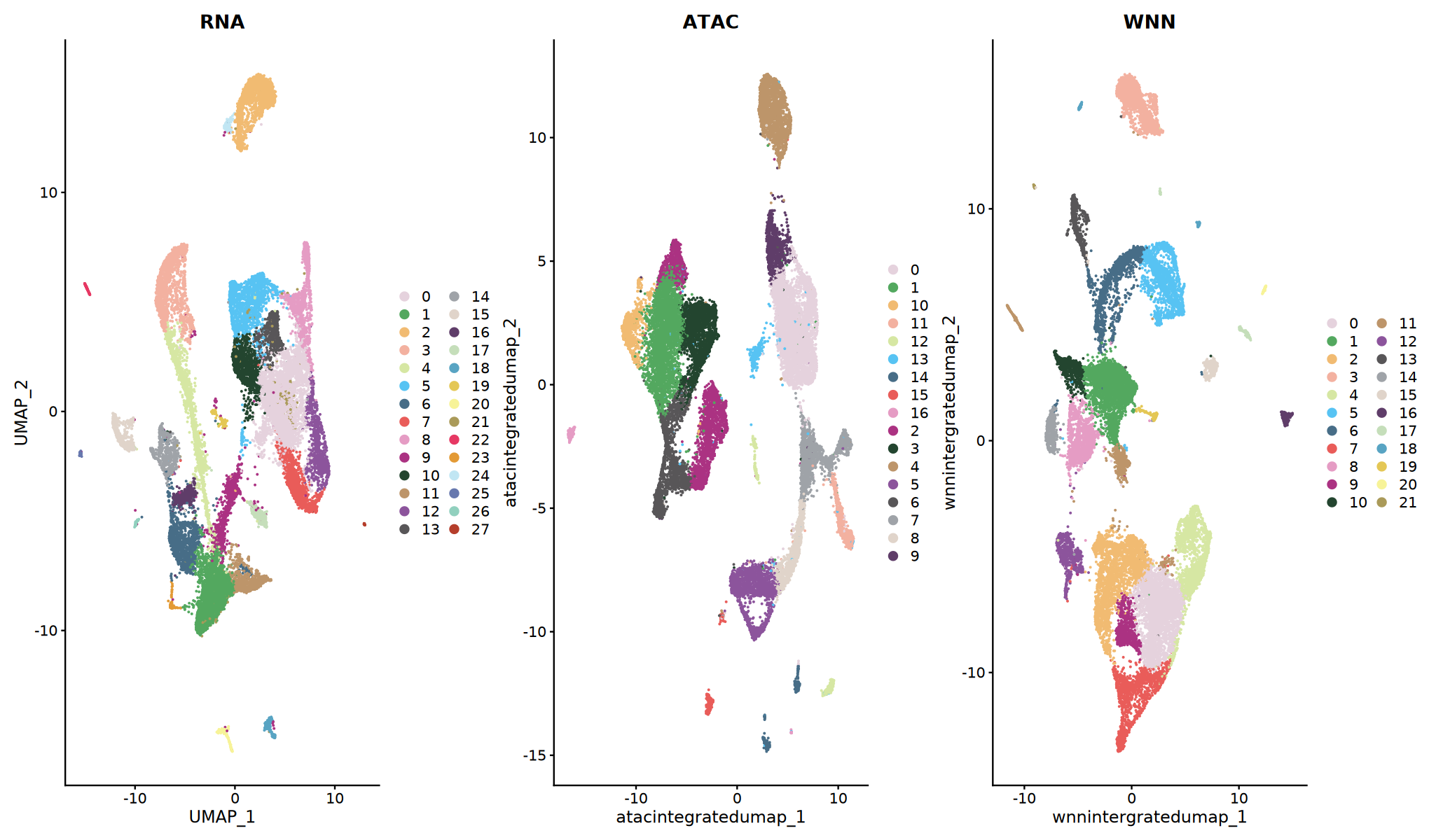

Cell Type Annotation

Marker Genes

Collect marker gene sets for different cell types based on tissue type. This example data is from eye. Below are eye cell types and their corresponding marker genes. Use DotPlot to visualize which cell type markers are highly expressed in different clusters.

eye_marker_integrated <- list(
  # ========== Photoreceptor Cells ==========
  "Rod_Photoreceptors" = c("RHO", "PDE6B", "CNGB1", "PDE6A", "NR2E3", "REEP6",
                          "RCVRN", "SAG", "NEB", "SLC24A3", "TRPM1"),
  "Cone_Photoreceptors" = c("ARR3", "GNAT2", "OPN1SW", "TRPM3"),

  # ========== Retinal Neurons ==========
  "Bipolar_Cells" = c("VSX1", "OTX2", "GRM6", "PRKCA",
                     "DLG2", "NRXN3", "RBFOX3", "FSTL4"),
  "Amacrine_Cells" = c("GAD1", "GAD2", "C1QL2", "TFAP2B", "SLC32A1"),
  "Horizontal_Cells" = c("ONECUT1", "LHX1", "CALB1", "NFIA"),
  "Retinal_Ganglion_Cells" = c("RBPMS", "THY1", "NEFL", "POU4F2"),

  # ========== Glial Cells ==========
  "Muller_Glia" = c("SLC1A3", "RLBP1", "SOX9", "CRYAB"),
  "Astrocytes" = c("GFAP", "AQP4", "S100B"),
  "Microglia" = c("TMEM119", "C1QA", "AIF1", "CX3CR1", "CD74",
                 "PTPRC", "CSF1R", "CCL3L1", "SPP1", "P2RY12"),

  # ========== Vascular and Support Cells ==========
  "Endothelial" = c("FLT1", "PODXL", "PLVAP", "KDR", "EGFL7",
                   "CLDN5", "PECAM1", "CDH5"),
  "Pericytes" = c("PDGFRB", "RGS5", "CSPG4", "STAB1"),

  # ========== Epithelial Cells ==========
  "RPE" = c("RPE65", "BEST1", "PMEL", "TYRP1", "DCT", "SLC38A11"),
  #"Corneal_Epithelial" = c("KRT12", "KRT3"),
  "Corneal_Endothelial" = c("SLC4A11", "COL8A2", "ATP1A1"),
  "Conjunctival_Epithelial" = c("KRT13", "KRT19", "MUC5AC"),
  "Retinal_Progenitors" = c("VSX2", "PAX6","SOX2", "HES1", "NOTCH1"),  # Neural Retina Progenitors

  # ========== Lens Cells ==========
  "Lens_Epithelial" = c("CRYAA", "BFSP1", "MIP"),
  "Lens_Fiber" = c("CRYGS", "LIM2", "FN1"),

  # ========== Other Cells ==========
  "Melanocytes" = c("TYR", "MLANA", "MITF"),
  #"Erythrocytes" = c("HBB", "HBA1", "HBA2"),
  "ECM" = c("COL1A1", "COL3A1", "COL12A1", "COL1A2", "COL6A3")#,
  #"Others" = c("TTN", "CLCN5", "DCC", "MIAT")
)

# Set Figure Size
options(repr.plot.width=25, repr.plot.height=7)

# Plot DotPlot
DefaultAssay(obj_integrated)="RNA"
DotPlot(obj_integrated, 
        group.by = "wknn_res.0.5", 
        features = eye_marker_integrated,
        cols = c("#f8f8f8","#ff3472"),
       #dot.min = 0.05,
       dot.scale = 8)+  # Apply custom color scheme
  RotatedAxis() + 
  scale_x_discrete("") + 
  scale_y_discrete("") +
  theme(
    axis.text.x = element_text(size = 12, face = "bold", 
                              angle = 45, hjust = 1, vjust = 1),
    axis.text.y = element_text(size = 12, face = "bold"),
    plot.title = element_text(size = 14, face = "bold", hjust = 0.5),
    legend.title = element_text(size = 10, face = "bold")
  ) +
  ggtitle("Marker Genes Expression") +
  labs(color = "Expression\nLevel")  # Modify legend title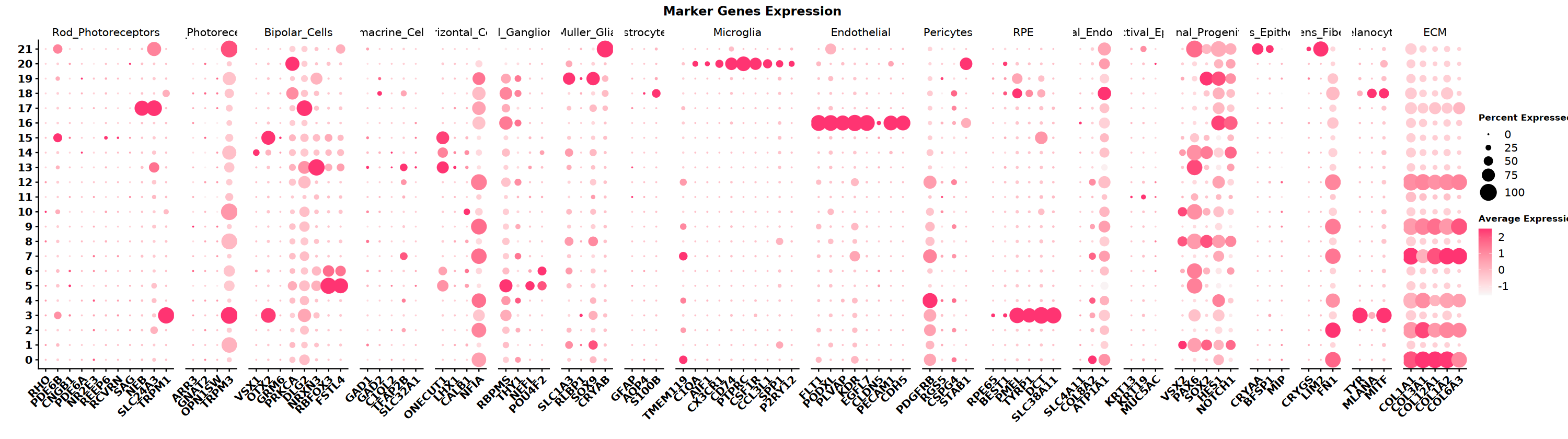

** Notes ** SeekArc single-cell dual-omics cell annotation is generally based on wnn multimodal dimensionality reduction, annotating based on marker gene expression in wknn clustering results.

options(repr.plot.width=10, repr.plot.height=8)
DimPlot(obj_integrated, reduction = "wnnintergratedumap", group.by = "wknn_res.0.5", cols = my36colors,label = T)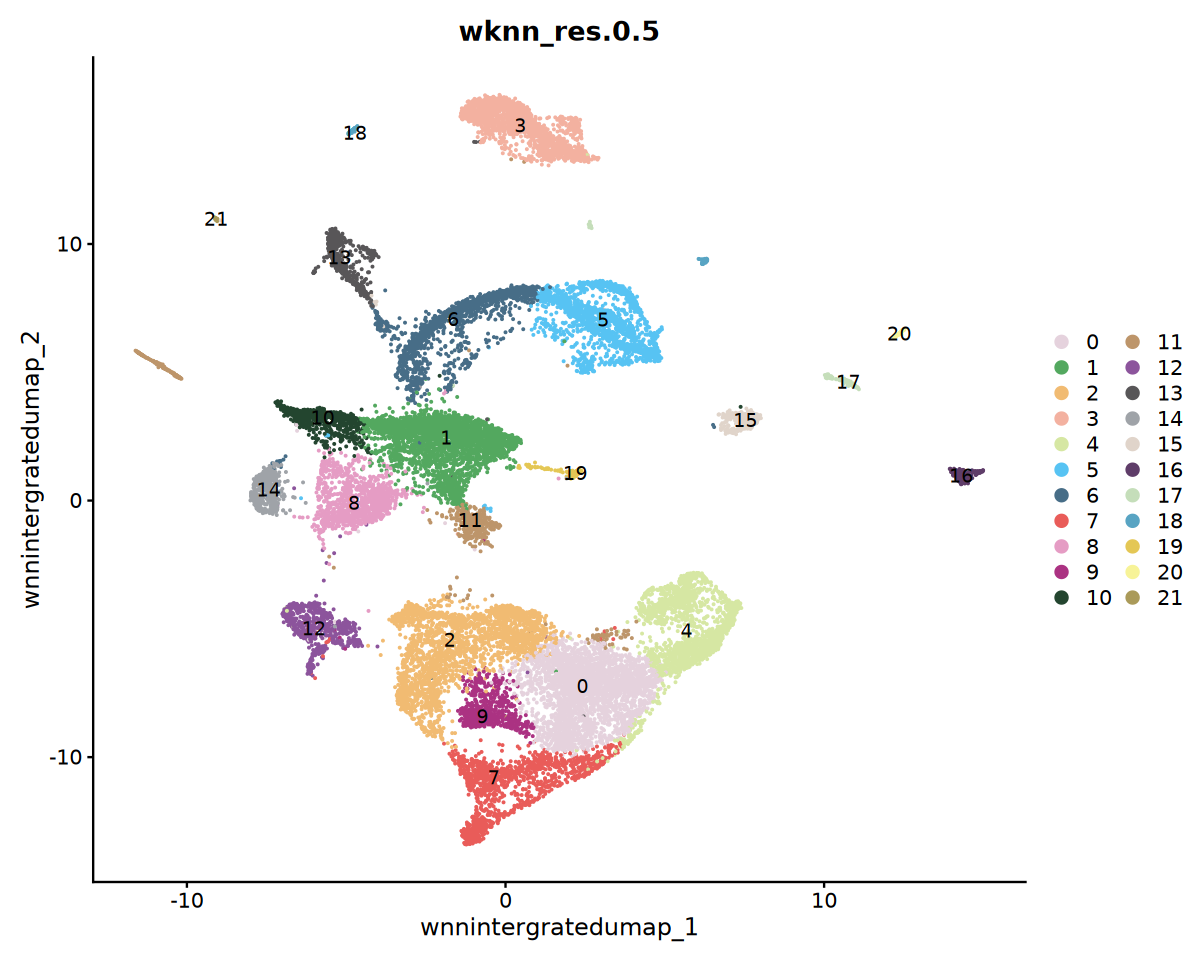

Cell Type Labeling

cat('Starting cell type annotation...', Sys.time(), '\n')

# Annotate cell types based on clustering results (needs adjustment based on actual marker gene expression)
# Here is an example, adjust based on DotPlot results in practice
celltype_mapping <- c(
  "0" = "ECM",
  "1" = "Retinal_Progenitors",
  "2" = "ECM",
  "3" = "PRE",
  "4" = "ECM",
  "5" = "Bipolar_Cells",
  "6" = "Bipolar_Cells",
  "7" = "ECM",
  "8" = "Retinal_Progenitors",
  "9" = "ECM",
  "10" = "Retinal_Progenitors",
  "11" = "Conjunctival_Epithelial",
  "12" = "ECM",
  "13" = "Bipolar_Cells",
  "14" = "Retinal_Progenitors",
  "15" = "Doublets",
  "16" = "Endothelial",
  "17" = "Rod_Photoreceptors",
  "18" = "Astrocytes",
  "19" = "Muller_Glia",
  "20" = "Microglia",
  "21" = "Lens"
)

# Apply Cell Type Annotation
obj_integrated$celltype <- recode(
  obj_integrated$wknn_res.0.5,
  !!!celltype_mapping
)

output

开始细胞类型注释... 1754902885

Visualization of Annotation Results

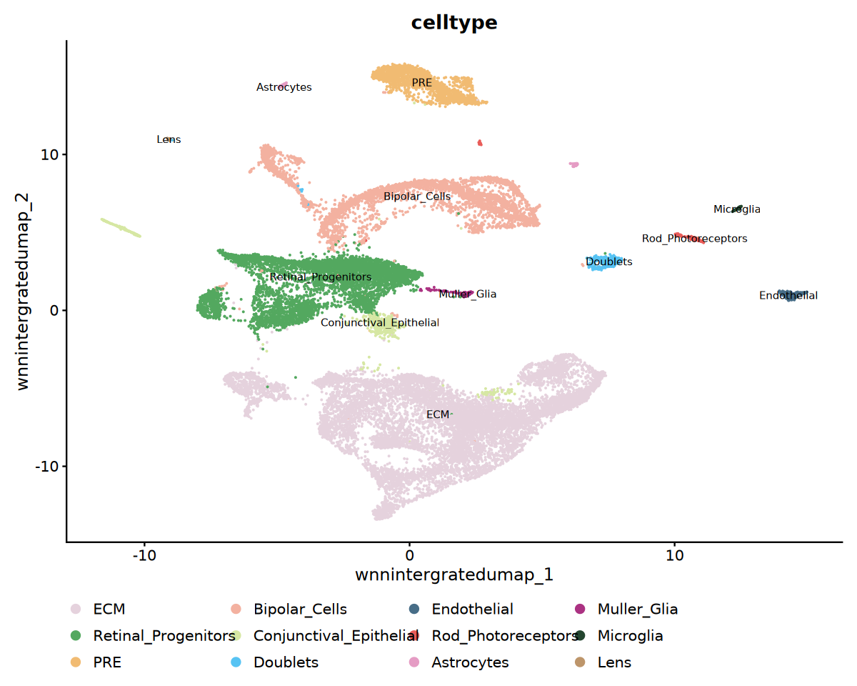
cat('Visualizing cell type annotation...', '\n')

# Cell Type UMAP Visualization
p1 <- DimPlot(
  obj_integrated,
  reduction = "wnnintergratedumap",
  group.by = "celltype",
  label = TRUE,
  label.size = 3,
  cols = my36colors
) +
  ggtitle("celltype") +
  theme(legend.position = "bottom")

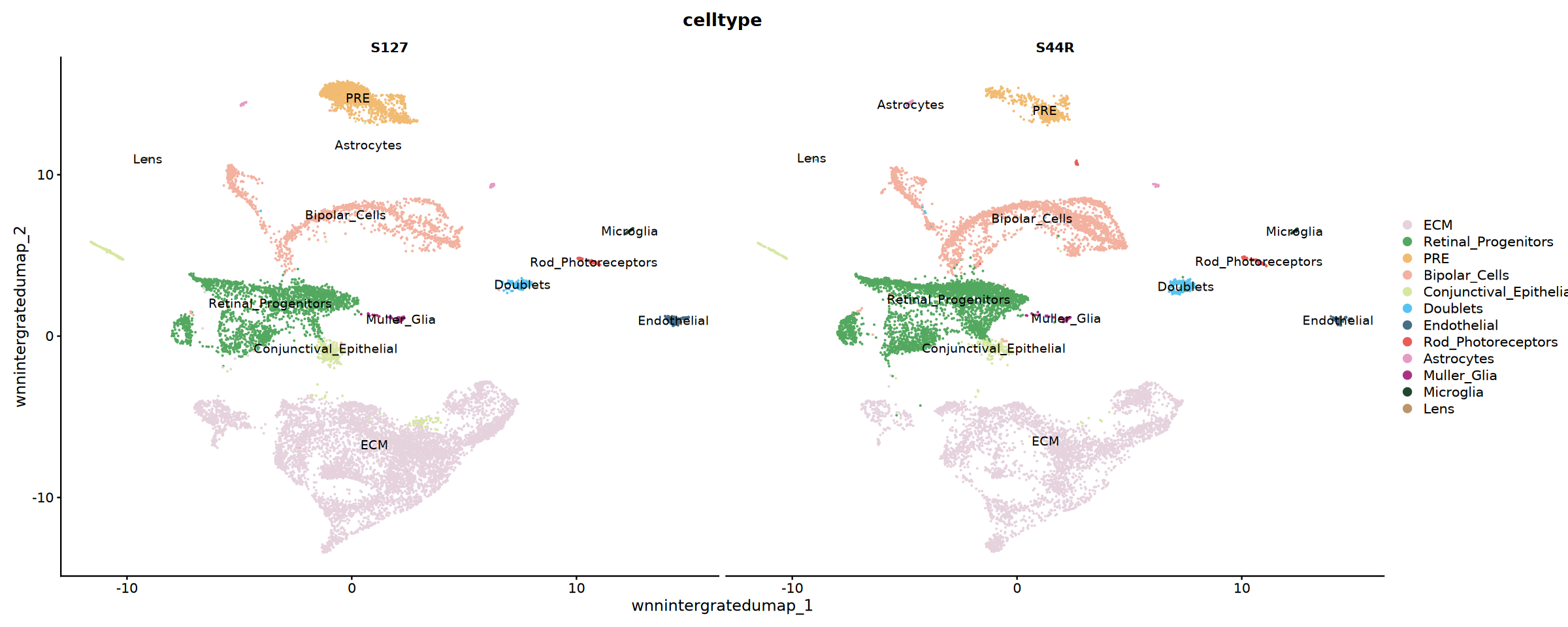
# Display Cell Type Distribution by Sample
p2 <- DimPlot(
  obj_integrated,
  reduction = "wnnintergratedumap",
  group.by = "celltype",
  split.by = "Sample",
  cols = my36colors,
  ncol = 2,label=T
) 

# Save Cell Type Annotation Plot
pdf("celltype_annotation.pdf", width = 16, height = 12)
print(p1)
print(p2)
dev.off()
options(repr.plot.width=10, repr.plot.height=8)
print(p1)
options(repr.plot.width=20, repr.plot.height=8)
print(p2)

cat('Cell type annotation results unfolded by sample!', '\n')

output

细胞类型注释可视化...

pdf: 2

细胞类型注释结果分样本展开! 

Save Results

# Save Integrated Seurat Object
saveRDS(obj_integrated, file = "scMultiomics_integrated.rds")

Summary

This tutorial demonstrated the complete integration analysis workflow for single-cell multi-omics data.

Key Points

• Data Quality: Multi-omics data requires considering both RNA and ATAC QC metrics.
• Feature Unification: Peak merging ensures feature consistency across samples.
• Method Selection: Choose CCA or Harmony method based on data characteristics.
• Modality Integration: WNN method can fully utilize multimodal information.

Common Issues

• Insufficient Memory: Reduce dimensions used or lower resolution.
• Poor integration: Try adjusting parameters or Change integration method
• Suboptimal Clustering: Adjust resolution parameters or use different clustering algorithms.

Future Analysis Directions

• Cell type annotation and marker gene identification
• Differential expression gene and differential accessibility analysis
• Gene regulatory network inference
• Developmental trajectory and pseudotime analysis

sessionInfo()

output

R version 4.3.3 (2024-02-29)
Platform: x86_64-conda-linux-gnu (64-bit)
Running under: Debian GNU/Linux 12 (bookworm)

Matrix products: default
BLAS/LAPACK: /jp_envs/envs/common/lib/libopenblasp-r0.3.29.so; LAPACK version 3.12.0

locale:
[1] LC_CTYPE=C.UTF-8 LC_NUMERIC=C LC_TIME=C.UTF-8
[4] LC_COLLATE=C.UTF-8 LC_MONETARY=C.UTF-8 LC_MESSAGES=C.UTF-8
[7] LC_PAPER=C.UTF-8 LC_NAME=C LC_ADDRESS=C
[10] LC_TELEPHONE=C LC_MEASUREMENT=C.UTF-8 LC_IDENTIFICATION=C

time zone: Asia/Shanghai
tzcode source: system (glibc)

attached base packages:
[1] stats4 stats graphics grDevices utils datasets methods
[8] base

other attached packages:
[1] harmony_1.2.3 Rcpp_1.0.14
[3] patchwork_1.3.0 ggplot2_3.5.2
[5] dplyr_1.1.4 biovizBase_1.50.0
[7] BSgenome.Hsapiens.UCSC.hg38_1.4.5 BSgenome_1.70.1
[9] rtracklayer_1.62.0 BiocIO_1.12.0
[11] Biostrings_2.70.1 XVector_0.42.0
[13] EnsDb.Hsapiens.v86_2.99.0 ensembldb_2.26.0
[15] AnnotationFilter_1.26.0 GenomicFeatures_1.54.1
[17] AnnotationDbi_1.64.1 Biobase_2.62.0
[19] GenomicRanges_1.54.1 GenomeInfoDb_1.38.1
[21] IRanges_2.36.0 S4Vectors_0.40.2
[23] BiocGenerics_0.48.1 Signac_1.10.0
[25] SeuratObject_4.1.4 Seurat_4.4.0
[27] repr_1.1.7

loaded via a namespace (and not attached):
[1] RcppAnnoy_0.0.22 splines_4.3.3
[3] later_1.4.2 pbdZMQ_0.3-13
[5] bitops_1.0-9 filelock_1.0.3
[7] tibble_3.2.1 polyclip_1.10-7
[9] rpart_4.1.23 XML_3.99-0.17
[11] lifecycle_1.0.4 globals_0.16.3
[13] lattice_0.22-7 MASS_7.3-60.0.1
[15] backports_1.5.0 magrittr_2.0.3
[17] rmarkdown_2.29 Hmisc_5.2-1
[19] plotly_4.10.4 yaml_2.3.10
[21] httpuv_1.6.15 sctransform_0.4.1
[23] sp_2.2-0 spatstat.sparse_3.1-0
[25] reticulate_1.42.0 cowplot_1.1.3
[27] pbapply_1.7-2 DBI_1.2.3
[29] RColorBrewer_1.1-3 abind_1.4-5
[31] zlibbioc_1.48.0 Rtsne_0.17
[33] purrr_1.0.4 RCurl_1.98-1.16
[35] nnet_7.3-19 VariantAnnotation_1.48.1
[37] rappdirs_0.3.3 GenomeInfoDbData_1.2.11
[39] ggrepel_0.9.6 irlba_2.3.5.1
[41] listenv_0.9.1 spatstat.utils_3.1-3
[43] goftest_1.2-3 spatstat.random_3.3-3
[45] fitdistrplus_1.2-2 parallelly_1.43.0
[47] DelayedArray_0.28.0 leiden_0.4.3.1
[49] codetools_0.2-20 RcppRoll_0.3.1
[51] xml2_1.3.6 tidyselect_1.2.1
[53] farver_2.1.2 matrixStats_1.5.0
[55] BiocFileCache_2.10.1 base64enc_0.1-3
[57] spatstat.explore_3.4-2 GenomicAlignments_1.38.0
[59] jsonlite_2.0.0 Formula_1.2-5
[61] progressr_0.15.1 ggridges_0.5.6
[63] survival_3.8-3 tools_4.3.3
[65] progress_1.2.3 ica_1.0-3
[67] glue_1.8.0 SparseArray_1.2.2
[69] gridExtra_2.3 xfun_0.50
[71] MatrixGenerics_1.14.0 IRdisplay_1.1
[73] withr_3.0.2 fastmap_1.2.0
[75] digest_0.6.37 R6_2.6.1
[77] mime_0.13 colorspace_2.1-1
[79] scattermore_1.2 tensor_1.5
[81] dichromat_2.0-0.1 spatstat.data_3.1-6
[83] biomaRt_2.58.0 RSQLite_2.3.9
[85] tidyr_1.3.1 generics_0.1.3
[87] data.table_1.17.0 S4Arrays_1.2.0
[89] prettyunits_1.2.0 httr_1.4.7
[91] htmlwidgets_1.6.4 uwot_0.2.3
[93] pkgconfig_2.0.3 gtable_0.3.6
[95] blob_1.2.4 lmtest_0.9-40
[97] htmltools_0.5.8.1 ProtGenerics_1.34.0
[99] scales_1.3.0 png_0.1-8
[101] spatstat.univar_3.1-2 rstudioapi_0.15.0
[103] knitr_1.49 reshape2_1.4.4
[105] rjson_0.2.23 uuid_1.2-1
[107] checkmate_2.3.2 nlme_3.1-168
[109] curl_6.0.1 zoo_1.8-14
[111] cachem_1.1.0 stringr_1.5.1
[113] KernSmooth_2.23-26 parallel_4.3.3
[115] miniUI_0.1.1.1 foreign_0.8-87
[117] restfulr_0.0.15 pillar_1.10.2
[119] grid_4.3.3 vctrs_0.6.5
[121] RANN_2.6.2 promises_1.3.2
[123] dbplyr_2.5.0 xtable_1.8-4
[125] cluster_2.1.8.1 htmlTable_2.4.3
[127] evaluate_1.0.3 cli_3.6.4
[129] compiler_4.3.3 Rsamtools_2.18.0
[131] rlang_1.1.5 crayon_1.5.3
[133] future.apply_1.11.3 plyr_1.8.9
[135] stringi_1.8.7 viridisLite_0.4.2
[137] deldir_2.0-4 BiocParallel_1.36.0
[139] munsell_0.5.1 lazyeval_0.2.2
[141] spatstat.geom_3.3-6 Matrix_1.6-5
[143] IRkernel_1.3.2 hms_1.1.3
[145] bit64_4.5.2 future_1.40.0
[147] KEGGREST_1.42.0 shiny_1.10.0
[149] SummarizedExperiment_1.32.0 ROCR_1.0-11
[151] igraph_2.0.3 memoise_2.0.1
[153] fastmatch_1.1-6 bit_4.5.0.1