SeekSpace Advanced Analysis: Spatial Gene Expression Density Plotting
Time: 16 min
Words: 3.1k words
Updated: 2026-02-28
Reads: 0 times
python
import numpy as np
import pandas as pd
import matplotlib.pyplot as plt
from scipy.stats import gaussian_kde
from mpl_toolkits.mplot3d import Axes3D
Data Loading
First use R to save spatial coordinates and annotation results from rds
Read Gene Expression Matrix
python
celltype_df_all1 = pd.read_csv("/PROJ2/FLOAT/weichendan/seekspace/SGS2401017/updata_allsamples/10Density/26samples_IGF2_marker.csv")python
celltype_df_all1| cell_id | sample_id | IGF2 | IGF1R | IGF2R | IGF2_marker | IGF1R_marker | IGF2R_marker | |
|---|---|---|---|---|---|---|---|---|
| 0 | AAGTACCATGTATGATGTAGTCATACG | WTH1051 | 0.000000 | 1.337767 | 0.000000 | non_IGF2 | IGF1R | non_IGF2R |
| 1 | AAGTTCGATGCGCATCCAAGGCACTAT | WTH1051 | 0.000000 | 0.000000 | 0.000000 | non_IGF2 | non_IGF1R | non_IGF2R |
| 2 | ACAAGCTATGGTCATCTGGACTGTGGA | WTH1051 | 0.000000 | 0.000000 | 0.000000 | non_IGF2 | non_IGF1R | non_IGF2R |
| 3 | ACCCTTGTACAAGTCATCTAAGTACGA | WTH1051 | 0.000000 | 0.000000 | 0.000000 | non_IGF2 | non_IGF1R | non_IGF2R |
| 4 | ACTACGATACCGAGTGCGCTCTGCTTC | WTH1051 | 0.000000 | 1.340361 | 0.000000 | non_IGF2 | IGF1R | non_IGF2R |
| ... | ... | ... | ... | ... | ... | ... | ... | ... |
| 394417 | GTATTTCGCTGTAGAATGCTCTGCTTC | Normal_5 | 0.000000 | 0.249231 | 0.000000 | non_IGF2 | IGF1R | non_IGF2R |
| 394418 | TGAGGTTGCTCGAGTTTGCTCTGCTTC | Normal_5 | 4.161886 | 0.000000 | 0.445782 | IGF2 | non_IGF1R | IGF2R |
| 394419 | ATTCCCGATGCAACTGATAGTCATACG | Normal_5 | 3.798390 | 0.000000 | 0.192101 | IGF2 | non_IGF1R | IGF2R |
| 394420 | TTGCATTATGCGCTTCGTTCTGCGCTC | Normal_5 | 3.657890 | 0.000000 | 0.119740 | IGF2 | non_IGF1R | IGF2R |
| 394421 | CAAGCTAGCTGAGAATTCCTAATAACG | Normal_5 | 3.714930 | 0.108064 | 0.108064 | IGF2 | IGF1R | IGF2R |
394422 rows × 8 columns
python
celltype_df_all = celltype_df_all1.drop(columns=celltype_df_all1.columns[5:8])python
celltype_df_all| cell_id | sample_id | IGF2 | IGF1R | IGF2R | |
|---|---|---|---|---|---|
| 0 | AAGTACCATGTATGATGTAGTCATACG | WTH1051 | 0.000000 | 1.337767 | 0.000000 |
| 1 | AAGTTCGATGCGCATCCAAGGCACTAT | WTH1051 | 0.000000 | 0.000000 | 0.000000 |
| 2 | ACAAGCTATGGTCATCTGGACTGTGGA | WTH1051 | 0.000000 | 0.000000 | 0.000000 |
| 3 | ACCCTTGTACAAGTCATCTAAGTACGA | WTH1051 | 0.000000 | 0.000000 | 0.000000 |
| 4 | ACTACGATACCGAGTGCGCTCTGCTTC | WTH1051 | 0.000000 | 1.340361 | 0.000000 |
| ... | ... | ... | ... | ... | ... |
| 394417 | GTATTTCGCTGTAGAATGCTCTGCTTC | Normal_5 | 0.000000 | 0.249231 | 0.000000 |
| 394418 | TGAGGTTGCTCGAGTTTGCTCTGCTTC | Normal_5 | 4.161886 | 0.000000 | 0.445782 |
| 394419 | ATTCCCGATGCAACTGATAGTCATACG | Normal_5 | 3.798390 | 0.000000 | 0.192101 |
| 394420 | TTGCATTATGCGCTTCGTTCTGCGCTC | Normal_5 | 3.657890 | 0.000000 | 0.119740 |
| 394421 | CAAGCTAGCTGAGAATTCCTAATAACG | Normal_5 | 3.714930 | 0.108064 | 0.108064 |
394422 rows × 5 columns
python
celltype_df_all = celltype_df_all.set_index('cell_id')Extract Single Sample Gene Expression
python
samples = celltype_df_all["sample_id"].unique()python
samplesoutput
array(['WTH1051', 'LGG_3', 'LGG_4', 'LGG_6_1', 'LGG_6_2', 'LGG_7_2',
'LGG_7_1', 'LGG_8', 'WTH973', 'WTH1029', 'WTH1030', 'ndGBM_4_2',
'ndGBM_5_1', 'ndGBM_5_2', 'ndGBM_6_2', 'ndGBM_6_3', 'ndGBM_5_3',
'ndGBM_7', 'ndGBM_8', 'nd_GBM_8', 'WTH1052', 'WTH1068', 'WTH974',
'rGBM_2', 'rGBM_3', 'Normal_5'], dtype=object)
'LGG_7_1', 'LGG_8', 'WTH973', 'WTH1029', 'WTH1030', 'ndGBM_4_2',
'ndGBM_5_1', 'ndGBM_5_2', 'ndGBM_6_2', 'ndGBM_6_3', 'ndGBM_5_3',
'ndGBM_7', 'ndGBM_8', 'nd_GBM_8', 'WTH1052', 'WTH1068', 'WTH974',
'rGBM_2', 'rGBM_3', 'Normal_5'], dtype=object)
python
sample = samples[13]
sample
output
'ndGBM_5_2'
python
celltype_df = celltype_df_all[celltype_df_all['sample_id'].str.contains(sample)]python
celltype_df| sample_id | IGF2 | IGF1R | IGF2R | |
|---|---|---|---|---|
| cell_id | ||||
| AGAGCCCCGATAGCTACCCTAATAACG | ndGBM_5_2 | 0.000000 | 0.000000 | 0.000000 |
| CACCGTTATGGGAAACGTCCTATTAGG | ndGBM_5_2 | 0.000000 | 0.000000 | 0.000000 |
| GCCATTCTACGCCTTTGCTAAGTACGA | ndGBM_5_2 | 0.000000 | 0.000000 | 0.000000 |
| TAAGTCGCGACATCCGGCTAAGTACGA | ndGBM_5_2 | 0.000000 | 0.000000 | 0.000000 |
| TACGTCCTACGAAGTGGGGACTGTGGA | ndGBM_5_2 | 0.000000 | 0.000000 | 0.000000 |
| ... | ... | ... | ... | ... |
| CGCGTGACGATGCAAGGAAGGCACTAT | ndGBM_5_2 | 0.020862 | 0.080957 | 0.225520 |
| GCCAGGTATGAGTCCGGGGACTGTGGA | ndGBM_5_2 | 0.020770 | 0.137069 | 0.273685 |
| TGGGTTAATGACGTCGAAAGGCACTAT | ndGBM_5_2 | 0.020676 | 0.060789 | 0.303916 |
| CCCGGAACGAGTCAGCCCCTAATAACG | ndGBM_5_2 | 0.000000 | 0.091217 | 0.323553 |
| TCAGGGCGCTTTCTATCAGCGACGGAT | ndGBM_5_2 | 0.000000 | 0.156162 | 0.262727 |
14055 rows × 4 columns
Read Spatial Coordinates
python
spatial_df = pd.read_csv(f"/PROJ2/FLOAT/weichendan/seekspace/SGS2401017/allsamples/00data/down_oss/{sample}/{sample}_barcode_centers.csv",index_col=0,sep=',')
spatial_df.drop(columns=['RNA_snn_res.0.8'], inplace=True)
spatial_df = spatial_df[spatial_df.index.isin(celltype_df.index)]
python
spatial_df| x | y | |
|---|---|---|
| barcode | ||
| AAACCCAATGACAGCGTGCTCTGCTTC | 1110 | 9227 |
| AAACCCAATGACTACGATTCTGCGCTC | 11863 | 17525 |
| AAACCCAATGGGCTTCTAAGGCACTAT | 36326 | 10478 |
| AAACCCAATGTCAATCCGGACTGTGGA | 4020 | 17168 |
| AAACCCACGAAACGGTGGGACTGTGGA | 35176 | 2370 |
| ... | ... | ... |
| TTTGTTGATGACAGCTGTTCTGCGCTC | 34850 | 15295 |
| TTTGTTGGCTCGGAAGTTTCTGCGCTC | 2542 | 4716 |
| TTTGTTGTACAAACCATTTCTGCGCTC | 38155 | 7606 |
| TTTGTTGTACCGTGCTCTTCTGCGCTC | 25502 | 14087 |
| TTTGTTGTACGTTCTATTAGTCATACG | 48764 | 7264 |
14055 rows × 2 columns
Merge Data
python
merged_df = pd.merge(celltype_df, spatial_df, left_index=True, right_index=True,how="inner")python
merged_df| sample_id | IGF2 | IGF1R | IGF2R | x | y | |
|---|---|---|---|---|---|---|
| AGAGCCCCGATAGCTACCCTAATAACG | ndGBM_5_2 | 0.000000 | 0.000000 | 0.000000 | 27913 | 15055 |
| CACCGTTATGGGAAACGTCCTATTAGG | ndGBM_5_2 | 0.000000 | 0.000000 | 0.000000 | 29920 | 4106 |
| GCCATTCTACGCCTTTGCTAAGTACGA | ndGBM_5_2 | 0.000000 | 0.000000 | 0.000000 | 34538 | 1969 |
| TAAGTCGCGACATCCGGCTAAGTACGA | ndGBM_5_2 | 0.000000 | 0.000000 | 0.000000 | 27680 | 10535 |
| TACGTCCTACGAAGTGGGGACTGTGGA | ndGBM_5_2 | 0.000000 | 0.000000 | 0.000000 | 43135 | 11168 |
| ... | ... | ... | ... | ... | ... | ... |
| CGCGTGACGATGCAAGGAAGGCACTAT | ndGBM_5_2 | 0.020862 | 0.080957 | 0.225520 | 33528 | 12544 |
| GCCAGGTATGAGTCCGGGGACTGTGGA | ndGBM_5_2 | 0.020770 | 0.137069 | 0.273685 | 40550 | 7503 |
| TGGGTTAATGACGTCGAAAGGCACTAT | ndGBM_5_2 | 0.020676 | 0.060789 | 0.303916 | 20952 | 13660 |
| CCCGGAACGAGTCAGCCCCTAATAACG | ndGBM_5_2 | 0.000000 | 0.091217 | 0.323553 | 41631 | 16713 |
| TCAGGGCGCTTTCTATCAGCGACGGAT | ndGBM_5_2 | 0.000000 | 0.156162 | 0.262727 | 34379 | 11688 |
14055 rows × 6 columns
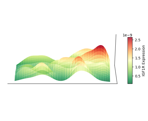
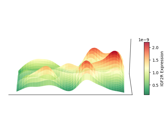
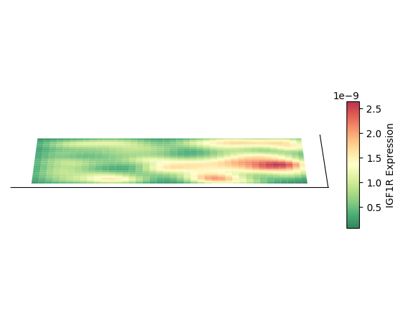
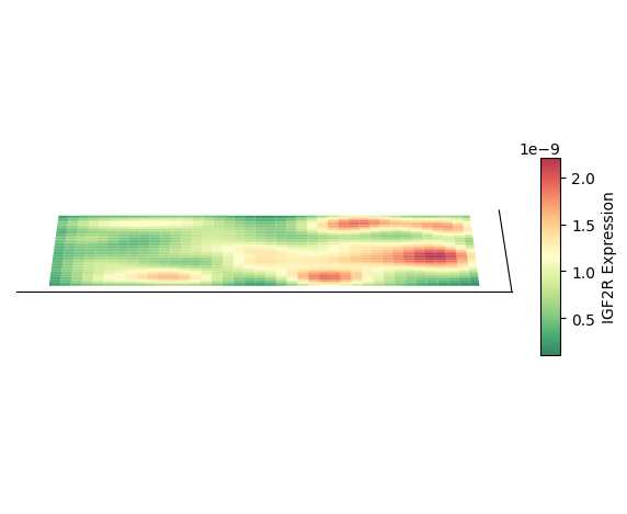
Plot 3D Spatial Density Map
Taking cell type AC as an example, plot its 3D spatial density map
python
for gene in ["IGF2","IGF1R","IGF2R"]:
        # Extract Coordinates and Gene Expression Values
        xy = merged_df[['x', 'y']].values.T  # Shape (2, N)
        expression = merged_df[gene].values  # Gene expression values

        # New: Check data point count and expression validity
        if xy.shape[1] <= 1 or np.all(np.isnan(expression)) or np.all(expression == 0):
            print(f"{sample} {gene} Insufficient data points or invalid expression values, skipping.")
            continue

        # Use gene expression values as weights for kernel density estimation
        # Note: Using expression values directly as z-axis height here
        kde_weights = gaussian_kde(xy, weights=expression, bw_method=0.2)

        # Create Grid
        xmin, xmax = merged_df.x.min(), merged_df.x.max()
        ymin, ymax = merged_df.y.min(), merged_df.y.max()
        xgrid = np.linspace(xmin, xmax, 200)
        ygrid = np.linspace(ymin, ymax, 200)
        X, Y = np.meshgrid(xgrid, ygrid)
        grid_points = np.vstack([X.ravel(), Y.ravel()])

        # Calculate weighted density (i.e., spatial distribution of gene expression)
        Z = kde_weights(grid_points).reshape(X.shape)

        # Create Canvas
        fig = plt.figure(figsize=(7, 5))
        ax3d = fig.add_subplot(111, projection='3d')

        # Set Aspect Ratio
        ax3d.set_box_aspect([15, 5, 5])

        # Cosmetic Settings
        ax3d.grid(False)
        ax3d.set_facecolor('white')
        ax3d.xaxis.set_pane_color((1.0, 1.0, 1.0, 1.0))
        ax3d.yaxis.set_pane_color((1.0, 1.0, 1.0, 1.0))
        ax3d.zaxis.set_pane_color((1.0, 1.0, 1.0, 1.0))

        # Hide Axes
        ax3d.set_xticks([])
        ax3d.set_yticks([])
        ax3d.set_zticks([])
        ax3d.set_xticklabels([])
        ax3d.set_yticklabels([])
        ax3d.set_xlabel('')
        ax3d.set_ylabel('')
        ax3d.set_zlabel('')

        # Plot Gene Expression Surface
        surf = ax3d.plot_surface(
            X, Y, Z,
            #cmap='viridis',          # Use heatmap color scheme for expression intensity
            cmap='RdYlGn_r',
            rstride=5,               # Row stride
            cstride=5,               # Column stride
            alpha=0.8,               # Appropriate transparency
            antialiased=True,
            edgecolor='none',
            linewidth=0.1
        )

        # Add color bar to indicate expression intensity
        cbar = fig.colorbar(surf, ax=ax3d, shrink=0.4, aspect=10, pad=0.05)
        cbar.set_label(f'{gene} Expression', fontsize=10)

        # Set View Angle (Top view from Y-axis)
        ax3d.view_init(elev=30, azim=-90)

        # Adjust Layout and Save
        plt.tight_layout()
        plt.subplots_adjust(left=0, right=0.95, top=0.95, bottom=0.05)
        #plt.savefig(f'{sample}_{gene}_expression3d.pdf')
        plt.show()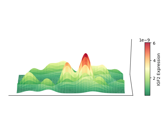
Plot 3D Spatial Density Mapping
Taking cell type AC as an example, plot its 3D spatial density mapping
python
for gene in ["IGF2","IGF1R","IGF2R"]:
        # Extract Coordinates and Gene Expression Values
        xy = merged_df[['x', 'y']].values.T  # Shape (2, N)
        expression = merged_df[gene].values  # Gene expression values

        # New: Check data point count and expression validity
        if xy.shape[1] <= 1 or np.all(np.isnan(expression)) or np.all(expression == 0):
            print(f"{sample} {gene} Insufficient data points or invalid expression values, skipping.")
            continue

        # Use gene expression values as weights for kernel density estimation
        # Note: Using expression values directly as z-axis height here
        kde_weights = gaussian_kde(xy, weights=expression, bw_method=0.2)

        # Create Grid
        xmin, xmax = merged_df.x.min(), merged_df.x.max()
        ymin, ymax = merged_df.y.min(), merged_df.y.max()
        xgrid = np.linspace(xmin, xmax, 200)
        ygrid = np.linspace(ymin, ymax, 200)
        X, Y = np.meshgrid(xgrid, ygrid)
        grid_points = np.vstack([X.ravel(), Y.ravel()])

        # Calculate weighted density (i.e., spatial distribution of gene expression)
        Z = kde_weights(grid_points).reshape(X.shape)

        # Create Canvas
        fig = plt.figure(figsize=(7, 5))
        ax3d = fig.add_subplot(111, projection='3d')

        # Set Aspect Ratio
        ax3d.set_box_aspect([15, 5, 0.01])

        # Cosmetic Settings
        ax3d.grid(False)
        ax3d.set_facecolor('white')
        ax3d.xaxis.set_pane_color((1.0, 1.0, 1.0, 1.0))
        ax3d.yaxis.set_pane_color((1.0, 1.0, 1.0, 1.0))
        ax3d.zaxis.set_pane_color((1.0, 1.0, 1.0, 1.0))

        # Hide Axes
        ax3d.set_xticks([])
        ax3d.set_yticks([])
        ax3d.set_zticks([])
        ax3d.set_xticklabels([])
        ax3d.set_yticklabels([])
        ax3d.set_xlabel('')
        ax3d.set_ylabel('')
        ax3d.set_zlabel('')

        # Plot Gene Expression Surface
        surf = ax3d.plot_surface(
            X, Y, Z,
            #cmap='viridis',          # Use heatmap color scheme for expression intensity
            cmap='RdYlGn_r',
            rstride=5,               # Row stride
            cstride=5,               # Column stride
            alpha=0.8,               # Appropriate transparency
            antialiased=True,
            edgecolor='none',
            linewidth=0.1
        )

        # Add color bar to indicate expression intensity
        cbar = fig.colorbar(surf, ax=ax3d, shrink=0.4, aspect=10, pad=0.05)
        cbar.set_label(f'{gene} Expression', fontsize=10)

        # Set View Angle (Top view from Y-axis)
        ax3d.view_init(elev=30, azim=-90)

        # Adjust Layout and Save
        plt.tight_layout()
        plt.subplots_adjust(left=0, right=0.95, top=0.95, bottom=0.05)
#        plt.savefig(f'{sample}_{gene}_expression2d.pdf')
        plt.show()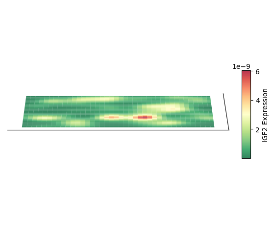
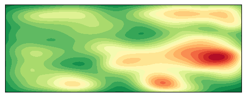
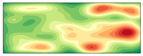
Plot 2D Density Map
python
for gene in ["IGF2","IGF1R","IGF2R"]:
        # Extract Coordinates and Gene Expression Values
        xy = merged_df[['x', 'y']].values.T  # Shape (2, N)
        expression = merged_df[gene].values  # Gene expression values

        # New: Check data point count and expression validity
        if xy.shape[1] <= 1 or np.all(np.isnan(expression)) or np.all(expression == 0):
            print(f"{sample} {gene} Insufficient data points or invalid expression values, skipping.")
            continue

        # Use gene expression values as weights for kernel density estimation
        # Note: Using expression values directly as z-axis height here
        kde_weights = gaussian_kde(xy, weights=expression, bw_method=0.2)

        # Create Grid
        xmin, xmax = merged_df.x.min(), merged_df.x.max()
        ymin, ymax = merged_df.y.min(), merged_df.y.max()
        xgrid = np.linspace(xmin, xmax, 200)
        ygrid = np.linspace(ymin, ymax, 200)
        X, Y = np.meshgrid(xgrid, ygrid)
        grid_points = np.vstack([X.ravel(), Y.ravel()])

        # Calculate weighted density (i.e., spatial distribution of gene expression)
        Z = kde_weights(grid_points).reshape(X.shape)

        fig2d, ax2d = plt.subplots(figsize=(6, 4))
        contour = ax2d.contourf(X, Y, Z, levels=20, cmap='RdYlGn_r')

        # Axis Settings
        ax2d.set(xlim=(xmin, xmax), ylim=(ymin, ymax), aspect='equal')

        # Remove Axis Ticks
        ax2d.set_xticks([])
        ax2d.set_yticks([])

        # Remove Axis Labels
        ax2d.set_xlabel('')
        ax2d.set_ylabel('')

        plt.show()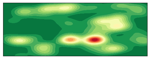
python