Seurat 单细胞转录组分析全流程教程 (QC / 整合 / 聚类)

作者: SeekGene

时长: 45 分钟

字数: 9.2k 字

更新: 2026-02-27

阅读: 0 次

3' 转录组 5' + 免疫组库 ATAC + RNA 双组学 FFPE 单细胞转录组 Notebooks 全序列转录组分析指南基础分析甲基化 + RNA 双组学空间转录组

Seurat 简介

Seurat 是一个功能全面的 R 包，专为单细胞 RNA 测序数据的质量控制、分析和探索而设计。由 Satija 实验室开发，Seurat 使用户能够：

物种支持：人和小鼠特异性基因模式。
质量控制和过滤：去除低质量细胞和基因。
DoubletFinder：自动双细胞检测和去除。
归一化和标准化：标准化跨细胞的表达数据。
降维：执行 PCA、t-SNE 和 UMAP 进行可视化。
多种整合方法：Harmony、CCA 和 merge。
细胞聚类：识别不同的细胞群体。
差异表达：查找每个簇的标记基因。

内核配置

重要提示：本教程应使用 "common_r" 内核运行。

所需包：

Seurat (>= 4.0)
DoubletFinder.
harmony (optional)
dplyr, ggplot2, patchwork.
RColorBrewer, viridis.

参数配置

配置所有分析参数，包括物种特异性设置和可视化颜色。

# === 分析参数说明 ===

# 数据路径 - 指定输入和输出目录
samples_parent_path <- "./data"  # 包含样本数据文件夹的目录
output_path <- "./result"     # 结果输出目录

# === 可视化参数 ===
# 绘图配色方案
DISCRETE_COLOR <- "Paired"     # 离散调色板: "Set1", "Set2", "Set3", "Dark2", "Paired", "Pastel1", "Pastel2", "Accent"
CONTINUOUS_COLOR <- "viridis" # 连续调色板: "viridis", "plasma", "inferno", "magma", "cividis"

# === 物种参数 ===
# 物种选择 - 影响过滤的基因模式 
species <- "human"  # 选项："human", "mouse" - 决定线粒体/核糖体/血红蛋白基因模式

# === 初始化参数 ===
# Seurat 对象创建期间的初始过滤
min_cells <- 3           # 表达某个基因的最小细胞数（过滤基因）
min_features_init <- 200 # 每个细胞的最小基因数（初始过滤）

# === 细胞质量过滤参数 ===
# 基于 RNA 特征和计数的二次过滤
min_features <- 100   # 每个细胞的最小基因数（最终过滤）
max_features <- 30000  # 每个细胞的最大基因数
min_count <- 300      # 每个细胞的最小总 RNA 计数
max_count <- 100000    # 每个细胞的最大总 RNA 计数

# === 物种特异性基因集过滤 ===
# 基于物种的自动基因模式检测
gene_set_filters <- list(
    mitochondrial = list(
        pattern = ifelse(species == "human", "^MT-", "^mt-"),  # 线粒体基因模式, Human: ^MT-, Mouse: ^mt-
        max_percent = 20,    # 每个细胞的最大线粒体基因百分比
        enabled = TRUE       # 启用/禁用此过滤器
    ),
    ribosomal = list(
        pattern = ifelse(species == "human", "^RP[SL]", "^Rp[sl]"),  # 核糖体基因模式, Human: ^RP[SL], Mouse: ^Rp[sl]
        min_percent = 3,    # 每个细胞的最小核糖体基因百分比
        enabled = FALSE      # 启用/禁用此过滤器
    ),
    hemoglobin = list(
        pattern = ifelse(species == "human", "^HB[^(P)]", "^Hb[^(p)]"),  # 血红蛋白基因模式, Human: ^HB[^(P)], Mouse: ^Hb[^(p)]
        max_percent = 5,     # 每个细胞的最大血红蛋白基因百分比
        enabled = FALSE      # CEnable/disable this filter
    )
)

# === 双细胞检测参数 ===
# 用于去除非自然双细胞的 DoubletFinder 设置
enable_doublet_detection <- TRUE  # 启用/禁用双细胞检测
expected_doublet_rate <- 0.075    # 预期双细胞率 (7.5% for 10K cells)
doublet_formation_rate <- 0.05    # pN 参数的人工双细胞形成率

# === 数据整合参数 ===
# 组合多个样本的方法
integration_method <- "Harmony"   # Options: "Harmony", "CCA", "merge"
selection_method <- "vst"         # 变异特征选择方法: "vst", "mean.var.plot", "dispersion"
nfeatures <- 2000                 # 要识别的高变异特征数量

# === 聚类参数 ===
# 基于图的聚类设置
clustering_resolution <- 0.5  # 聚类分辨率 (0.1-2.0, higher = more clusters)
dims_use <- 1:30              # 用于聚类和 UMAP 的主成分

# 创建输出目录
dir.create(output_path, recursive = TRUE, showWarnings = FALSE)

print("=== 分析参数已配置 ===")
print(paste("Samples parent directory:", samples_parent_path))
print(paste("Output directory:", output_path))
print(paste("Discrete color scheme:", DISCRETE_COLOR))
print(paste("Continuous color scheme:", CONTINUOUS_COLOR))
print(paste("Species:", species))
print(paste("DoubletFinder enabled:", enable_doublet_detection))
print(paste("Integration method:", integration_method))

output

[1] "=== ANALYSIS PARAMETERS CONFIGURED ==="
[1] "Samples parent directory: /home/demo-seekgene-com/workspace/project/demo-seekgene-com/Seurat/data"
[1] "Output directory: /home/demo-seekgene-com/workspace/project/demo-seekgene-com/Seurat/result"
[1] "Discrete color scheme: Paired"
[1] "Continuous color scheme: viridis"
[1] "Species: human"
[1] "DoubletFinder enabled: TRUE"
[1] "Integration method: Harmony"

Seurat 综合分析流程

本节提供了完整的 Seurat 工作流程的分步指南，从数据加载到标记基因查找。

加载库和数据

加载所有必需的库和样本数据。

# 加载核心库
library(Seurat)
library(dplyr)
library(patchwork)
library(ggplot2)
library(RColorBrewer)
library(viridis)

# 如果启用，加载 DoubletFinder
if (enable_doublet_detection) {
    tryCatch({
        library(DoubletFinder)
        print("✓ DoubletFinder loaded successfully")
    }, error = function(e) {
        print("⚠ Warning: DoubletFinder not available. Install with: devtools::install_github('chris-mcginnis-ucsf/DoubletFinder')")
        enable_doublet_detection <<- FALSE
    })
}

# 加载整合库
if (integration_method == "Harmony") {
    tryCatch({
        library(harmony)
        print("✓ Harmony loaded successfully")
    }, error = function(e) {
        print("⚠ Warning: Harmony not available. Switching to merge integration")
        integration_method <<- "merge"
    })
}

print(paste("Seurat version:", packageVersion("Seurat")))

output

Attaching SeuratObject

Attaching package: ‘dplyr’

The following objects are masked from ‘package:stats’:

filter, lag

The following objects are masked from ‘package:base’:

intersect, setdiff, setequal, union

Loading required package: viridisLite

[1] "✓ DoubletFinder loaded successfully"

Loading required package: Rcpp

[1] "✓ Harmony loaded successfully"
[1] "Seurat version: 4.4.0"

# 检测并加载样本数据
sample_dirs <- list.dirs(samples_parent_path, full.names = TRUE, recursive = FALSE)
sample_names <- basename(sample_dirs)
sample_dirs <- sample_dirs[!grepl("^\\.", sample_names)]
sample_names <- basename(sample_dirs)

print(paste("Found", length(sample_dirs), "sample directories:"))
for (i in 1:length(sample_names)) {
    print(paste("Sample", i, ":", sample_names[i]))
}

# 加载所有样本的数据
sample_data_list <- list()
successful_samples <- c()

for (i in 1:length(sample_dirs)) {
    sample_name <- sample_names[i]
    sample_path <- sample_dirs[i]
    
    tryCatch({
        sample_data <- Read10X(data.dir = sample_path)
        sample_data_list[[sample_name]] <- sample_data
        successful_samples <- c(successful_samples, sample_name)
        print(paste("✓ Successfully loaded", sample_name, ":", 
                   dim(sample_data)[1], "genes x", dim(sample_data)[2], "cells"))
    }, error = function(e) {
        print(paste("✗ Error loading", sample_name, ":", e$message))
    })
}

print(paste("Successfully loaded", length(successful_samples), "samples:", paste(successful_samples, collapse = ", ")))

output

[1] "Found 2 sample directories:"
[1] "Sample 1 : S133A"
[1] "Sample 2 : S133T"
[1] "✓ Successfully loaded S133A : 36601 genes x 6379 cells"
[1] "✓ Successfully loaded S133T : 36601 genes x 12220 cells"
[1] "Successfully loaded 2 samples: S133A, S133T"

创建 Seurat 对象并进行质控

创建 Seurat 对象并计算物种特异性 QC 指标。

# 创建 Seurat 对象
seurat_objects <- list()

for (sample_name in successful_samples) {
    seurat_obj <- CreateSeuratObject(
        counts = sample_data_list[[sample_name]], 
        project = sample_name, 
        min.cells = min_cells,
        min.features = min_features_init
    )
    
    seurat_obj$sample <- sample_name
    seurat_obj$species <- species
    
    # 计算物种特异性 QC 指标
    for (filter_name in names(gene_set_filters)) {
        filter_info <- gene_set_filters[[filter_name]]
        if (filter_info$enabled) {
            percent_col <- paste0("percent.", filter_name)
            seurat_obj[[percent_col]] <- PercentageFeatureSet(seurat_obj, pattern = filter_info$pattern)
            print(paste("✓ Calculated", filter_name, "for", sample_name, "using pattern:", filter_info$pattern))
        }
    }
    
    seurat_objects[[sample_name]] <- seurat_obj
}

# 合并样本
if (length(successful_samples) == 1) {
    combined_samples <- seurat_objects[[successful_samples[1]]]
} else {
    combined_samples <- merge(
        seurat_objects[[successful_samples[1]]], 
        y = seurat_objects[successful_samples[-1]], 
        add.cell.ids = successful_samples, 
        project = "Combined_Analysis"
    )
}

print(paste("Combined dataset:", ncol(combined_samples), "cells,", nrow(combined_samples), "genes"))
head(combined_samples@meta.data)

output

[1] "✓ Calculated mitochondrial for S133A using pattern: ^MT-"
[1] "✓ Calculated mitochondrial for S133T using pattern: ^MT-"
[1] "Combined dataset: 18518 cells, 24091 genes"

A data.frame: 6 × 6
	orig.ident	nCount_RNA	nFeature_RNA	sample	species	percent.mitochondrial
	<chr>	<dbl>	<int>	<chr>	<chr>	<dbl>
S133A_AAACCTGAGAGACTAT-1	S133A	2789	1097	S133A	human	5.4141269
S133A_AAACCTGAGCCGCCTA-1	S133A	2333	998	S133A	human	6.8152593
S133A_AAACCTGAGCCTCGTG-1	S133A	5630	1547	S133A	human	3.2149201
S133A_AAACCTGAGGGAGTAA-1	S133A	1230	572	S133A	human	17.3983740
S133A_AAACCTGAGGGTTCCC-1	S133A	1068	634	S133A	human	4.4007491
S133A_AAACCTGCACACCGCA-1	S133A	1940	701	S133A	human	0.7216495

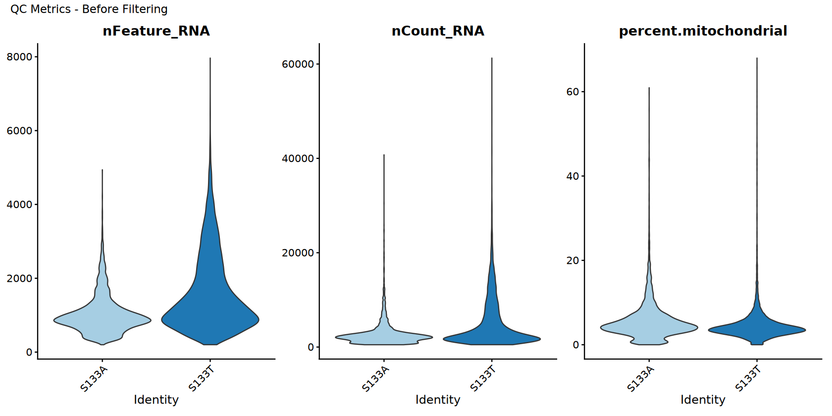
过滤前的质控可视化

在过滤前可视化质量控制指标。

# Set up colors
sample_colors <- brewer.pal(min(length(unique(combined_samples$sample)), 12), DISCRETE_COLOR)
if (length(unique(combined_samples$sample)) > 12) {
    sample_colors <- colorRampPalette(sample_colors)(length(unique(combined_samples$sample)))
}

# Store original data for comparison
combined_samples_original <- combined_samples
combined_samples_original$filter_status <- "Before Filtering"

# QC violin plots before filtering
options(repr.plot.width = 14, repr.plot.height = 7)
p_before <- VlnPlot(combined_samples_original, 
                     features = c("nFeature_RNA", "nCount_RNA", "percent.mitochondrial"), 
                     ncol = 3, 
                     cols = sample_colors,
                     pt.size = 0) + 
             plot_annotation(title = "QC Metrics - Before Filtering")

# Display plots
print(p_before)

# Save plots
ggsave(filename = file.path(output_path, "Step2_QC_before_filtering.pdf"), 
       plot = p_before, width = 15, height = 8)

print("QC visualization (before filtering) completed!")

output

Warning message in brewer.pal(min(length(unique(combined_samples$sample)), 12), :
“minimal value for n is 3, returning requested palette with 3 different levels
”

[1] "QC visualization (before filtering) completed!"

细胞过滤

Apply comprehensive filtering using robust methods.

# Store pre-filtering stats
pre_filter_cells <- ncol(combined_samples)

print("=== FILTERING ===")
print(paste("Starting with", pre_filter_cells, "cells"))

# Apply basic filters
filtered_samples <- combined_samples
filtered_samples <- subset(filtered_samples, subset = nFeature_RNA > min_features & nFeature_RNA < max_features)
filtered_samples <- subset(filtered_samples, subset = nCount_RNA > min_count & nCount_RNA < max_count)

# Apply species-specific gene set filters
for (filter_name in names(gene_set_filters)) {
    filter_info <- gene_set_filters[[filter_name]]
    if (filter_info$enabled) {
        percent_col <- paste0("percent.", filter_name)
        if (percent_col %in% colnames(filtered_samples@meta.data)) {
            cells_before <- ncol(filtered_samples)
            
            # Use metadata filtering for robustness
            meta_data <- filtered_samples@meta.data
            
            # 检查是最大值过滤还是最小值过滤
            if ("max_percent" %in% names(filter_info)) {
                keep_cells <- meta_data[[percent_col]] < filter_info$max_percent
                filter_type <- paste("< ", filter_info$max_percent, "%")
            } else if ("min_percent" %in% names(filter_info)) {
                keep_cells <- meta_data[[percent_col]] > filter_info$min_percent
                filter_type <- paste("> ", filter_info$min_percent, "%")
            }
            
            cell_names_to_keep <- rownames(meta_data)[keep_cells]
            filtered_samples <- subset(filtered_samples, cells = cell_names_to_keep)
            
            cells_after <- ncol(filtered_samples)
            print(paste("✓", filter_name, "filter (", filter_type, "):", 
                      cells_before, "→", cells_after, "cells"))
        }
    }
}

combined_samples <- filtered_samples
post_filter_cells <- ncol(combined_samples)

print(paste("Cells after filtering:", post_filter_cells))
print(paste("Cells retained:", round((post_filter_cells/pre_filter_cells)*100, 2), "%"))

output

[1] "=== FILTERING ==="
[1] "Starting with 18518 cells"
[1] "✓ mitochondrial filter ( < 20 % ): 18518 → 18296 cells"
[1] "Cells after filtering: 18296"
[1] "Cells retained: 98.8 %"
[1] "Starting with 18518 cells"
[1] "✓ mitochondrial filter (< 20 %): 18443 → 18224 cells"
[1] "Cells after filtering: 18224"
[1] "Cells retained: 98.41 %"

QC Visualization After Filtering

Visualize quality control metrics after filtering and compare with before.

# Add filter status to the filtered data
combined_samples$filter_status <- "After Filtering"

# QC violin plots after filtering
options(repr.plot.width = 14, repr.plot.height = 7)
p_after <- VlnPlot(combined_samples, 
                    features = c("nFeature_RNA", "nCount_RNA", "percent.mitochondrial"), 
                    ncol = 3, 
                    cols = sample_colors,
                    pt.size = 0) + 
            plot_annotation(title = "QC Metrics - After Filtering")

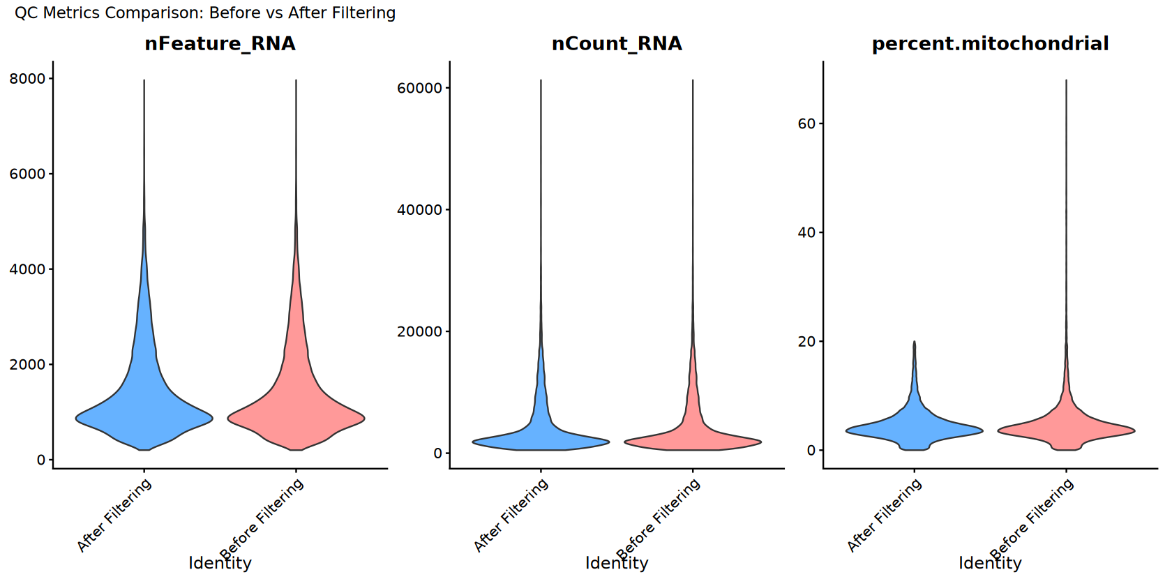
# Create combined comparison plots
# Combine datasets for comparison
combined_for_comparison <- merge(combined_samples_original, combined_samples, 
                                add.cell.ids = c("before", "after"))

# Comparison violin plot
comparison_colors <- c("Before Filtering" = "#FF9999", "After Filtering" = "#66B2FF")
p_comparison <- VlnPlot(combined_for_comparison, 
                       features = c("nFeature_RNA", "nCount_RNA", "percent.mitochondrial"), 
                       ncol = 3, 
                       group.by = "filter_status",
                       cols = comparison_colors,
                       pt.size = 0) + 
               plot_annotation(title = "QC Metrics Comparison: Before vs After Filtering")

# Display plots
print(p_after)
print(p_comparison)

# Save plots
ggsave(filename = file.path(output_path, "Step3_QC_after_filtering.pdf"), 
       plot = p_after, width = 15, height = 8)
ggsave(filename = file.path(output_path, "Step3_QC_comparison_before_after.pdf"), 
       plot = p_comparison, width = 15, height = 8)

print("QC visualization (after filtering and comparison) completed!")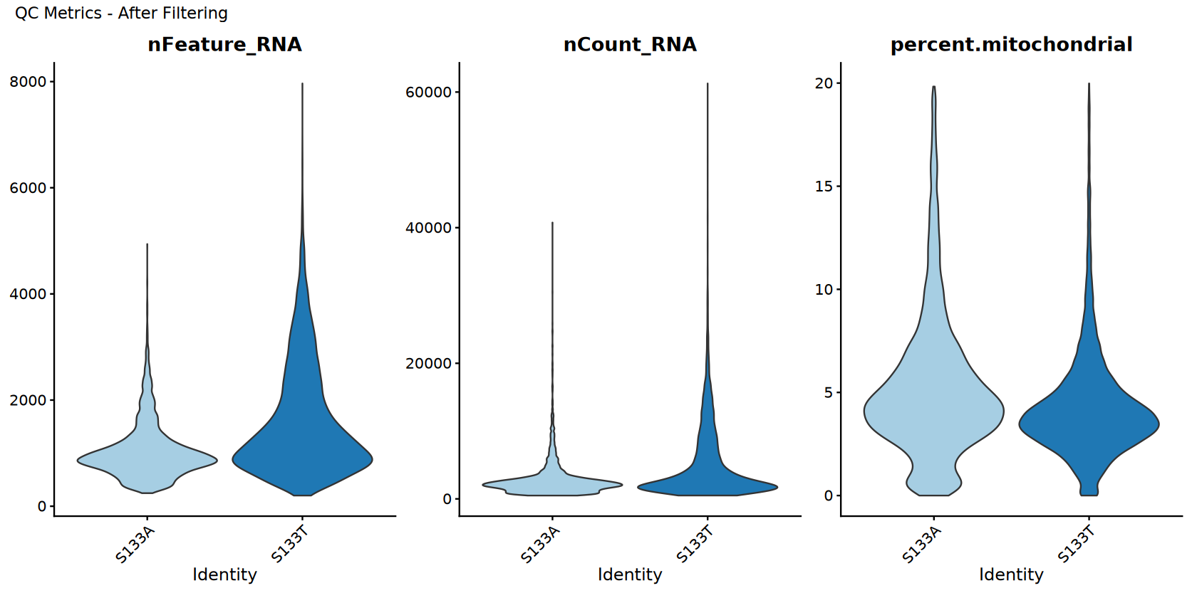

[1] "QC visualization (after filtering and comparison) completed!"

DoubletFinder 分析

Use DoubletFinder to identify and remove doublets.

if (enable_doublet_detection) {
    print("=== DOUBLET DETECTION WITH DOUBLETFINDER ===")
    
    # Record cell count before doublet detection
    pre_doublet_cells <- ncol(combined_samples)
    
    # Prepare data for DoubletFinder (required preprocessing)
    combined_samples <- NormalizeData(combined_samples)
    combined_samples <- FindVariableFeatures(combined_samples, selection.method = selection_method, nfeatures = nfeatures)
    combined_samples <- ScaleData(combined_samples)
    combined_samples <- RunPCA(combined_samples)
    
    # Parameter sweep to find optimal pK value
    print("Running parameter sweep to optimize pK...")
    sweep.res.list <- paramSweep(seu = combined_samples,
                                PCs = 1:10, 
                                sct = FALSE)
    sweep.stats <- summarizeSweep(sweep.res.list, GT = FALSE)
    bcmvn <- find.pK(sweep.stats)
    optimal_pk <- as.numeric(as.character(bcmvn$pK[which.max(bcmvn$BCmetric)]))
    
    print(paste("Optimal pK found:", optimal_pk))
    
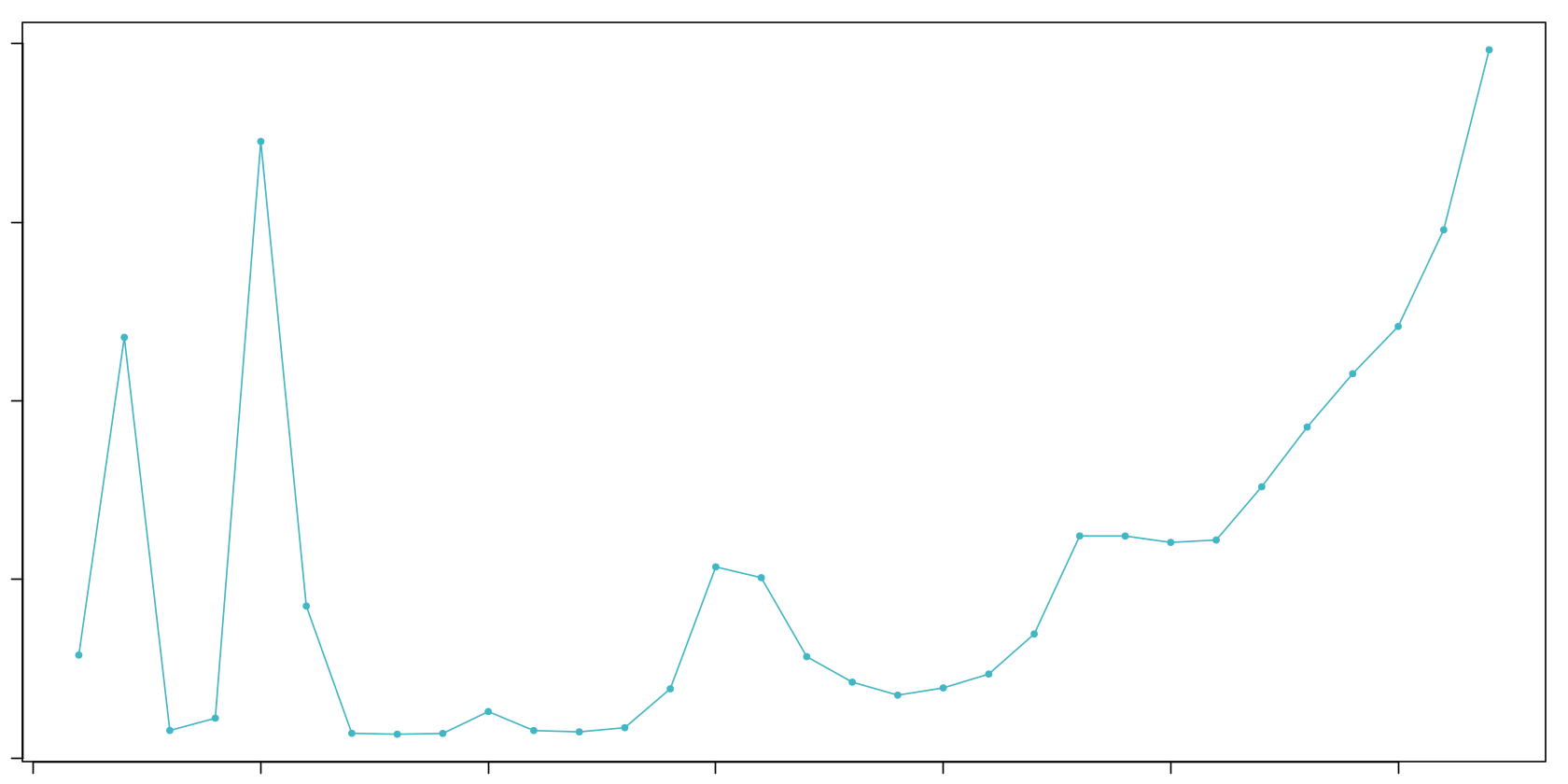
    # Visualize pK optimization
    pk_plot <- ggplot(bcmvn, aes(x = pK, y = BCmetric)) +
              geom_point() +
              geom_line() +
              geom_vline(xintercept = optimal_pk, color = "red", linetype = "dashed") +
              ggtitle(paste("pK Optimization (Optimal pK =", optimal_pk, ")")) +
              theme_minimal()
    
    ggsave(filename = file.path(output_path, "Step4_DoubletFinder_pK_optimization.pdf"), 
           plot = pk_plot, width = 8, height = 6)
    
    # Calculate expected number of doublets
    nExp_poi.adj <- round(expected_doublet_rate * pre_doublet_cells)
    print(paste("Expected number of doublets:", nExp_poi.adj))
    
    # Run DoubletFinder with optimized parameters
    print("Running DoubletFinder doublet detection...")
    combined_samples <- doubletFinder(seu = combined_samples,
                                     PCs = 1:10,
                                     pN = doublet_formation_rate,
                                     pK = optimal_pk,
                                     nExp = nExp_poi.adj,
                                     reuse.pANN = FALSE,
                                     sct = FALSE)
    
    # Find doublet classification columns in metadata
    doublet_cols <- grep("DF.classifications", colnames(combined_samples@meta.data), value = TRUE)
    pann_cols <- grep("pANN", colnames(combined_samples@meta.data), value = TRUE)
    
    if (length(doublet_cols) > 0) {
        doublet_col <- doublet_cols[1]
        pann_col <- pann_cols[1]
        
        print(paste("Found doublet classification column:", doublet_col))
        print(paste("Found pANN score column:", pann_col))
        
        # Display doublet detection results
        doublet_counts <- table(combined_samples@meta.data[[doublet_col]])
        print("Doublet detection results:")
        print(doublet_counts)
        
        # Create UMAP for doublet visualization
        combined_samples <- RunUMAP(combined_samples, dims = dims_use)
        
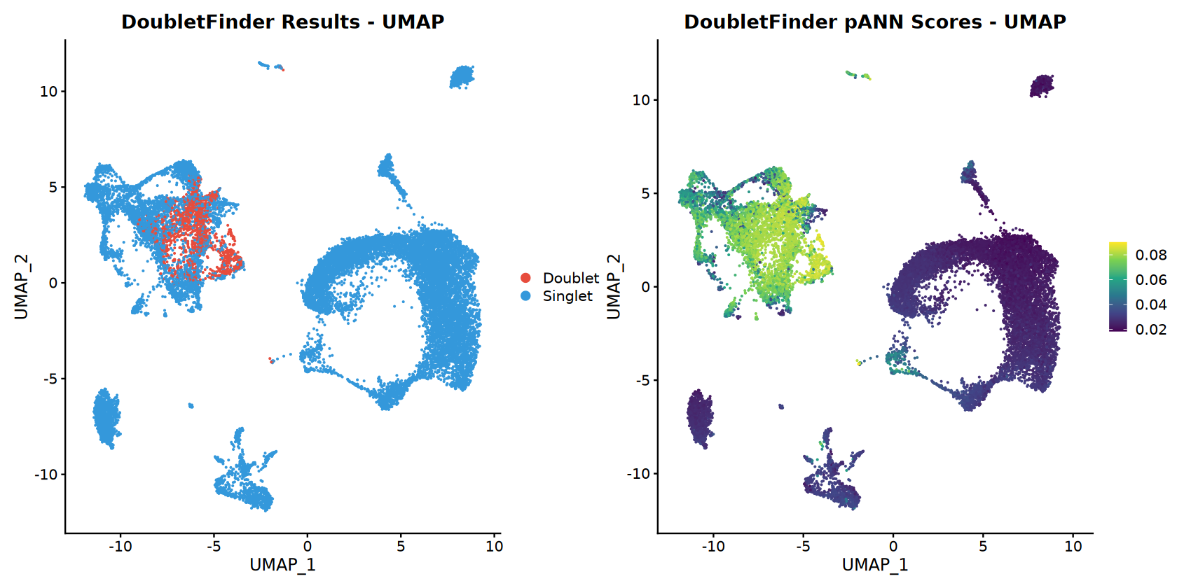
        # Doublet classification UMAP
        doublet_colors <- c("Singlet" = "#3498db", "Doublet" = "#e74c3c")
        p_doublet_umap <- DimPlot(combined_samples, 
                                 reduction = "umap", 
                                 group.by = doublet_col,
                                 cols = doublet_colors) +
                         ggtitle("DoubletFinder Results - UMAP")
        
        # pANN score UMAP (continuous)
        p_pann_umap <- FeaturePlot(combined_samples, 
                                  features = pann_col,
                                  reduction = "umap") +
                      scale_color_viridis_c(option = CONTINUOUS_COLOR) +
                      ggtitle("DoubletFinder pANN Scores - UMAP")
        
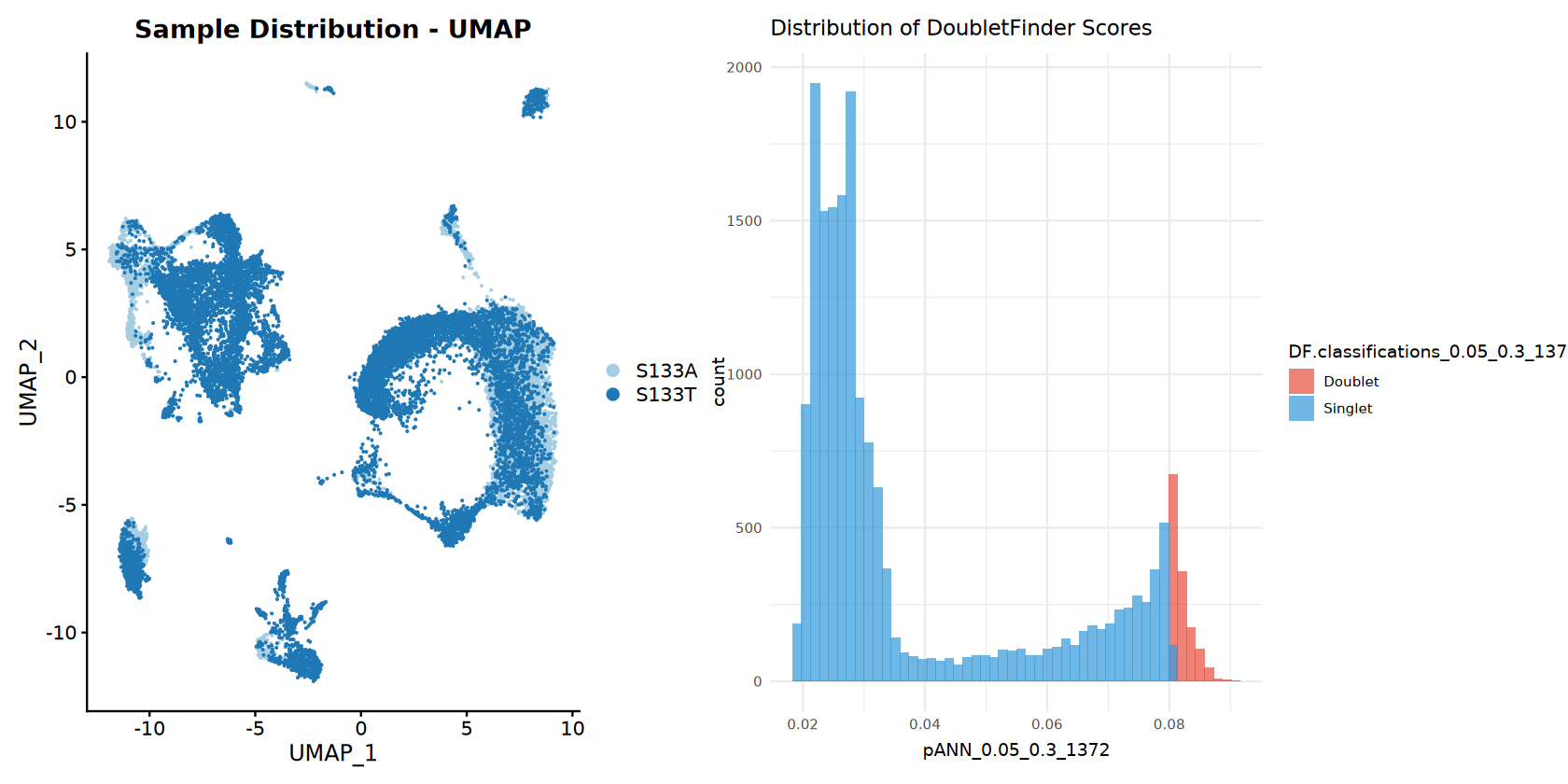
        # Sample distribution UMAP
        p_sample_umap <- DimPlot(combined_samples, 
                                reduction = "umap", 
                                group.by = "sample",
                                cols = sample_colors) +
                        ggtitle("Sample Distribution - UMAP")
        
        # Doublet score distribution
        p_pann_hist <- ggplot(combined_samples@meta.data, aes_string(x = pann_col, fill = doublet_col)) +
                      geom_histogram(bins = 50, alpha = 0.7, position = "identity") +
                      scale_fill_manual(values = doublet_colors) +
                      ggtitle("Distribution of DoubletFinder Scores") +
                      theme_minimal()
        
        # Display doublet plots
        print(p_doublet_umap + p_pann_umap)
        print(p_sample_umap + p_pann_hist)
        
        # Save doublet plots
        ggsave(filename = file.path(output_path, "Step4_DoubletFinder_UMAP_classification.pdf"), 
               plot = p_doublet_umap + p_pann_umap, width = 12, height = 6)
        ggsave(filename = file.path(output_path, "Step4_DoubletFinder_sample_and_scores.pdf"), 
               plot = p_sample_umap + p_pann_hist, width = 12, height = 6)
        
        # Remove doublets by filtering to keep only singlets
        meta_data <- combined_samples@meta.data
        singlet_cells <- rownames(meta_data)[meta_data[[doublet_col]] == "Singlet"]
        combined_samples <- subset(combined_samples, cells = singlet_cells)
        
        # Calculate and report doublet removal statistics
        post_doublet_cells <- ncol(combined_samples)
        doublets_removed <- pre_doublet_cells - post_doublet_cells
        
        print(paste("Doublets removed:", doublets_removed, "(", 
                   round((doublets_removed/pre_doublet_cells)*100, 2), "% of cells)"))
        print(paste("Remaining cells:", post_doublet_cells))
        
    } else {
        print("Warning: Could not find doublet classification column in metadata")
    }
    
} else {
    print("=== DOUBLET DETECTION SKIPPED ===")
    # Still run basic preprocessing
    combined_samples <- NormalizeData(combined_samples)
    combined_samples <- FindVariableFeatures(combined_samples, selection.method = selection_method, nfeatures = nfeatures)
    combined_samples <- ScaleData(combined_samples)
    combined_samples <- RunPCA(combined_samples)
}

print("DoubletFinder analysis completed!")

output

[1] "=== DOUBLET DETECTION WITH DOUBLETFINDER ==="

Centering and scaling data matrix

PC_ 1
Positive: IFI30, CST3, CD68, LYZ, CTSB, C1QA, C1QC, FCGR2A, MS4A6A, C1QB
MS4A7, TMEM176B, HLA-DQB1, TMEM176A, GSN, CTSZ, CD14, MAFB, C15orf48, IGSF6
IER3, SERPINA1, CYBB, SLC8A1, ALCAM, CXCL2, CXCL8, PLAUR, TGFBI, TNFSF13
Negative: GZMA, KLRB1, NKG7, GZMH, GZMB, FKBP11, ODC1, TNFRSF18, IFNG, CTSW
LAIR2, GZMK, GNLY, CD8A, PRF1, FOXP3, MZB1, HOPX, TNFRSF4, KLRD1
IL12RB2, HPGD, CD79A, C12orf75, LINC01943, SPON2, KLRC1, XCL1, MAGEH1, CD40LG
PC_ 2
Positive: DCN, COL6A2, RARRES2, COL1A2, C1S, LUM, COL6A1, SFRP2, C1R, FSTL1
MMP2, SPARC, ISLR, FBLN1, AEBP1, CTSK, NNMT, CCN1, CALD1, SERPING1
FBLN2, COL6A3, FBN1, CCDC80, PCOLCE, MFAP4, COL12A1, IGFBP7, SPARCL1, COL1A1
Negative: IL1B, BCL2A1, LYZ, CXCL8, OLR1, SERPINA1, G0S2, IFI30, PLAUR, HLA-DQB1
CCL3L1, KYNU, MS4A6A, EREG, C15orf48, FCN1, RNF144B, SLC8A1, NLRP3, CCL3
CLEC10A, C5AR1, IL1RN, CD86, CALHM6, CSF2RA, S100A9, MCTP1, TREM1, MS4A7
PC_ 3
Positive: THBS1, AQP9, EREG, FCN1, NLRP3, VCAN, S100A8, CD300E, C5AR1, DENND5A
S100A9, MIR3945HG, SLC11A1, IL1B, OLR1, TREM1, LUCAT1, CXCL8, CXCL2, PLAUR
RNF144B, CXCL3, S100A12, AC015912.3, BCL2A1, PTGS2, MAP4K4, TNFAIP6, MCEMP1, SESTD1
Negative: UBE2C, PCLAF, TYMS, MKI67, BIRC5, S100B, STMN1, CD1A, RRM2, AURKB
TOP2A, GTSE1, ZWINT, TK1, CCNA2, IL22RA2, CKS1B, CDC20, CENPF, HLA-DQB2
TPX2, CDCA3, TUBA1B, PKIB, CDK1, TUBB, C1QB, TROAP, CCNB2, C1QC
PC_ 4
Positive: APOE, RNASE1, APOC1, DERL3, MZB1, IGHG1, FOLR2, SLCO2B1, SELENOP, MERTK
LGMN, GPNMB, TREM2, PRDX4, SLC40A1, DAB2, PLTP, PLD3, STAB1, IGKC
A2M, CD9, IGHG3, IGHG2, TNFRSF17, CD79A, POU2AF1, KCNMA1, JCHAIN, C2
Negative: UBE2C, BCL2A1, TYMS, IL1B, MKI67, BIRC5, PCLAF, EREG, THBS1, RRM2
NLRP3, FCN1, GTSE1, AURKB, CFP, TOP2A, AQP9, CD1A, CD1E, CD1C
CCNA2, S100A8, CSTA, BASP1, MIR3945HG, CDCA3, G0S2, HMGB2, IL1R2, CDK1
PC_ 5
Positive: DERL3, MZB1, IGHG1, IGKC, CD79A, POU2AF1, IGHG3, SDC1, JCHAIN, TNFRSF17
IGHG2, AC012236.1, PRDX4, IGLC2, FKBP11, JSRP1, TXNDC5, IGLV3-1, FCRL5, SSR4
DPEP1, SPAG4, SEC11C, XBP1, IGLC3, FAM92B, IGHJ4, IGLV6-57, AF127936.2, LINC02362
Negative: TPSAB1, CPA3, TPSB2, TPSD1, KIT, MS4A2, GATA2, HPGDS, SLC24A3, CLU
VWA5A, RHEX, IL1RL1, AL157895.1, FER, SLC18A2, LTC4S, RGS13, HDC, ENPP3
NSMCE1, HPGD, CD9, ADAM12, CADPS, CAVIN2, ITGA9, TIMP3, BNC2, RHOBTB3

[1] "Running parameter sweep to optimize pK..."

Loading required package: fields

Loading required package: spam

Spam version 2.11-1 (2025-01-20) is loaded.
Type 'help( Spam)' or 'demo( spam)' for a short introduction
and overview of this package.
Help for individual functions is also obtained by adding the
suffix '.spam' to the function name, e.g. 'help( chol.spam)'.

Attaching package: ‘spam’

The following objects are masked from ‘package:base’:

backsolve, forwardsolve

Try help(fields) to get started.

Loading required package: parallel

[1] "Creating artificial doublets for pN = 5%"
[1] "Creating Seurat object..."
[1] "Normalizing Seurat object..."
[1] "Finding variable genes..."
[1] "Scaling data..."

Centering and scaling data matrix

[1] "Running PCA..."
[1] "Calculating PC distance matrix..."
[1] "Defining neighborhoods..."
[1] "Computing pANN across all pK..."
[1] "pK = 0.001..."
[1] "pK = 0.005..."
[1] "pK = 0.01..."
[1] "pK = 0.02..."
[1] "pK = 0.03..."
[1] "pK = 0.04..."
[1] "pK = 0.05..."
[1] "pK = 0.06..."
[1] "pK = 0.07..."
[1] "pK = 0.08..."
[1] "pK = 0.09..."
[1] "pK = 0.1..."
[1] "pK = 0.11..."
[1] "pK = 0.12..."
[1] "pK = 0.13..."
[1] "pK = 0.14..."
[1] "pK = 0.15..."
[1] "pK = 0.16..."
[1] "pK = 0.17..."
[1] "pK = 0.18..."
[1] "pK = 0.19..."
[1] "pK = 0.2..."
[1] "pK = 0.21..."
[1] "pK = 0.22..."
[1] "pK = 0.23..."
[1] "pK = 0.24..."
[1] "pK = 0.25..."
[1] "pK = 0.26..."
[1] "pK = 0.27..."
[1] "pK = 0.28..."
[1] "pK = 0.29..."
[1] "pK = 0.3..."
[1] "Creating artificial doublets for pN = 10%"
[1] "Creating Seurat object..."
[1] "Normalizing Seurat object..."
[1] "Finding variable genes..."
[1] "Scaling data..."

Centering and scaling data matrix

[1] "Running PCA..."
[1] "Calculating PC distance matrix..."
[1] "Defining neighborhoods..."
[1] "Computing pANN across all pK..."
[1] "pK = 0.001..."
[1] "pK = 0.005..."
[1] "pK = 0.01..."
[1] "pK = 0.02..."
[1] "pK = 0.03..."
[1] "pK = 0.04..."
[1] "pK = 0.05..."
[1] "pK = 0.06..."
[1] "pK = 0.07..."
[1] "pK = 0.08..."
[1] "pK = 0.09..."
[1] "pK = 0.1..."
[1] "pK = 0.11..."
[1] "pK = 0.12..."
[1] "pK = 0.13..."
[1] "pK = 0.14..."
[1] "pK = 0.15..."
[1] "pK = 0.16..."
[1] "pK = 0.17..."
[1] "pK = 0.18..."
[1] "pK = 0.19..."
[1] "pK = 0.2..."
[1] "pK = 0.21..."
[1] "pK = 0.22..."
[1] "pK = 0.23..."
[1] "pK = 0.24..."
[1] "pK = 0.25..."
[1] "pK = 0.26..."
[1] "pK = 0.27..."
[1] "pK = 0.28..."
[1] "pK = 0.29..."
[1] "pK = 0.3..."
[1] "Creating artificial doublets for pN = 15%"
[1] "Creating Seurat object..."
[1] "Normalizing Seurat object..."
[1] "Finding variable genes..."
[1] "Scaling data..."

Centering and scaling data matrix

[1] "Running PCA..."
[1] "Calculating PC distance matrix..."
[1] "Defining neighborhoods..."
[1] "Computing pANN across all pK..."
[1] "pK = 0.001..."
[1] "pK = 0.005..."
[1] "pK = 0.01..."
[1] "pK = 0.02..."
[1] "pK = 0.03..."
[1] "pK = 0.04..."
[1] "pK = 0.05..."
[1] "pK = 0.06..."
[1] "pK = 0.07..."
[1] "pK = 0.08..."
[1] "pK = 0.09..."
[1] "pK = 0.1..."
[1] "pK = 0.11..."
[1] "pK = 0.12..."
[1] "pK = 0.13..."
[1] "pK = 0.14..."
[1] "pK = 0.15..."
[1] "pK = 0.16..."
[1] "pK = 0.17..."
[1] "pK = 0.18..."
[1] "pK = 0.19..."
[1] "pK = 0.2..."
[1] "pK = 0.21..."
[1] "pK = 0.22..."
[1] "pK = 0.23..."
[1] "pK = 0.24..."
[1] "pK = 0.25..."
[1] "pK = 0.26..."
[1] "pK = 0.27..."
[1] "pK = 0.28..."
[1] "pK = 0.29..."
[1] "pK = 0.3..."
[1] "Creating artificial doublets for pN = 20%"
[1] "Creating Seurat object..."
[1] "Normalizing Seurat object..."
[1] "Finding variable genes..."
[1] "Scaling data..."

Centering and scaling data matrix

[1] "Running PCA..."
[1] "Calculating PC distance matrix..."
[1] "Defining neighborhoods..."
[1] "Computing pANN across all pK..."
[1] "pK = 0.001..."
[1] "pK = 0.005..."
[1] "pK = 0.01..."
[1] "pK = 0.02..."
[1] "pK = 0.03..."
[1] "pK = 0.04..."
[1] "pK = 0.05..."
[1] "pK = 0.06..."
[1] "pK = 0.07..."
[1] "pK = 0.08..."
[1] "pK = 0.09..."
[1] "pK = 0.1..."
[1] "pK = 0.11..."
[1] "pK = 0.12..."
[1] "pK = 0.13..."
[1] "pK = 0.14..."
[1] "pK = 0.15..."
[1] "pK = 0.16..."
[1] "pK = 0.17..."
[1] "pK = 0.18..."
[1] "pK = 0.19..."
[1] "pK = 0.2..."
[1] "pK = 0.21..."
[1] "pK = 0.22..."
[1] "pK = 0.23..."
[1] "pK = 0.24..."
[1] "pK = 0.25..."
[1] "pK = 0.26..."
[1] "pK = 0.27..."
[1] "pK = 0.28..."
[1] "pK = 0.29..."
[1] "pK = 0.3..."
[1] "Creating artificial doublets for pN = 25%"
[1] "Creating Seurat object..."
[1] "Normalizing Seurat object..."
[1] "Finding variable genes..."
[1] "Scaling data..."

Centering and scaling data matrix

[1] "Running PCA..."
[1] "Calculating PC distance matrix..."
[1] "Defining neighborhoods..."
[1] "Computing pANN across all pK..."
[1] "pK = 0.001..."
[1] "pK = 0.005..."
[1] "pK = 0.01..."
[1] "pK = 0.02..."
[1] "pK = 0.03..."
[1] "pK = 0.04..."
[1] "pK = 0.05..."
[1] "pK = 0.06..."
[1] "pK = 0.07..."
[1] "pK = 0.08..."
[1] "pK = 0.09..."
[1] "pK = 0.1..."
[1] "pK = 0.11..."
[1] "pK = 0.12..."
[1] "pK = 0.13..."
[1] "pK = 0.14..."
[1] "pK = 0.15..."
[1] "pK = 0.16..."
[1] "pK = 0.17..."
[1] "pK = 0.18..."
[1] "pK = 0.19..."
[1] "pK = 0.2..."
[1] "pK = 0.21..."
[1] "pK = 0.22..."
[1] "pK = 0.23..."
[1] "pK = 0.24..."
[1] "pK = 0.25..."
[1] "pK = 0.26..."
[1] "pK = 0.27..."
[1] "pK = 0.28..."
[1] "pK = 0.29..."
[1] "pK = 0.3..."
[1] "Creating artificial doublets for pN = 30%"
[1] "Creating Seurat object..."
[1] "Normalizing Seurat object..."
[1] "Finding variable genes..."
[1] "Scaling data..."

Centering and scaling data matrix

[1] "Running PCA..."
[1] "Calculating PC distance matrix..."
[1] "Defining neighborhoods..."
[1] "Computing pANN across all pK..."
[1] "pK = 0.001..."
[1] "pK = 0.005..."
[1] "pK = 0.01..."
[1] "pK = 0.02..."
[1] "pK = 0.03..."
[1] "pK = 0.04..."
[1] "pK = 0.05..."
[1] "pK = 0.06..."
[1] "pK = 0.07..."
[1] "pK = 0.08..."
[1] "pK = 0.09..."
[1] "pK = 0.1..."
[1] "pK = 0.11..."
[1] "pK = 0.12..."
[1] "pK = 0.13..."
[1] "pK = 0.14..."
[1] "pK = 0.15..."
[1] "pK = 0.16..."
[1] "pK = 0.17..."
[1] "pK = 0.18..."
[1] "pK = 0.19..."
[1] "pK = 0.2..."
[1] "pK = 0.21..."
[1] "pK = 0.22..."
[1] "pK = 0.23..."
[1] "pK = 0.24..."
[1] "pK = 0.25..."
[1] "pK = 0.26..."
[1] "pK = 0.27..."
[1] "pK = 0.28..."
[1] "pK = 0.29..."
[1] "pK = 0.3..."

Loading required package: KernSmooth

KernSmooth 2.23 loaded
Copyright M. P. Wand 1997-2009

Loading required package: ROCR

NULL
[1] "Optimal pK found: 0.3"

\`geom_line()\`: Each group consists of only one observation.
ℹ Do you need to adjust the group aesthetic?

[1] "Expected number of doublets: 1372"
[1] "Running DoubletFinder doublet detection..."
[1] "Creating 963 artificial doublets..."
[1] "Creating Seurat object..."
[1] "Normalizing Seurat object..."
[1] "Finding variable genes..."
[1] "Scaling data..."

Centering and scaling data matrix

[1] "Running PCA..."
[1] "Calculating PC distance matrix..."
[1] "Computing pANN..."
[1] "Classifying doublets.."
[1] "Found doublet classification column: DF.classifications_0.05_0.3_1372"
[1] "Found pANN score column: pANN_0.05_0.3_1372"
[1] "Doublet detection results:"

Doublet Singlet
1372 16924

Warning message:
“The default method for RunUMAP has changed from calling Python UMAP via reticulate to the R-native UWOT using the cosine metric
To use Python UMAP via reticulate, set umap.method to 'umap-learn' and metric to 'correlation'
This message will be shown once per session”
15:43:13 UMAP embedding parameters a = 0.9922 b = 1.112

15:43:13 Read 18296 rows and found 30 numeric columns

15:43:13 Using Annoy for neighbor search, n_neighbors = 30

15:43:13 Building Annoy index with metric = cosine, n_trees = 50

0% 10 20 30 40 50 60 70 80 90 100%

[----|----|----|----|----|----|----|----|----|----|

*
*
*
*
*
*
*
*
*
*
*
*
*
*
*
*
*
*
*
*
*
*
*
*
*
*
*
*
*
*
*
*
*
*
*
*
*
*
*
*
*
*
*
*
*
*
*
*
*
*
|

15:43:15 Writing NN index file to temp file /tmp/RtmpdByI5A/file22c7390f61b

15:43:15 Searching Annoy index using 1 thread, search_k = 3000

15:43:21 Annoy recall = 100%

15:43:21 Commencing smooth kNN distance calibration using 1 thread
with target n_neighbors = 30

15:43:22 Initializing from normalized Laplacian + noise (using irlba)

15:43:24 Commencing optimization for 200 epochs, with 826488 positive edges

15:43:24 Using rng type: pcg

15:43:33 Optimization finished

Scale for colour is already present.
Adding another scale for colour, which will replace the existing scale.
Warning message:
“\`aes_string()\` was deprecated in ggplot2 3.0.0.
ℹ Please use tidy evaluation idioms with \`aes()\`.
ℹ See also \`vignette("ggplot2-in-packages")\` for more information.”

[1] "Doublets removed: 1372 ( 7.5 % of cells)"
[1] "Remaining cells: 16924"
[1] "DoubletFinder analysis completed!"

数据整合

Integrate samples using Harmony, CCA, or merge.

if (length(successful_samples) > 1) {
    print(paste("Multiple samples detected. Using", integration_method, "integration"))
    
    if (integration_method == "Harmony") {
        # Harmony integration
        combined_samples <- RunHarmony(combined_samples, group.by.vars = "sample")
        reduction_use <- "harmony"
        print("✓ Harmony integration completed")
        
    } else if (integration_method == "CCA") {
        # CCA integration
        sample_list <- SplitObject(combined_samples, split.by = "sample")
        
        sample_list <- lapply(sample_list, function(x) {
            x <- NormalizeData(x)
            x <- FindVariableFeatures(x, selection.method = selection_method, nfeatures = nfeatures)
        })
        
        features <- SelectIntegrationFeatures(object.list = sample_list, nfeatures = nfeatures)
        anchors <- FindIntegrationAnchors(object.list = sample_list, anchor.features = features)
        combined_samples <- IntegrateData(anchorset = anchors)
        
        DefaultAssay(combined_samples) <- "integrated"
        combined_samples <- ScaleData(combined_samples, verbose = FALSE)
        combined_samples <- RunPCA(combined_samples, npcs = 30, verbose = FALSE)
        
        reduction_use <- "pca"
        print("✓ CCA integration completed")
        
    } else if (integration_method == "merge") {
        # Simple merge (no batch correction)
        reduction_use <- "pca"
        print("✓ Simple merge completed (no batch correction)")
    }
} else {
    reduction_use <- "pca"
    print("Single sample - no integration needed")
}

print(paste("Reduction method for clustering:", reduction_use))

output

[1] "Multiple samples detected. Using Harmony integration"

Transposing data matrix

Initializing state using k-means centroids initialization

Harmony 1/10

Harmony 2/10

Harmony 3/10

Harmony 4/10

Harmony converged after 4 iterations

Warning message:
“Invalid name supplied, making object name syntactically valid. New object name is Seurat..ProjectDim.RNA.harmony; see ?make.names for more details on syntax validity”

[1] "✓ Harmony integration completed"
[1] "Reduction method for clustering: harmony"

聚类分析

Perform graph-based clustering.

# Clustering
combined_samples <- FindNeighbors(combined_samples, reduction = reduction_use, dims = dims_use)
combined_samples <- FindClusters(combined_samples, resolution = clustering_resolution)

# UMAP visualization
combined_samples <- RunUMAP(combined_samples, reduction = reduction_use, dims = dims_use)

print("=== CLUSTERING RESULTS ===")
print(paste("Integration method:", integration_method))
print(paste("Resolution:", clustering_resolution))
print(paste("Number of clusters:", length(unique(Idents(combined_samples)))))

cluster_sizes <- table(Idents(combined_samples))
print("Cluster sizes:")
print(cluster_sizes)

output

Computing nearest neighbor graph

Computing SNN

Modularity Optimizer version 1.3.0 by Ludo Waltman and Nees Jan van Eck

Number of nodes: 16924
Number of edges: 672039

Running Louvain algorithm...n Maximum modularity in 10 random starts: 0.9075
Number of communities: 18
Elapsed time: 2 seconds

15:43:55 UMAP embedding parameters a = 0.9922 b = 1.112

15:43:55 Read 16924 rows and found 30 numeric columns

15:43:55 Using Annoy for neighbor search, n_neighbors = 30

15:43:55 Building Annoy index with metric = cosine, n_trees = 50

0% 10 20 30 40 50 60 70 80 90 100%

[----|----|----|----|----|----|----|----|----|----|

*
*
*
*
*
*
*
*
*
*
*
*
*
*
*
*
*
*
*
*
*
*
*
*
*
*
*
*
*
*
*
*
*
*
*
*
*
*
*
*
*
*
*
*
*
*
*
*
*
*
|

15:43:57 Writing NN index file to temp file /tmp/RtmpdByI5A/file22c6ce2979

15:43:57 Searching Annoy index using 1 thread, search_k = 3000

15:44:02 Annoy recall = 100%

15:44:02 Commencing smooth kNN distance calibration using 1 thread
with target n_neighbors = 30

15:44:03 Initializing from normalized Laplacian + noise (using irlba)

15:44:04 Commencing optimization for 200 epochs, with 772512 positive edges

15:44:04 Using rng type: pcg

15:44:13 Optimization finished

[1] "=== CLUSTERING RESULTS ==="
[1] "Integration method: Harmony"
[1] "Resolution: 0.5"
[1] "Number of clusters: 18"
[1] "Cluster sizes:"

0 1 2 3 4 5 6 7 8 9 10 11 12 13 14 15
4645 2406 2243 1542 1014 892 858 805 804 440 411 285 146 126 99 87
16 17
78 43
[1] "=== CLUSTERING RESULTS ==="
[1] "Number of clusters: 15"
[1] "Resolution: 0.5"
[1] "Integration method: Harmony"
[1] "Cluster sizes:"

0 1 2 3 4 5 6 7 8 9 10 11 12 13 14
3504 2969 2247 1699 1504 1019 870 848 704 453 414 314 189 67 56

Clustering Visualization

Comprehensive visualization of clustering results.

# Set up cluster colors
num_clusters <- length(unique(Idents(combined_samples)))
cluster_colors <- brewer.pal(min(num_clusters, 12), DISCRETE_COLOR)
if (num_clusters > 12) {
    cluster_colors <- colorRampPalette(cluster_colors)(num_clusters)
}

# Main UMAP plots
options(repr.plot.width = 14, repr.plot.height = 7)
p_clusters <- DimPlot(combined_samples, 
                     reduction = "umap", 
                     group.by = "seurat_clusters", 
                     cols = cluster_colors, 
                     label = TRUE,
                     label.size = 4) + 
             ggtitle(paste("Final Clusters (", num_clusters, " clusters)"))

p_samples <- DimPlot(combined_samples, 
                    reduction = "umap", 
                    group.by = "sample", 
                    cols = sample_colors) + 
            ggtitle("Sample Distribution")

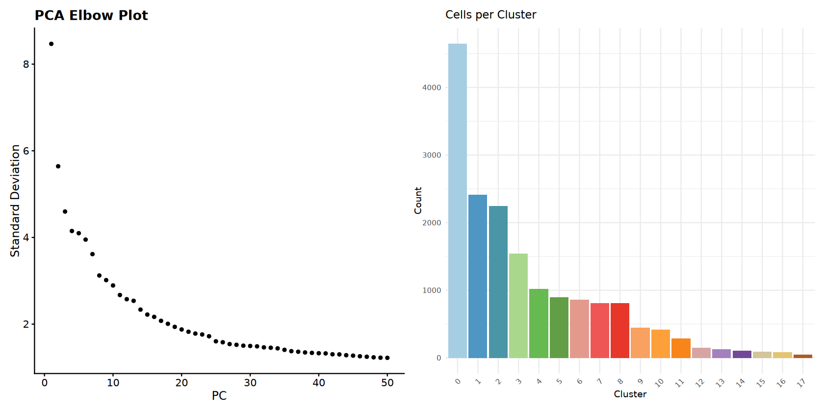
# Elbow plot
p_elbow <- ElbowPlot(combined_samples, ndims = 50) +
          ggtitle("PCA Elbow Plot")

# Cell count bar plot
cluster_data <- data.frame(
    Cluster = names(cluster_sizes),
    Count = as.numeric(cluster_sizes)
)

cluster_data <- cluster_data %>%
    arrange(desc(Count)) %>%
    mutate(Cluster = factor(Cluster, levels = Cluster))

p_barplot <- ggplot(cluster_data, aes(x = Cluster, y = Count, fill = Cluster)) +
            geom_bar(stat = "identity") +
            scale_fill_manual(values = cluster_colors) +
            ggtitle("Cells per Cluster") +
            theme_minimal() +
            theme(legend.position = "none",
                  axis.text.x = element_text(angle = 45, hjust = 1))

# Display plots
print(p_clusters + p_samples)
print(p_elbow + p_barplot)

# Save all plots
ggsave(filename = file.path(output_path, "Step6_UMAP_clusters_samples.pdf"), 
       plot = p_clusters + p_samples, width = 12, height = 6)
ggsave(filename = file.path(output_path, "Step6_Elbow_and_barplot.pdf"), 
       plot = p_elbow + p_barplot, width = 12, height = 6)

print("Clustering visualization completed!")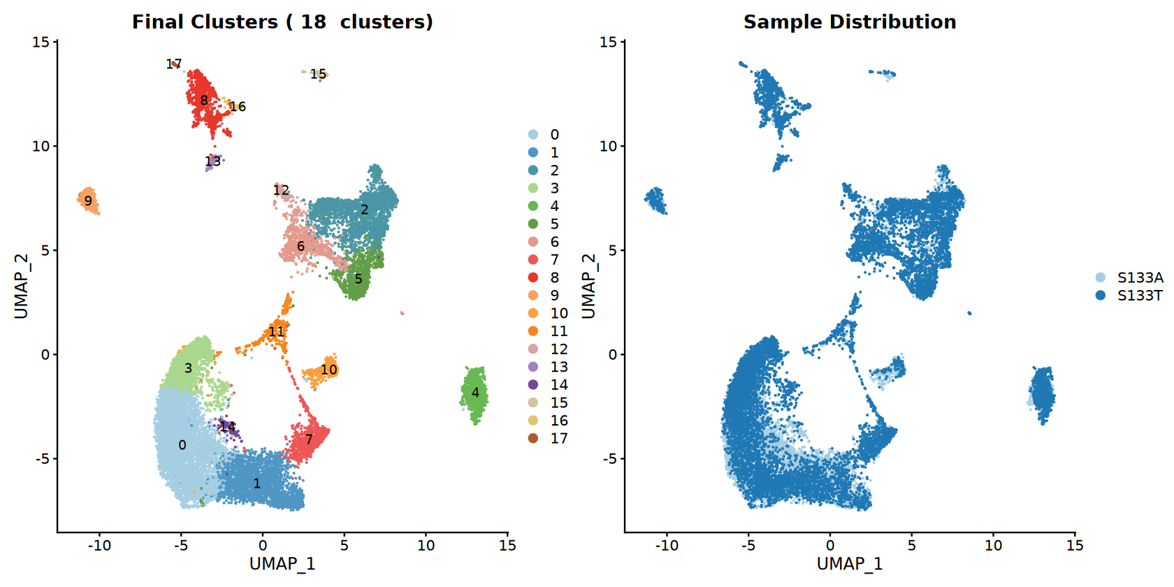

[1] "Clustering visualization completed!"

查找簇标记

识别每个簇的标记基因。

# Find markers
DefaultAssay(combined_samples) <- "RNA"
cluster_markers <- FindAllMarkers(combined_samples, only.pos = TRUE, min.pct = 0.25, logfc.threshold = 0.25)

# Top markers per cluster
top_markers <- cluster_markers %>%
    group_by(cluster) %>%
    slice_max(n = 5, order_by = avg_log2FC)

write.csv(cluster_markers, file = file.path(output_path, "Step7_cluster_markers_enhanced.csv"), row.names = FALSE)
write.csv(top_markers, file = file.path(output_path, "Step7_top_markers_enhanced.csv"), row.names = FALSE)

print("=== MARKER GENE ANALYSIS ===")
print(paste("Total markers found:", nrow(cluster_markers)))
print(paste("Clusters analyzed:", length(unique(cluster_markers$cluster))))
print("Top 5 markers per cluster:")
print(top_markers)

output

Calculating cluster 0

Calculating cluster 1

Calculating cluster 2

Calculating cluster 3

Calculating cluster 4

Calculating cluster 5

Calculating cluster 6

Calculating cluster 7

Calculating cluster 8

Calculating cluster 9

Calculating cluster 10

Calculating cluster 11

Calculating cluster 12

Calculating cluster 13

Calculating cluster 14

Calculating cluster 15

Calculating cluster 16

Calculating cluster 17

[1] "=== MARKER GENE ANALYSIS ==="
[1] "Total markers found: 8795"
[1] "Clusters analyzed: 18"
[1] "Top 5 markers per cluster:"
# A tibble: 90 × 7
# Groups: cluster [18]
p_val avg_log2FC pct.1 pct.2 p_val_adj cluster gene

1 0 1.51 0.68 0.368 0 0 IL7R
2 4.11e-264 1.13 0.73 0.59 9.91e-260 0 CXCR4
3 3.10e-176 1.11 0.404 0.224 7.48e-172 0 RORA
4 1.64e-133 1.10 0.363 0.204 3.95e-129 0 ICOS
5 1.29e- 71 1.10 0.836 0.844 3.10e- 67 0 FOS
6 0 2.92 0.801 0.149 0 1 NKG7
7 0 2.59 0.781 0.322 0 1 CCL4
8 0 2.49 0.49 0.077 0 1 IFNG
9 0 2.49 0.255 0.025 0 1 XCL2
10 0 2.44 0.608 0.068 0 1 GZMH
# ℹ 80 more rows
[1] "=== MARKER GENE ANALYSIS ==="
[1] "Total markers found: 8253"
[1] "Clusters analyzed: 15"
[1] "Top 5 markers per cluster:"
# A tibble: 75 × 7
# Groups: cluster [15]
p_val avg_log2FC pct.1 pct.2 p_val_adj cluster gene

1 0 1.27 0.686 0.391 0 0 IL7R
2 2.29e- 54 1.12 0.838 0.843 5.53e- 50 0 FOS
3 6.87e-219 1.08 0.743 0.589 1.65e-214 0 CXCR4
4 9.57e-238 1.04 0.858 0.808 2.30e-233 0 TSC22D3
5 2.08e-111 1.01 0.675 0.549 5.01e-107 0 CD69
6 0 2.55 0.682 0.146 0 1 NKG7
7 0 2.33 0.415 0.076 0 1 IFNG
8 0 2.26 0.682 0.328 0 1 CCL4
9 0 2.23 0.497 0.068 0 1 GZMH
10 0 2.21 0.867 0.245 0 1 CCL5
# ℹ 65 more rows

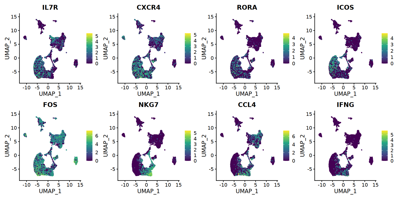
Marker Gene Visualization

Comprehensive visualization of marker genes.

# Top markers for visualization
if (nrow(top_markers) >= 8) {
    selected_genes <- top_markers$gene[1:8]  # First 8 top markers
    
    # Feature plots with continuous colors
    options(repr.plot.width = 14, repr.plot.height = 7)
    feature_plots <- FeaturePlot(combined_samples, 
                                 features = selected_genes, 
                                 ncol = 4,
                                 reduction = "umap") & 
                    scale_color_viridis_c(option = CONTINUOUS_COLOR)
    
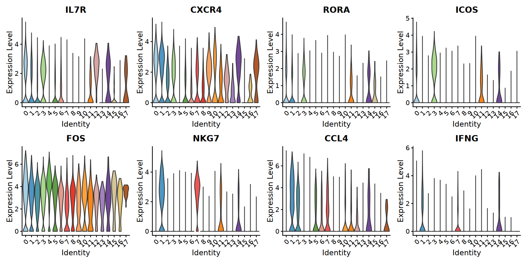
    # Violin plots with discrete colors
    violin_plots <- VlnPlot(combined_samples, 
                           features = selected_genes, 
                           ncol = 4, 
                           cols = cluster_colors,
                           pt.size = 0)
    
    print(feature_plots)
    print(violin_plots)
    
    # Save plots
    ggsave(filename = file.path(output_path, "Step7_Marker_genes_FeaturePlot.pdf"), 
           plot = feature_plots, width = 16, height = 8)
    ggsave(filename = file.path(output_path, "Step7_Marker_genes_ViolinPlot.pdf"), 
           plot = violin_plots, width = 16, height = 8)
}

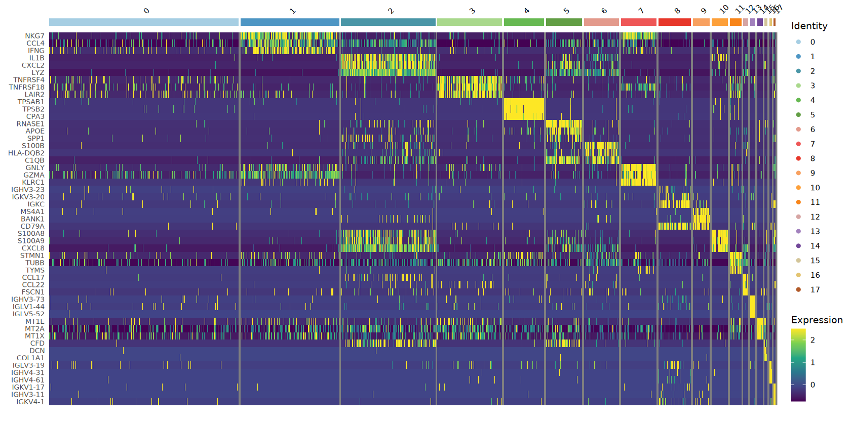
# Heatmap of top markers
top3_markers <- cluster_markers %>%
    group_by(cluster) %>%
    slice_max(n = 3, order_by = avg_log2FC)

if (nrow(top3_markers) > 0) {
    tryCatch({
        # Downsample for heatmap if too many cells
        if (ncol(combined_samples) > 5000) {
            sample_cells <- sample(colnames(combined_samples), 5000)
            heatmap_object <- subset(combined_samples, cells = sample_cells)
        } else {
            heatmap_object <- combined_samples
        }
        
        heatmap_plot <- DoHeatmap(heatmap_object, 
                                  features = top3_markers$gene, 
                                  group.colors = cluster_colors,
                                  size = 3) + 
                        scale_fill_viridis_c(option = CONTINUOUS_COLOR) +
                        theme(axis.text.y = element_text(size = 8))
        
        print(heatmap_plot)
        ggsave(filename = file.path(output_path, "Step7_Marker_genes_Heatmap.pdf"), 
               plot = heatmap_plot, width = 12, height = 10)
        
    }, error = function(e) {
        print(paste("Could not create heatmap:", e$message))
    })
}

print("Marker gene visualizations completed!")

output

Scale for colour is already present.
Adding another scale for colour, which will replace the existing scale.
Scale for colour is already present.
Adding another scale for colour, which will replace the existing scale.
Scale for colour is already present.
Adding another scale for colour, which will replace the existing scale.
Scale for colour is already present.
Adding another scale for colour, which will replace the existing scale.
Scale for colour is already present.
Adding another scale for colour, which will replace the existing scale.
Scale for colour is already present.
Adding another scale for colour, which will replace the existing scale.
Scale for colour is already present.
Adding another scale for colour, which will replace the existing scale.
Scale for colour is already present.
Adding another scale for colour, which will replace the existing scale.

Warning message in DoHeatmap(heatmap_object, features = top3_markers$gene, group.colors = cluster_colors, :
“The following features were omitted as they were not found in the scale.data slot for the RNA assay: RORA, CXCR4, IL7R”
[1m[22mScale for [32mfill[39m is already present.
Adding another scale for [32mfill[39m, which will replace the existing scale.

[1] "Marker gene visualizations completed!"

保存结果

Save all analysis results and create final summary.

# Save Seurat object
saveRDS(combined_samples, file = file.path(output_path, "Step8_Seurat.rds"))

# Create comprehensive summary
final_cells <- ncol(combined_samples)
cells_retained_percent <- round((final_cells / pre_filter_cells) * 100, 2)

summary_stats <- data.frame(
    Metric = c(
        "Species", "Samples Processed", "Sample Names", 
        "Total Cells (Final)", "Total Genes", "Cells Retained (%)", 
        "Number of Clusters", "DoubletFinder Enabled", 
        "Integration Method", "Clustering Resolution", "PCA Dimensions Used", 
        "Discrete Color Scheme", "Continuous Color Scheme"
    ),
    Value = c(
        species, length(successful_samples), paste(successful_samples, collapse = ", "),
        final_cells, nrow(combined_samples), cells_retained_percent,
        length(unique(Idents(combined_samples))), enable_doublet_detection,
        integration_method, clustering_resolution, paste(range(dims_use), collapse = "-"), 
        DISCRETE_COLOR, CONTINUOUS_COLOR
    )
)

# Save files
write.csv(summary_stats, file = file.path(output_path, "Step8_analysis_summary_enhanced.csv"), row.names = FALSE)

print("=== ANALYSIS COMPLETED SUCCESSFULLY ===")
print("")
print("Visualization files saved:")
print("- Step2 and Step3 QC plots: Before/after filtering comparison")
print("- Step4 DoubletFinder plots: UMAP visualization and score distributions")
print("- Step6 Clustering plots: UMAP and QC metric overlays")
print("- Step7 Marker gene plots: Feature plots, violin plots, and heatmaps")
print("")
print("Files saved:")
print("- Step7_cluster_markers_enhanced.csv: All marker genes")
print("- Step7_top_markers_enhanced.csv: Top 5 markers per cluster")
print("- Step8_seurat_object_enhanced.rds: Complete Seurat object")
print("- Step8_analysis_summary_enhanced.csv: Analysis parameters and statistics")
print("")
print("=== FINAL SUMMARY ===")
print(summary_stats)

output

[1] "=== ANALYSIS COMPLETED SUCCESSFULLY ==="
[1] ""
[1] "Visualization files saved:"
[1] "- Step2 and Step3 QC plots: Before/after filtering comparison"
[1] "- Step4 DoubletFinder plots: UMAP visualization and score distributions"
[1] "- Step6 Clustering plots: UMAP and QC metric overlays"
[1] "- Step7 Marker gene plots: Feature plots, violin plots, and heatmaps"
[1] ""
[1] "Files saved:"
[1] "- Step7_cluster_markers_enhanced.csv: All marker genes"
[1] "- Step7_top_markers_enhanced.csv: Top 5 markers per cluster"
[1] "- Step8_seurat_object_enhanced.rds: Complete Seurat object"
[1] "- Step8_analysis_summary_enhanced.csv: Analysis parameters and statistics"
[1] ""
[1] "=== FINAL SUMMARY ==="
Metric Value
1 Species human
2 Samples Processed 2
3 Sample Names S133A, S133T
4 Total Cells (Final) 16924
5 Total Genes 24091
6 Cells Retained (%) 91.39
7 Number of Clusters 18
8 DoubletFinder Enabled TRUE
9 Integration Method Harmony
10 Clustering Resolution 0.5
11 PCA Dimensions Used 1-30
12 Discrete Color Scheme Paired
13 Continuous Color Scheme viridis

模板信息

Template Launch Date: August 19, 2025
Last Updated: August 19, 2025

Contact: For questions, issues, or suggestions regarding this tutorial, please contact us through the "智能咨询(Intelligent Consultation)" service.

参考资料

[1] Seurat 包: https://github.com/satijalab/seurat.

[2] DoubletFinder: https://github.com/chris-mcginnis-ucsf/DoubletFinder.

[3] Harmony: https://github.com/immunogenomics/harmony. : scRNA-seq data analysis and visualization were performed by SeekSoul®Online(https://seeksoul.online/index.html#/sgvps/home).

Seurat 单细胞转录组分析全流程教程 (QC / 整合 / 聚类) ​

Seurat 简介 ​

内核配置 ​

参数配置 ​

Seurat 综合分析流程 ​

加载库和数据 ​

创建 Seurat 对象并进行质控 ​

过滤前的质控可视化 ​

细胞过滤 ​

QC Visualization After Filtering ​

DoubletFinder 分析 ​

数据整合 ​

聚类分析 ​

Clustering Visualization ​

查找簇标记 ​

Marker Gene Visualization ​

保存结果 ​

模板信息 ​

参考资料 ​

Seurat 单细胞转录组分析全流程教程 (QC / 整合 / 聚类)

Seurat 简介

内核配置

参数配置

Seurat 综合分析流程

加载库和数据

创建 Seurat 对象并进行质控

过滤前的质控可视化

细胞过滤

QC Visualization After Filtering

DoubletFinder 分析

数据整合

聚类分析

Clustering Visualization

查找簇标记

Marker Gene Visualization

保存结果

模板信息

参考资料