ATAC + RNA Multi-omics: Trios Analysis

Author: SeekGene

Time: 61 min

Words: 12.0k words

Updated: 2026-07-07

Reads: 0 times

1. Tutorial Overview

This tutorial leverages the SeekArc single-cell multi-omics dataset (scRNA-seq + scATAC-seq) to unravel the transcriptional regulatory logic underlying cell-state-specific gene expression programs. The TF–Peak–Gene trio serves as the core functional unit for dissecting this regulatory network:

TF (Regulatory Initiator): Transcription factors initiate specific regulatory events by recognizing and binding to characteristic motifs on target DNA.
Peak (Regulatory Medium): Represents an accessible chromatin region, typically enriched for cis-regulatory elements such as enhancers and promoters; its accessibility constitutes the physical prerequisite for TF function.
Gene (Functional Output): Changes in gene expression represent the ultimate transcriptional readout of upstream regulatory events.

The central goal of this tutorial is to systematically identify, within a defined cellular context, which TFs bind to which regulatory Peaks to ultimately regulate which Genes, thereby reconstructing a biologically interpretable regulatory logic chain.

suppressPackageStartupMessages(suppressWarnings({
    library(presto)
    library(ggrepel)
    library(Seurat)
    library(BiocGenerics)
    library(S4Vectors)
    library(IRanges)
    library(Signac)
    library(ComplexHeatmap)
    library(RColorBrewer)
    library(GenomicRanges)
    library(igraph)
    library(Biobase)
    library(AnnotationDbi)
    library(org.Hs.eg.db)
    #library(org.Mm.eg.db)
    library(JASPAR2020)
    library(TFBSTools)
    library(memuse)
    library(stringr)
    library(dplyr)
    library(DOSE)
    library(clusterProfiler)
    library(enrichplot)
    library(foreach)
    library(doParallel)
    library(circlize)
}))

2. Input File Preparation

First, configure the parallel computing parameters and file paths. The following result files are required:

Gene2PeakLinks.xls: Peak-to-Gene (P2G) analysis output.
output.rds: Seurat object containing single-cell RNA and ATAC multi-modal data, together with Motif annotations.

## species: Species information, "human" or "mouse" etc., used for TF name case conversion and downstream enrichment analysis
species = "human"

## links_path: Path to the Gene2PeakLinks.xls file output by the Peak2Gene module, containing Peak–Gene correlation links
links_path = "/path/to/Gene2PeakLinks.xls"

## rds_path: Path to the input Seurat object RDS file, containing pre-processed single-cell multi-omics data and Motif annotations
rds_path = "/path/to/output.rds"

## pseudobulk_size: Pseudobulk size, indicating how many cells are aggregated per group for correlation computation (recommended: 10; set to 1 to disable)
pseudobulk_size = 10

## min_motif_score: Minimum Motif Score threshold, used to filter low-affinity TF–Peak bindings (recommended: 10.0; set to 0 to disable filtering)
min_motif_score = 10.0

## min_tf_gene_cor: Minimum absolute threshold for TF–Gene expression correlation, used to filter TF–target gene pairs with co-variation at the expression level (recommended: 0.2)
min_tf_gene_cor = 0.2

## min_tf_activity_cor: Minimum absolute threshold for TF activity–expression consistency correlation (recommended: 0.2)
min_tf_activity_cor = 0.2

## min_tf_activity_target_cor: Minimum absolute threshold for TF activity–target gene expression correlation (recommended: 0.2)
min_tf_activity_target_cor = 0.2

## max_tf_gene_pvalue: Maximum P-value threshold for TF–Gene expression correlation (recommended: 0.05)
max_tf_gene_pvalue = 0.05

## max_tf_activity_pvalue: Maximum P-value threshold for TF activity–expression consistency (recommended: 0.05)
max_tf_activity_pvalue = 0.05

## max_tf_activity_target_pvalue: Maximum P-value threshold for TF activity–target gene expression correlation (recommended: 0.05)
max_tf_activity_target_pvalue = 0.05

## heatmap_group_by: Column name used to group the heatmap by cell population; must exist in the Seurat object's meta.data
heatmap_group_by = "Celltype"

## celltype_col: Cell-type column name, typically consistent with heatmap_group_by
celltype_col = "Celltype"

💡 Note Fill in the parameters here according to your own needs.


set.seed(1234)

cores <- 8                    
gene_block <- 2000      


heatmap_pseudobulk_size <- 10      
output_path <- "./result/"
heatmap_out_dir <- file.path(output_path, "TF_Targetcds_Heatmaps")
scatter_out_dir <- file.path(output_path, "TF_Targets_Scatters")
network_out_dir <- file.path(output_path, "TF_Targets_Networks")
top_tf_detail_n <- 25
network_max_nodes <- 50
top_n_trios <- 100                 
top_n_genes_per_tf_heatmap <- 500
global_network_max_tfs <- 25
global_network_max_targets_per_tf <- 15

💡 Note Modifying these parameters is not recommended.

3. Initial Trio Assembly

Building on the prior Peak-to-Gene (P2G) analysis results, we first extract putative regulatory links that exhibit both spatial proximity and accessibility–expression correlation. We then identify motifs that fall within Peak regions through spatial overlap, generating the initial TF–Peak–Gene trios.

3.1 Loading the Peak2Gene Result File (Gene2PeakLinks.xls)

This file contains co-variation links between Peaks and Genes, where the score column represents the correlation between the two. Unnecessary columns are removed and the essential ones are retained.

options(warn = -1) 
links_df <- read.delim(links_path,stringsAsFactors = FALSE)
colnames(links_df)[which(colnames(links_df) == "score")]="peak_gene_cor"
head(links_df)

A data.frame: 6 × 10
	seqnames	start	end	width	strand	peak_gene_cor	gene	peak	zscore	pvalue
	<chr>	<int>	<int>	<int>	<chr>	<dbl>	<chr>	<chr>	<dbl>	<dbl>
1	chr1	630741	778747	148007	*	0.05754247	LINC01409	chr1-630357-631124	3.234682	0.000608892
2	chr1	630741	825138	194398	*	0.07142624	LINC01128	chr1-630357-631124	2.048501	0.020255460
3	chr1	634028	911435	277408	*	0.05839843	AL645608.2	chr1-633645-634410	2.261820	0.011854276
4	chr1	778747	923875	145129	*	0.05357620	LINC01409	chr1-923441-924308	1.888788	0.029460142
5	chr1	778747	1019770	241024	*	0.05575774	LINC01409	chr1-1019073-1020467	1.712726	0.043381452
6	chr1	778747	1144376	365630	*	0.06227576	LINC01409	chr1-1143762-1144990	2.131101	0.016540407

links_df <- links_df[,c("peak_gene_cor","gene","peak","zscore","pvalue")]

3.2 Loading Multi-Omics Data and Motif–Peak Spatial Mapping

Read the pre-processed single-cell multi-omics data (Seurat object), extract transcription factor (TF) binding motif information, and perform a genomic spatial overlap alignment between these motifs and the candidate regulatory Peaks.

Core Steps Breakdown:

Loading the Seurat Object: Read the .rds file and switch the default analysis assay to ATAC.
💡 Note: The input Seurat object must have undergone AddMotifs in the upstream analysis to ensure it contains complete motif sequence annotations and genome-wide position information.
Extracting Motif Coordinates and Binding Scores: Use Motifs() to extract the motif list stored in the object, obtain the precise genomic coordinates of all TF binding sites, and flatten them into a GRanges (Genomic Ranges) object. At the same time, retrieve the mapping dictionary from motif IDs to true TF names, as well as the sequence affinity score (motif_score) for each binding site.
Constructing Peak Genomic Intervals: Extract all de-duplicated Peak names from the Peak-to-Gene (P2G) table of the previous step. Since the original Peak names are plain strings, convert them into standard GRanges genomic interval objects via string splitting so that interval arithmetic can be performed downstream.
💡 Format Tip: In this tutorial, Peak names follow the hyphen-separated format (e.g., chr1-1000-2000). If your upstream data use the standard colon–hyphen format (e.g., chr1:1000-2000), please modify the regular expression in the strsplit function below, or replace the : in the names with - before passing them in.
Physical Spatial Overlap Alignment (findOverlaps): This is the key step for establishing the physical regulatory evidence of trios! Using the findOverlaps function, compute the intersection between the genome-wide motif intervals and the Peak intervals of interest. This allows us to pinpoint precisely: which TF binding sites fall exactly within our target regulatory Peaks, thereby successfully establishing the "TF → Peak" physical binding relationship.

data <- readRDS(rds_path)
DefaultAssay(data) <- "ATAC"

motif_info <- Motifs(data)
motif_positions <- motif_info@positions

motif_tf_map <- vapply(motif_info@motif.names, function(x) x[[1]], character(1))

motif_pos_gr <- unlist(motif_positions)

motif_gr <- motif_pos_gr
motif_gr$motif_id <- names(motif_pos_gr)
motif_gr$TF_raw <- motif_tf_map[motif_gr$motif_id]
motif_gr$motif_score <- motif_gr$score

unique_peaks_links <- unique(links_df$peak)
peak_coords <- strsplit(unique_peaks_links, "-")
links_peaks_gr <- GRanges(
  seqnames = sapply(peak_coords, `[`, 1),
  ranges = IRanges(start = as.integer(sapply(peak_coords, `[`, 2)), 
                   end = as.integer(sapply(peak_coords, `[`, 3))),
  peak = unique_peaks_links
)

olap <- findOverlaps(motif_gr, links_peaks_gr)
                       
tf_peak_df <- data.frame(
  peak = links_peaks_gr$peak[subjectHits(olap)],
  motif_id = motif_gr$motif_id[queryHits(olap)],
  TF_raw = motif_gr$TF_raw[queryHits(olap)],
  motif_score = motif_gr$motif_score[queryHits(olap)],
  stringsAsFactors = FALSE
)

3.3 Completing Initial Trio Assembly and Background Noise Filtering

With the spatial mapping between motifs and Peaks established, we now know "which TFs bind to which Peaks." Next, we need to standardize TF nomenclature, bridge the TF–Peak relationship with the earlier Peak–Gene relationship, and use the actual single-cell transcriptomic data to eliminate "false-positive" regulatory noise.

Core Steps Breakdown:

TF Name Cleaning and Standardization:
- Removing Non-Standard Characters: TF names from public databases (e.g., JASPAR/CIS-BP) often carry family suffixes (e.g., :: symbols) or parenthetical notes. The code strips these via regular expressions to extract the clean TF short name.
- Cross-Species Homolog Alignment: To ensure accuracy in downstream RNA expression extraction and functional enrichment analysis, TF names must have their letter casing aligned with the gene nomenclature conventions of the target species (e.g., first-letter capitalization for mouse/rat, all-lowercase for zebrafish, all-uppercase for human).
- Removing Redundant Binding Sites: If multiple similar motif sequence matches exist for the same TF within the same Peak, we conservatively retain only the one with the highest score (max(motif_score)) as the representative.
Assembling the Initial TF–Peak–Gene Trios: Using the shared regulatory element peak as the bridge, merge the TF–Peak mapping table with the Peak–Gene link table via an inner join (inner_join). At this point, the complete TF -> Peak -> Gene logic chain is tentatively assembled.
Expression Noise Filtering Based on scRNA-seq:
- Biological Rationale: Even if a TF has a strong motif binding site in the genome, if that TF is not transcribed at all in the cell sample under study, such "physical binding potential" constitutes biologically meaningless background noise (false positive).
- Operational Logic: The code extracts the measured single-cell RNA expression matrix from the Seurat object and performs a strict intersection filter (intersect) on the initially assembled trios. Only TFs and target genes that are actually detected as expressed in the current cellular system are retained, substantially improving the authenticity of the candidate regulatory network.

tf_peak_df <- tf_peak_df %>% 
  mutate(TF = sapply(strsplit(TF_raw, "::"), `[`, 1)) %>% 
  mutate(TF = trimws(gsub("\\s*\\(.*\\)", "", TF))) %>%
  mutate(TF = if (tolower(species) %in% c("mouse", "rat")) { 
    paste0( 
      toupper(substr(tolower(TF), 1, 1)), 
      substr(tolower(TF), 2, nchar(tolower(TF))) 
    ) 
  } else if (tolower(species) == "zebrafish") { 
    tolower(TF) 
  } else { 
    toupper(TF) 
  }) %>% 
  group_by(peak, TF, motif_id) %>% 
  summarize(motif_score = max(motif_score), .groups = "drop")

trios_df <- links_df %>%
  inner_join(tf_peak_df, by = "peak", relationship = "many-to-many") %>%
  filter(motif_score >= min_motif_score)

rna_data <- tryCatch({
    GetAssayData(data, assay = "RNA", layer = "data")
}, error = function(e) {
GetAssayData(data, assay = "RNA", slot = "data")
})

unique_tfs <- intersect(unique(trios_df$TF), rownames(rna_data))
unique_genes <- intersect(unique(trios_df$gene), rownames(rna_data))
trios_df <- trios_df %>%
    filter(TF %in% unique_tfs & gene %in% unique_genes)

expr_tfs <- as.matrix(rna_data[unique_tfs, , drop = FALSE])
expr_genes <- as.matrix(rna_data[unique_genes, , drop = FALSE])
if (pseudobulk_size > 1) {
    meta <- data@meta.data
    group_col <- if (exists("celltype_col") && celltype_col %in% colnames(meta)) celltype_col else {
        found <- intersect(c("seurat_clusters", "Cluster", "CellType", "celltype", "Annotation", "Celltype"), colnames(meta))
        if (length(found) > 0) found[1] else NA
    }
    
    if (!is.na(group_col) && !is.null(group_col)) {
        cell_groups <- split(colnames(expr_tfs), meta[colnames(expr_tfs), group_col])
        groups <- list()
        for (ct in names(cell_groups)) {
            cells <- cell_groups[[ct]]
            n_cells <- length(cells)
            if (n_cells > 0) {
                if (n_cells < pseudobulk_size) {
                    groups[[paste0(ct, "_1")]] <- cells
                } else {
                    n_pbs <- ceiling(n_cells / pseudobulk_size)
                    split_idx <- as.numeric(cut(seq_along(cells), breaks = n_pbs))
                    chunked_cells <- split(cells, split_idx)
                    for (i in names(chunked_cells)) {
                        groups[[paste0(ct, "_", i)]] <- chunked_cells[[i]]
                    }
                }
            }
        }
    } else {
        ncol_all <- ncol(expr_tfs)
        groups <- split(seq_len(ncol_all), ceiling(seq_len(ncol_all) / pseudobulk_size))
        groups <- lapply(groups, function(idx) colnames(expr_tfs)[idx])
    }
    
    expr_tfs_list <- lapply(groups, function(g) {
        valid_g <- intersect(g, colnames(expr_tfs))
        if (length(valid_g) > 1) rowMeans(expr_tfs[, valid_g, drop = FALSE]) else if (length(valid_g) == 1) expr_tfs[, valid_g] else rep(0, nrow(expr_tfs))
    })
    expr_genes_list <- lapply(groups, function(g) {
        valid_g <- intersect(g, colnames(expr_genes))
        if (length(valid_g) > 1) rowMeans(expr_genes[, valid_g, drop = FALSE]) else if (length(valid_g) == 1) expr_genes[, valid_g] else rep(0, nrow(expr_genes))
    })
    
    expr_tfs <- do.call(cbind, expr_tfs_list)
    expr_genes <- do.call(cbind, expr_genes_list)
    colnames(expr_tfs) <- paste0("bulk", seq_len(ncol(expr_tfs)))
    colnames(expr_genes) <- paste0("bulk", seq_len(ncol(expr_genes)))
} else {
    zhanwei="zhanwei"
}
tf_gene_pairs <- trios_df %>% 
    dplyr::select(TF, gene) %>% 
    distinct()
options(warn = 0)

4. Active Regulatory Filtering and Statistical Testing

Possessing only a "physical spatial mapping (motif within a peak)" is insufficient. In single-cell multi-omics data, genuine cis-regulatory networks are typically accompanied by co-variation. Therefore, we need to compute the expression correlation and its statistical significance for every candidate TF–Gene pair, providing a numerical basis for the subsequent high-confidence filtering.

4.1 Computing TF–Target Gene Expression Correlation (TF–Gene Correlation)

This section computes the Pearson correlation between the mRNA expression of a transcription factor (TF) and that of its target gene across cells (or pseudobulk groups).

Core Computational Logic:

Matrix Chunking and Parallel Acceleration: Given the large number of genes, full-matrix computation is highly prone to memory overflow. The code splits genes into multiple chunks (gene_block), computes the correlation matrices in parallel via multi-threading (mclapply), and includes a built-in automatic fallback to single-core execution.
P-value Significance Testing: Using the t-distribution formula, compute the corresponding p-value from the Pearson correlation coefficient ( $r$ ) and the degrees of freedom (number of cells/groups − 2), to evaluate the statistical significance of the correlation.
Data Merging and Activity Matrix Preparation: The computed correlation coefficients (tf_gene_cor) and p-values are pasted back into the main data frame trios_df.

n_obs <- ncol(expr_tfs)
tf_index <- setNames(seq_along(unique_tfs), unique_tfs)
gene_index <- setNames(seq_along(unique_genes), unique_genes)
tf_ids <- as.integer(tf_index[tf_gene_pairs$TF])
gene_ids <- as.integer(gene_index[tf_gene_pairs$gene])

if (gene_block <= 0) {
    rmat <- cor(t(expr_tfs), t(expr_genes))
    r_out <- rmat[cbind(tf_ids, gene_ids)]
    rm(rmat)
} else {
    n_genes <- length(unique_genes)
    blocks <- split(seq_len(n_genes), ceiling(seq_len(n_genes) / gene_block))
    
    calc_block_cor <- function(idx) {
      genes <- unique_genes[idx]
      cm <- suppressWarnings(cor(t(expr_tfs), t(expr_genes[genes, , drop = FALSE])))
      pos <- which(gene_ids %in% idx)
      if (length(pos) == 0) {
        list(pos = integer(0), r = numeric(0))
      } else {
        gi <- match(gene_ids[pos], idx)
        ri <- cm[cbind(tf_ids[pos], gi)]
        list(pos = pos, r = ri)
      }
    }
    if (cores > 1) {
       res_list <- tryCatch({
         parallel::mclapply(blocks, calc_block_cor, mc.cores = cores, mc.preschedule = TRUE)
       }, warning = function(w) {
         return(NULL)
       }, error = function(e) {
         return(NULL)
       })
       
       if (is.null(res_list) || any(sapply(res_list, function(x) inherits(x, "try-error")))) {
         res_list <- lapply(blocks, calc_block_cor)
       }
    } else {
       res_list <- lapply(blocks, calc_block_cor)
    }

    r_out <- numeric(length(tf_ids))
    for (el in res_list) {
      if (!is.null(el) && length(el$pos) > 0) r_out[el$pos] <- el$r
    }
}

df <- n_obs - 2
if (df > 0) {
    r_clip <- pmin(pmax(r_out, -0.999999), 0.999999)
    tstat <- r_clip * sqrt(df / (1 - r_clip^2))
    p_out <- 2 * pt(-abs(tstat), df)
} else {
    p_out <- rep(NA_real_, length(r_out))
}
tf_gene_pairs$tf_gene_cor <- r_out
tf_gene_pairs$tf_gene_pvalue <- p_out
trios_df <- trios_df %>% 
left_join(tf_gene_pairs, by = c("TF", "gene"))

head(trios_df)

A data.frame: 6 × 10
	peak_gene_cor	gene	peak	zscore	pvalue	TF	motif_id	motif_score	tf_gene_cor	tf_gene_pvalue
	<dbl>	<chr>	<chr>	<dbl>	<dbl>	<chr>	<chr>	<dbl>	<dbl>	<dbl>
1	0.05754247	LINC01409	chr1-630357-631124	3.234682	0.000608892	ALX3	MA0634.1	11.53991	-0.001394294	0.964857861
2	0.05754247	LINC01409	chr1-630357-631124	3.234682	0.000608892	E2F4	MA0470.1	13.64899	0.096255918	0.002298513
3	0.05754247	LINC01409	chr1-630357-631124	3.234682	0.000608892	E2F6	MA0471.1	14.39160	0.051465457	0.103665294
4	0.05754247	LINC01409	chr1-630357-631124	3.234682	0.000608892	GATA1	MA0035.4	12.35489	0.088867335	0.004897611
5	0.05754247	LINC01409	chr1-630357-631124	3.234682	0.000608892	GSX1	MA0892.1	10.50603	0.057667498	0.068188944
6	0.05754247	LINC01409	chr1-630357-631124	3.234682	0.000608892	GSX2	MA0893.1	10.66570	-0.014060515	0.656810574

4.2 Computing Consistency Correlation between TF Activity and Its Own Expression

Correlation of target gene expression alone is not enough. When an active transcription factor (TF) exerts its regulatory function, its own mRNA expression level is typically highly consistent with its genome-wide chromatin binding activity (ChromVAR motif activity).

The code in this section extracts the ChromVAR activity matrix inferred from scATAC-seq and performs the following operations:

Dimension Alignment and Denoising: The ChromVAR activity matrix is aggregated by mean using exactly the same pseudobulk grouping strategy as the RNA matrix, to eliminate the extreme sparsity of single-cell data.
Consistency Evaluation: For each TF–Motif pair, compute the Pearson correlation (tf_activity_cor) and significance (tf_activity_pvalue) between its RNA expression level and its motif accessibility activity.

💡 Biological Significance: If the correlation is significantly positive, it indicates that the higher the TF's expression, the more accessible its genome-wide binding sites — providing strong epigenetic evidence that the TF is a "genuinely active regulatory factor."

chromvar_data <- GetAssayData(data, assay = "chromvar", layer = "data")

valid_motifs <- intersect(unique(trios_df$motif_id), rownames(chromvar_data))
if (length(valid_motifs) > 0) {
    expr_motifs <- as.matrix(chromvar_data[valid_motifs, , drop = FALSE])

    if (pseudobulk_size > 1 && exists("groups")) {
       expr_motifs_list <- lapply(groups, function(g) rowMeans(expr_motifs[, g, drop = FALSE]))
       expr_motifs <- do.call(cbind, expr_motifs_list)
       mode(expr_motifs) <- "numeric"
       colnames(expr_motifs) <- paste0("bulk", seq_len(ncol(expr_motifs)))
    }

    common_cols <- intersect(colnames(expr_tfs), colnames(expr_motifs))
    expr_tfs_align <- expr_tfs[, common_cols, drop = FALSE]
    expr_motifs_align <- expr_motifs[, common_cols, drop = FALSE]

    tf_motif_pairs <- trios_df %>% 
      filter(motif_id %in% valid_motifs & TF %in% rownames(expr_tfs_align)) %>%
      dplyr::select(TF, motif_id) %>% 
      distinct()    
    if (length(common_cols) >= 3) {
        tf_act_cor <- numeric(nrow(tf_motif_pairs))
        tf_act_pval <- numeric(nrow(tf_motif_pairs))
        
        for (i in seq_len(nrow(tf_motif_pairs))) {
          tf <- tf_motif_pairs$TF[i]
          motif <- tf_motif_pairs$motif_id[i]
          
          #res <- cor.test(expr_tfs_align[tf, ], expr_motifs_align[motif, ], method = "pearson")
          res <- suppressWarnings(
              cor.test(expr_tfs_align[tf, ], expr_motifs_align[motif, ], method = "pearson")
          )
          if (is.na(res$estimate)) {
             tf_act_cor[i] <- 0
             tf_act_pval[i] <- 1
          } else {
             tf_act_cor[i] <- res$estimate
             tf_act_pval[i] <- res$p.value
          }
        }
        
        tf_motif_pairs$tf_activity_cor <- tf_act_cor
        tf_motif_pairs$tf_activity_pvalue <- tf_act_pval

        trios_df <- trios_df %>%
          left_join(tf_motif_pairs, by = c("TF", "motif_id"))
    } else {
        trios_df$tf_activity_cor <- NA
        trios_df$tf_activity_pvalue <- NA
    }
  } else {
    trios_df$tf_activity_cor <- NA
    trios_df$tf_activity_pvalue <- NA
  }

4.3 Computing Correlation between TF Activity and Target Gene Expression (Distinguishing Activation from Repression)

Beyond examining the TF's own expression, we are even more interested in whether the TF's chromatin-level binding activity directly drives transcription of downstream target genes. This constitutes the most direct evidence characterizing a genuine physical regulatory network.

The code in this section performs the following computations:

Data Alignment: Align the ChromVAR activity matrix with the RNA expression matrix of target genes.
Correlation Testing: For each TF–Target pair, compute the Pearson correlation and p-value between its motif activity score and the target gene's mRNA expression level.

  if (exists("expr_motifs_align") && exists("expr_genes")) {
      common_cols_target <- intersect(colnames(expr_genes), colnames(expr_motifs_align))
      
      if (length(common_cols_target) >= 3) {
          expr_genes_align <- expr_genes[, common_cols_target, drop = FALSE]
          expr_motifs_align_target <- expr_motifs_align[, common_cols_target, drop = FALSE]
          
          target_pairs <- trios_df %>%
              filter(motif_id %in% rownames(expr_motifs_align_target) & gene %in% rownames(expr_genes_align)) %>%
              dplyr::select(motif_id, gene) %>%
              distinct()
          
          
          target_cor <- numeric(nrow(target_pairs))
          target_pval <- numeric(nrow(target_pairs))

          for (i in seq_len(nrow(target_pairs))) {
              m_id <- target_pairs$motif_id[i]
              g_id <- target_pairs$gene[i]
              
              res <- suppressWarnings(cor.test(expr_motifs_align_target[m_id, ], expr_genes_align[g_id, ], method = "pearson"))
              
              if (is.na(res$estimate)) {
                 target_cor[i] <- 0
                 target_pval[i] <- 1
              } else {
                 target_cor[i] <- res$estimate
                 target_pval[i] <- res$p.value
              }
          }
          target_pairs$tf_activity_target_cor <- target_cor
          target_pairs$tf_activity_target_pvalue <- target_pval
          
          trios_df <- trios_df %>%
              left_join(target_pairs, by = c("motif_id", "gene"))
              
      } else {
          trios_df$tf_activity_target_cor <- NA
          trios_df$tf_activity_target_pvalue <- NA
      }
  } else {
      trios_df$tf_activity_target_cor <- NA
      trios_df$tf_activity_target_pvalue <- NA
  }

💡 Note:
The correlation coefficient here (tf_activity_target_cor) is critical. In downstream visualization and enrichment analysis, we will use its sign to tentatively classify target genes into putative activation mode (Activate, Cor > 0) or putative repression mode (Repress, Cor < 0).
In single-cell data analysis, a statistical "negative correlation" cannot be directly equated with a biological "direct physical repression." It may also be an artifact caused by temporal offset along a developmental trajectory, or by the TF activating an intermediate repressor (an indirect effect). Therefore, this co-variation-based mode classification is "inferred"; definitive regulatory directionality still requires wet-lab validation.

4.4 Composite Regulatory Strength Score (Linkage Score Computation)

In complex gene regulatory networks, a target gene is typically under the cooperative control of multiple cis-regulatory elements (e.g., multiple enhancers). This means the same TF may bind to multiple Peaks around a target gene to exert its function jointly.

The code in this section quantifies the total strength of such multi-point cooperative regulation by computing the Linkage Score.

Formula:

L i n k a g e S c o r e = \sum (P e a k 2 G e n e C o r^{2} \times M o t i f S c o r e)

Code Logic Breakdown:

Per-Site Contribution Calculation: First compute the independent contribution of each Peak. Multiply the square of the correlation between Peak accessibility and gene expression ( $R^{2}$ ) by the TF's binding affinity (motif_score) at that Peak.

💡 Statistical Rationale: Why is Peak2Gene Cor squared here rather than taking its absolute value? Because in statistics, the square of the correlation coefficient $R$ (i.e., $R^{2}$ , the coefficient of determination) represents the proportion of variance in the dependent variable (target gene expression) that can be explained by the independent variable (Peak accessibility). By computing $R^{2}$ , we convert the correlation into a more rigorous "variance-explained weight."

Multi-Point Aggregation: Group and aggregate by TF–Gene pair (group_by), summing the independent contributions of all Peaks through which the same TF acts on that target gene to obtain a composite linkage_score.

💡 Note: The higher the linkage_score, the more conclusive the composite physical evidence that the TF regulates the target gene — this is the single most important basis for subsequently filtering the core regulatory backbone.

  if ("peak_gene_cor" %in% colnames(trios_df)) {
      trios_df <- trios_df %>%
          mutate(linkage_contribution = (peak_gene_cor^2) * motif_score) %>%
          group_by(gene, TF) %>%
          mutate(linkage_score = sum(linkage_contribution, na.rm = TRUE)) %>%
          ungroup() %>%
          dplyr::select(-linkage_contribution)
  } else {
      trios_df$linkage_score <- 0
  }

5. Trios Filtering and High-Confidence Network Output

After completing all statistical tests and composite scoring, we obtain a massive table containing a huge number of candidate TF–Peak–Gene combinations. However, this table also contains a large amount of weak regulation and background noise.

To build a reliable transcriptional regulatory network, we must perform stringent multi-dimensional threshold filtering. A TF–Gene pair is retained as a high-confidence trio only when it passes the triple test of physical binding, expression co-variation, and activity-driven regulation.

Core Filtering Conditions Explained:

Physical Binding Strength (motif_score): Removes false-positive binding sites where the affinity between the TF and its target sequence is extremely weak.
Triple Correlation and Significance Dual Check (removes noise with $P > 0.05$ or absolute correlation below threshold):
- tf_gene_cor: Ensures the TF and target gene exhibit significant co-expression at the mRNA level.
- tf_activity_cor: Ensures the TF's expression matches its chromatin-level activity (ChromVAR).
- tf_activity_target_cor: Ensures the TF's chromatin binding activity genuinely drives transcription of the downstream target gene.
Composite Regulatory Strength (linkage_score):
- The code automatically computes the Linkage Score distribution across all TF–Gene pairs.
- An adaptive dynamic threshold is adopted (e.g., selecting the top 10% of all scores, i.e., the 90th percentile quantile(..., 0.9) as linkage_cutoff), forcibly retaining the head of the network with the most significant regulatory effects — the core network.

Through these cascaded filters, we strip away the majority of redundant data and output the most core, highest-confidence Trios results to a local file (TF_Peak_Gene_Trios_all.txt), providing a clean data foundation for subsequent network visualization and enrichment analysis.

linkage_cutoff <- -Inf
  if ("linkage_score" %in% colnames(trios_df)) { 
      unique_scores <- trios_df %>% dplyr::select(gene, TF, linkage_score) %>% distinct()
      linkage_cutoff <- quantile(unique_scores$linkage_score, 0.9, na.rm = TRUE)

  } else {
      cat("warning: no linkage_score colcum\n")
  }
  
  before_filter <- nrow(trios_df)
  trios_df_filter <- trios_df %>%
    filter(
      motif_score >= min_motif_score,
      !is.na(tf_gene_cor) & abs(tf_gene_cor) >= min_tf_gene_cor,
      !is.na(tf_gene_pvalue) & tf_gene_pvalue <= max_tf_gene_pvalue,
      !is.na(tf_activity_cor) & abs(tf_activity_cor) >= min_tf_activity_cor,
      !is.na(tf_activity_pvalue) & tf_activity_pvalue <= max_tf_activity_pvalue,
      !is.na(tf_activity_target_cor) & abs(tf_activity_target_cor) >= min_tf_activity_target_cor,
      !is.na(tf_activity_target_pvalue) & tf_activity_target_pvalue <= max_tf_activity_target_pvalue,
      linkage_score > linkage_cutoff
    )
dir.create(output_path, recursive = TRUE, showWarnings = FALSE)
write.table(trios_df, file = paste0(output_path,"/TF_Peak_Gene_Trios_all.txt"), sep = "\t", quote = FALSE, row.names = FALSE, col.names = TRUE)
write.table(trios_df_filter, file = paste0(output_path,"/TF_Peak_Gene_Trios_all_filter.txt"), sep = "\t", quote = FALSE, row.names = FALSE, col.names = TRUE)

6. Trios Visualization

After extracting the high-confidence Trios, this section uses multi-dimensional plots to intuitively reveal the regulatory patterns of transcription factors and the core target gene network.

6.1 Core TF Selection and Target Gene Regulatory Scatter Plot

In a complex network, not all transcription factors play equally important roles. To focus on the core regulatory hubs (Hub TFs), we first compute the Total Linkage Score for each TF and select the top-ranking TFs for in-depth analysis.

For these core TFs, we plot TF–target regulatory scatter plots, each vividly displaying the regulatory distribution of the TF over its putative target genes:

X-axis: Correlation between TF activity (inferred by ChromVAR) and target gene expression. Reflects the direction and magnitude of regulation.
Y-axis: Physical regulatory strength (Linkage Score). Reflects the reliability of the regulatory evidence.

options(warn = -1)
tmp <- trios_df %>%
  dplyr::group_by(TF, gene) %>%
  dplyr::summarise(
    tf_activity_target_cor = if (all(is.na(tf_activity_target_cor))) {
      NA_real_
    } else {
      tf_activity_target_cor[which.max(abs(tf_activity_target_cor))][1]
    },
    linkage_score = if (all(is.na(linkage_score))) {
      NA_real_
    } else {
      max(linkage_score, na.rm = TRUE)
    },
    .groups = "drop"
  )
plot_tf_target_scatter <- function(tf_name, tmp, output_dir = NULL) {
  plot_data <- tmp %>% 
    filter(TF == tf_name) %>% 
    dplyr::select(gene, tf_activity_target_cor, linkage_score) %>% 
    distinct() 
  
  if (nrow(plot_data) == 0) return(NULL)
  
  x_cutoff <- min_tf_activity_target_cor 
  y_cutoff <- quantile(plot_data$linkage_score, 0.9, na.rm = TRUE) 

  plot_data <- plot_data %>% 
    mutate(
      is_top = abs(tf_activity_target_cor) > x_cutoff & linkage_score > y_cutoff,
      point_group = case_when(
        tf_activity_target_cor < -x_cutoff & linkage_score > y_cutoff ~ "left_sig",
        tf_activity_target_cor > x_cutoff & linkage_score > y_cutoff ~ "right_sig",
        TRUE ~ "other"
      )
    ) 
  
  top_genes <- plot_data %>% filter(is_top) 

  p <- ggplot(plot_data, aes(x = tf_activity_target_cor, y = linkage_score)) + 
    geom_point(aes(color = point_group), alpha = 0.8, size = 2) + 
    scale_color_manual(
      values = c(left_sig = "#2166ac", right_sig = "#b2182b", other = "grey70"),
      breaks = c("left_sig", "right_sig", "other"),
      labels = c("Repress","Activate","Others"),
      name = "Point Type"
    ) + 
    geom_vline(xintercept = x_cutoff, linetype = "dashed", color = "red") + 
    geom_vline(xintercept = -x_cutoff, linetype = "dashed", color = "red") + 
    geom_hline(yintercept = y_cutoff, linetype = "dashed", color = "red") + 
    geom_text_repel(data = top_genes %>% arrange(desc(linkage_score)) %>% head(20), 
                    aes(label = gene), size = 3, box.padding = 0.5, max.overlaps = 20) + 
    labs(title = paste0(tf_name, " putative targets (", nrow(top_genes), " genes)"), 
         x = paste0(tf_name, " motif correlation to gene"), y = "Linkage score") + 
    theme_classic() + 
    theme(plot.title = element_text(hjust = 0.5, face = "bold"), legend.position = "right")
  if (!is.null(output_dir)) {
    dir.create(output_dir, recursive = TRUE, showWarnings = FALSE)
    ggsave(file.path(output_dir, paste0(tf_name, "_target_scatter.pdf")), p, width = 8, height = 5)
  }
  
  return(p)
}


top_tfs <- tmp %>% 
  group_by(TF) %>% 
  summarize(total_linkage = sum(linkage_score, na.rm = TRUE), .groups = "drop") %>% 
  arrange(desc(total_linkage)) %>% 
  head(top_tf_detail_n) %>% 
  pull(TF) 


plot_output_dir <- scatter_out_dir
dir.create(plot_output_dir, recursive = TRUE, showWarnings = FALSE)

save_and_encode_plot <- function(plot, filename_base, width = 8, height = 5) {
  full_path_pdf <- paste0(filename_base, ".pdf")
  temp_png <- tempfile(fileext = ".png")
  
  ggsave(full_path_pdf, plot, width = width, height = height)
  
  ggsave(temp_png, plot, width = width, height = height, dpi = 100) 
  return(NULL)
}


plot_list <- list()

for (tf in top_tfs) {
  p <- tryCatch({
    plot_tf_target_scatter(tf, tmp, output_dir = NULL)
  }, error = function(e) return(NULL))
  
  if (!is.null(p)) {
    file_base <- file.path(plot_output_dir, paste0(tf, "_scatter"))
    res <- save_and_encode_plot(p, file_base)
  }
}
options(warn = 0)

options(repr.plot.width = 15, repr.plot.height = 8)
p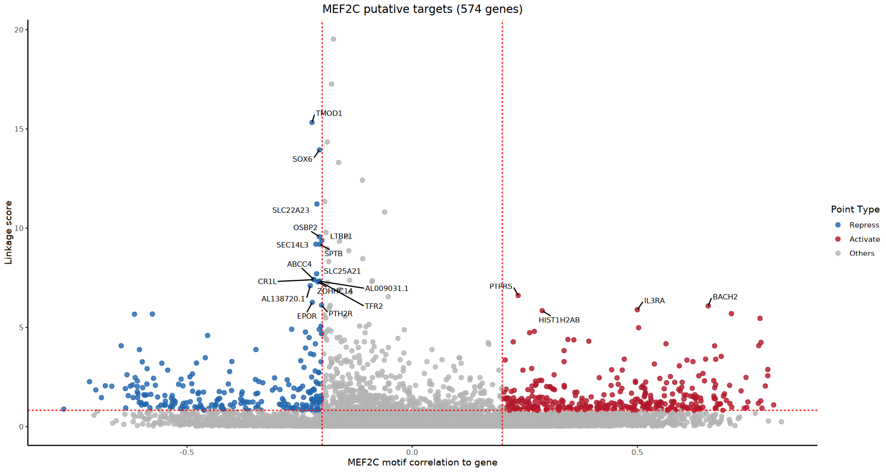

💡 Note: The example here shows the target genes regulated by one of the TFs; please refer to the ./result directory for the complete set of plots.
Activate (activation targets, red): Located in the upper-right corner (strong positive correlation + high Linkage), indicating that the TF most likely directly binds and promotes the expression of this gene.
Repress (repression targets, blue): Located in the upper-left corner (strong negative correlation + high Linkage), indicating that the TF most likely directly binds and represses the expression of this gene.
We use ggrepel to automatically label the top 20 highest-scoring target genes, making it easy for you to quickly pinpoint key genes.

6.2 Trios Regulatory Co-Variation Heatmap

To provide a global view of the dynamic coordinated changes of TFs, Peaks, and Target Genes across different cellular states, we use ComplexHeatmap to draw a triad side-by-side heatmap.

In single-cell multi-omics data, genuine regulatory signals are often obscured by sparsity (drop-out) and background noise. Therefore, before extracting features for visualization, the code subjects candidate Trios to stringent multi-dimensional biological filtering and fine-grained data transformation, ensuring that what is presented is the most biologically representative core regulatory network:

Core Filtering and Processing Logic:

Core Target Gene Network Extraction (Removing Weak Regulatory Edges): A single TF may have thousands of potential binding sites across the genome, but not all binding events produce substantial transcriptional output. The code ranks by linkage_score in descending order and forcibly retains only top_n_trios (e.g., Top 100) target genes with the strongest regulatory evidence per TF, thereby stripping away marginal weak-regulation noise and focusing on the TF's core target cohort.
Cell Subpopulation-Specific TF Selection (Removing Housekeeping TFs): Cell fate and state are largely determined by transcription factors with high tissue or stage specificity. Using FindAllMarkers, differential expression analysis is performed in each cell type, retaining only representative TFs with the highest subpopulation-specific expression. This effectively removes widely expressed but subpopulation-non-specific "housekeeping TFs," revealing the key regulatory hubs that maintain specific cellular states.
Cross-Modal Feature Alignment (Controlling for Missing-Value Error): The extracted TF, Peak, and Target Gene features are projected onto pseudo-bulk matrices for multi-omics alignment, forcibly removing pairs whose mean is zero in any modality due to sequencing depth or drop-out, to avoid false-positive co-variation signals introduced by missing values.
Dynamic High-Correlation Dual Check (Focusing on Strong Driving Effects): To capture the most conclusive physical regulatory driving effects, the code initially enforces that both TF–Gene expression correlation and TF expression–activity correlation must be > 0.5. If the current sample's data quality or biological heterogeneity cannot satisfy this stringent condition, the built-in algorithm will stepwise lower the threshold (0.4 → 0.3 → 0.2), retaining the most highly co-varying elite trios to the greatest extent possible while maintaining a statistical lower bound.
Pseudobulk Smoothing and Z-score Standardization: Pseudobulk samples are constructed within each cell type to fill the extreme sparsity gaps of single-cell data; then each of the three dimensional matrices is row-wise Z-score standardized (scaled). This not only eliminates the baseline expression/accessibility differences between different genes and different Peaks, but also brings RNA and ATAC data — which have radically different absolute numerical scales — onto a common statistical scale, making their relative change trends directly comparable.

trios_df_heatmap <- trios_df_filter

pdf_w <- 20 
pdf_h <- 10 
panel_cm <- 9 

if (nrow(trios_df) == 0) { 
  cat("warnning: no Trios\n") 
} else { 
  heatmap_tmp <- trios_df_heatmap 
  trios_plot <- heatmap_tmp %>% 
    group_by(TF) %>% 
    arrange(desc(linkage_score)) %>% 
    slice_head(n = top_n_trios) %>% 
    ungroup() 

  unique_all_tfs <- unique(trios_plot$TF) 
  
  meta <- data@meta.data 
  if (is.null(heatmap_group_by) || !heatmap_group_by %in% colnames(meta)) { 
    candidates <- c("celltype", "seurat_clusters", "Cluster", "CellType", "Annotation", "cell_type") 
    found <- intersect(candidates, colnames(meta)) 
    if (length(found) > 0) { 
      heatmap_group_by <- found[1] 
    } 
  } 
  Idents(data) <- heatmap_group_by 

  tf_markers_all <- suppressWarnings(FindAllMarkers( 
    data, 
    assay = "RNA", 
    features = unique_all_tfs, 
    only.pos = TRUE, 
    min.pct = 0.01, 
    logfc.threshold = 0.1, 
    verbose = FALSE 
  ))
  
  if (nrow(tf_markers_all) > 0) { 
    top_tfs_per_cluster <- tf_markers_all %>% 
      group_by(cluster) %>% 
      slice_max(order_by = avg_log2FC, n = 1, with_ties = FALSE) %>% 
      ungroup() 
    
    top_10_tfs <- unique(top_tfs_per_cluster$gene) 
  } else { 
    if ("linkage_score" %in% colnames(trios_plot)) { 
      tf_priority <- trios_plot %>% 
        group_by(TF) %>% 
        summarize(score_metric = sum(linkage_score, na.rm = TRUE)) %>% 
        arrange(desc(score_metric)) 
      top_10_tfs <- head(tf_priority$TF, 15) 
    } 
  } 

  trios_plot <- trios_plot %>% filter(TF %in% top_10_tfs) 

  cell_groups <- split(rownames(meta), meta[[heatmap_group_by]]) 
  
  pb_list <- list()
  pb_names <- c() 
  pb_celltypes <- c()
  
  for (ct in names(cell_groups)) { 
    cells <- cell_groups[[ct]] 
    n_cells <- length(cells) 
    
    if (n_cells < heatmap_pseudobulk_size ) { 
      pb_list[[paste0(ct, "_1")]] <- cells 
      pb_names <- c(pb_names, paste0(ct, "_1")) 
      pb_celltypes <- c(pb_celltypes, ct) 
    } else { 
      n_pbs <- ceiling(n_cells / heatmap_pseudobulk_size ) 
      if (n_pbs < 1) n_pbs <- 1

      if (n_pbs == 1) {
        split_idx <- rep(1, length(cells))
      } else {
        split_idx <- as.numeric(cut(seq_along(cells), breaks = n_pbs))
      }
      chunked_cells <- split(cells, split_idx)
      
      for (i in names(chunked_cells)) { 
        pb_id <- paste0(ct, "_", i) 
        pb_list[[pb_id]] <- chunked_cells[[i]] 
        pb_names <- c(pb_names, pb_id) 
        pb_celltypes <- c(pb_celltypes, ct) 
      } 
    } 
  } 
  
  calc_mean_expr_list <- function(mat, groups_list) { 
    res <- matrix(NA, nrow = nrow(mat), ncol = length(groups_list)) 
    colnames(res) <- names(groups_list) 
    rownames(res) <- rownames(mat) 
    
    for (i in seq_along(groups_list)) { 
      cells <- groups_list[[i]] 
      valid_cells <- intersect(cells, colnames(mat)) 
      
      if (length(valid_cells) > 1) { 
        res[, i] <- rowMeans(mat[, valid_cells, drop = FALSE]) 
      } else if (length(valid_cells) == 1) { 
        res[, i] <- mat[, valid_cells] 
      } else { 
        res[, i] <- 0 
      } 
    } 
    return(res) 
  } 
  
  valid_tfs <- intersect(unique(trios_plot$TF), rownames(rna_data)) 
  mat_tf <- calc_mean_expr_list(rna_data[valid_tfs, , drop=FALSE], pb_list) 
  mat_tf <- t(scale(t(mat_tf))) 
  mat_tf[is.na(mat_tf)] <- 0 

  atac_data <- tryCatch({ 
    suppressWarnings(GetAssayData(data, assay = "ATAC", layer = "data"))
  }, error = function(e) { 
    suppressWarnings(GetAssayData(data, assay = "ATAC", slot = "data"))
  }) 
  
  valid_peaks <- intersect(unique(trios_plot$peak), rownames(atac_data)) 
  mat_peak <- calc_mean_expr_list(atac_data[valid_peaks, , drop=FALSE], pb_list) 
  mat_peak <- t(scale(t(mat_peak))) 
  mat_peak[is.na(mat_peak)] <- 0 
  
  valid_genes <- intersect(unique(trios_plot$gene), rownames(rna_data)) 
  mat_gene <- calc_mean_expr_list(rna_data[valid_genes, , drop=FALSE], pb_list) 
  mat_gene <- t(scale(t(mat_gene))) 
  mat_gene[is.na(mat_gene)] <- 0 
  
  trios_plot_final_raw <- trios_plot %>% 
    filter(TF %in% rownames(mat_tf) & 
           peak %in% rownames(mat_peak) & 
           gene %in% rownames(mat_gene)) 
  
  if (nrow(trios_plot_final_raw) > 0) { 
    unique_tfs <- unique(trios_plot_final_raw$TF) 
    
    if (exists("tf_markers_all") && nrow(tf_markers_all) > 0) { 
      tf_celltype_mapping <- tf_markers_all %>% 
        dplyr::filter(gene %in% unique_tfs) %>% 
        dplyr::group_by(gene) %>% 
        dplyr::slice_max(order_by = avg_log2FC, n = 1, with_ties = FALSE) %>% 
        dplyr::ungroup() %>% 
        dplyr::select(TF = gene, celltype = cluster) 
    } else { 
      tf_celltype_mapping <- data.frame(TF = character(), celltype = character()) 
    } 
    
    missing_tfs <- setdiff(unique_tfs, tf_celltype_mapping$TF) 
    if (length(missing_tfs) > 0) { 
      tf_celltype_mapping <- bind_rows( 
        tf_celltype_mapping, 
        data.frame(TF = missing_tfs, celltype = "Unknown") 
      ) 
    } 
    
    col_celltype_order <- unique(pb_celltypes) 
    
    ordered_tfs <- c() 
    for (ct in col_celltype_order) { 
      tfs_in_ct <- tf_celltype_mapping$TF[tf_celltype_mapping$celltype == ct] 
      tfs_in_ct_ordered <- intersect(top_10_tfs, tfs_in_ct) 
      ordered_tfs <- c(ordered_tfs, tfs_in_ct_ordered) 
    } 
    tfs_unknown <- tf_celltype_mapping$TF[tf_celltype_mapping$celltype == "Unknown"] 
    ordered_tfs <- c(ordered_tfs, intersect(top_10_tfs, tfs_unknown)) 
    
    trios_plot_final_raw <- trios_plot_final_raw %>% 
      mutate(TF = factor(TF, levels = ordered_tfs)) %>% 
      arrange(TF, desc(if("linkage_score" %in% names(.)) linkage_score else abs(peak_gene_cor))) 
      
    thresholds_to_try <- c(0.5, 0.4, 0.3, 0.2)
    trios_plot_final <- NULL
    applied_threshold <- NA
    
    for (thresh in thresholds_to_try) {
      temp_filtered <- trios_plot_final_raw[which(trios_plot_final_raw$tf_gene_cor > thresh & trios_plot_final_raw$tf_activity_cor > thresh),]
      if (nrow(temp_filtered) > 0) {
        trios_plot_final <- temp_filtered
        applied_threshold <- thresh
        if (thresh < 0.5) {
          cat(sprintf("warnning: The data is empty at threshold 0.5. The correlation threshold has been automatically lowered to %.1f for plotting.", thresh))
        }
        break
      }
    }
    
    if (is.null(trios_plot_final) || nrow(trios_plot_final) == 0) {
      cat("Warning: Even after lowering the correlation threshold to the minimum (0.2), there are still no remaining trios. Skipping heatmap generation.\n")
    } else {
      trios_plot_final$TF <- droplevels(trios_plot_final$TF) 
      
      plot_mat_tf <- mat_tf[as.character(trios_plot_final$TF), , drop=FALSE] 
      plot_mat_peak <- mat_peak[as.character(trios_plot_final$peak), , drop=FALSE] 
      plot_mat_gene <- mat_gene[as.character(trios_plot_final$gene), , drop=FALSE] 
      
      rownames(plot_mat_tf) <- NULL 
      rownames(plot_mat_peak) <- NULL 
      rownames(plot_mat_gene) <- NULL 
      
      col_peak <- colorRamp2(c(-1.5, 0, 1.5), c("#2166ac", "white", "#b2182b")) 
      col_tf <- colorRamp2(c(-2, 0, 2), c("#762a83", "white", "#1b7837")) 
      col_gene <- colorRamp2(c(-2, 0, 2), c("#4d4d4d", "white", "#d73027")) 
      
      unique_groups <- unique(pb_celltypes) 
      n_groups <- length(unique_groups) 
      if (n_groups <= 8) { 
        grp_cols <- brewer.pal(max(3, n_groups), "Set2")[1:n_groups] 
      } else { 
        grp_cols <- colorRampPalette(brewer.pal(8, "Set2"))(n_groups) 
      } 
      names(grp_cols) <- unique_groups 
      ha_top <- HeatmapAnnotation( 
        Celltype = pb_celltypes, 
        col = list(Celltype = grp_cols), 
        show_legend = TRUE, 
        show_annotation_name = TRUE 
      ) 
      
      unique_tfs_levels <- levels(trios_plot_final$TF) 
      tf_colors <- colorRampPalette(brewer.pal(8, "Set1"))(length(unique_tfs_levels)) 
      names(tf_colors) <- unique_tfs_levels 
      
      ha_left <- rowAnnotation( 
        TF = trios_plot_final$TF, 
        col = list(TF = tf_colors), 
        show_annotation_name = TRUE, 
        annotation_name_side = "top", 
        show_legend = TRUE 
      ) 
      
      mark_at <- numeric(0) 
      mark_labels <- character(0) 
      
      unique_tfs_plot <- unique(trios_plot_final$TF) 
      for (tf in unique_tfs_plot) { 
        tf_indices <- which(trios_plot_final$TF == tf) 
        genes_in_tf <- trios_plot_final$gene[tf_indices] 
        top_unique_genes <- unique(genes_in_tf)[1:min(5, length(unique(genes_in_tf)))] 
        
        for (g in top_unique_genes) { 
          first_match_idx <- tf_indices[match(g, genes_in_tf)] 
          mark_at <- c(mark_at, first_match_idx) 
          mark_labels <- c(mark_labels, g) 
        } 
      } 
      
      if (length(mark_at) > 0) {
        ha_right <- rowAnnotation( 
          link = anno_mark( 
            at = mark_at, 
            labels = mark_labels, 
            labels_gp = gpar(fontsize = 8), 
            link_width = unit(4, "mm"), 
            padding = unit(1, "mm") 
          ) 
        ) 
      }
      
      ht1 <- Heatmap( 
        plot_mat_tf, 
        name = "TF Expr", 
        col = col_tf, 
        cluster_rows = FALSE, 
        cluster_columns = FALSE, 
        show_row_names = TRUE, 
        show_column_names = FALSE, 
        top_annotation = ha_top, 
        left_annotation = ha_left, 
        column_title = "TF Expression", 
        width = unit(panel_cm, "cm"), 
        row_order = seq_len(nrow(plot_mat_tf)), 
        row_title_rot = 0, 
        row_title_gp = gpar(fontsize = 10, fontface = "bold"), 
        use_raster = TRUE 
      ) 
      
      ht2 <- Heatmap( 
        plot_mat_peak, 
        name = "Peak Access", 
        col = col_peak, 
        cluster_rows = FALSE, 
        cluster_columns = FALSE, 
        show_row_names = FALSE, 
        show_column_names = FALSE, 
        top_annotation = ha_top, 
        column_title = "Peak Accessibility", 
        width = unit(panel_cm, "cm"), 
        use_raster = TRUE 
      ) 
      
      ht3 <- Heatmap( 
        plot_mat_gene, 
        name = "Gene Expr", 
        col = col_gene, 
        cluster_rows = FALSE, 
        cluster_columns = FALSE, 
        show_row_names = FALSE, 
        show_column_names = FALSE, 
        top_annotation = ha_top, 
        column_title = "Target Gene Expr", 
        width = unit(panel_cm, "cm"), 
        use_raster = TRUE 
      ) 
      
      if (length(mark_at) > 0) {
        ht_list <- ht1 + ht2 + ht3 + ha_right 
      } else {
        ht_list <- ht1 + ht2 + ht3
      }
      
      out_prefix <- sprintf("/complex_heatmap_annotated_cor_%.1f", applied_threshold)
      
      pdf(paste0(output_path, out_prefix, ".pdf"), width = pdf_w, height = pdf_h) 
      draw(ht_list, main_heatmap = "TF Expr", merge_legend = TRUE) 
      dev.off() 
      
      png(paste0(output_path, out_prefix, ".png"),  width = pdf_w, height = pdf_h, units = "in", res = 300) 
      draw(ht_list, main_heatmap = "TF Expr", merge_legend = TRUE) 
      dev.off() 
      
      saveRDS(ht_list, paste0(output_path, out_prefix, ".rds")) 
    }
  } else { 
    cat("Warning: The final plotting matrix is empty.\n") 
  } 
}

ht_list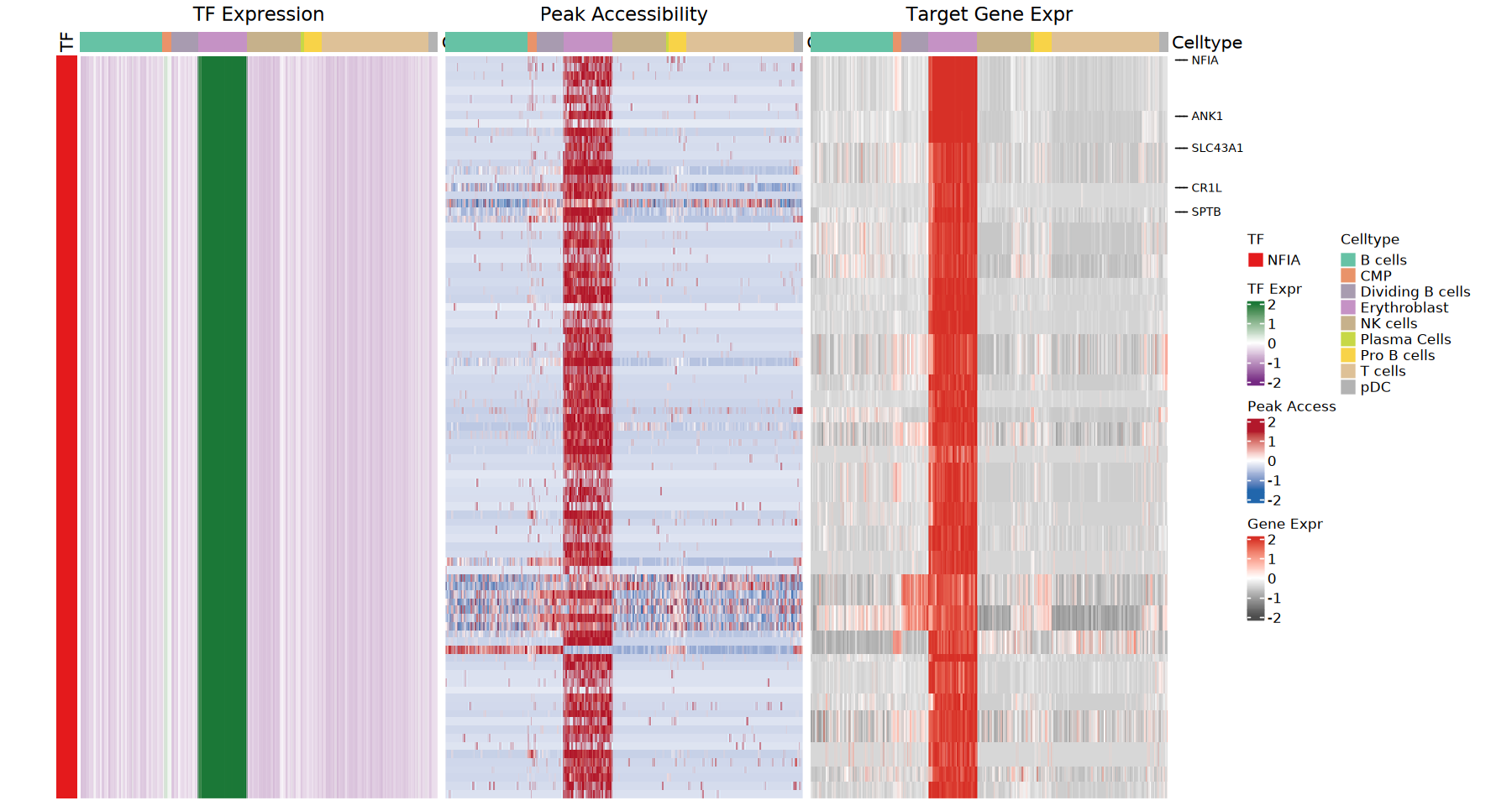

💡 Note:
In the final heatmap, trace the signal propagation horizontally. For a genuine and active positive regulatory trio, you will observe marked "cross-modal co-variation": in a specific cell population, up-regulation of the TF's expression (high signal in the left panel) drives increased chromatin accessibility at its corresponding binding Peak (high signal in the middle panel), ultimately leading to transcriptional activation of the downstream core target gene cohort (high signal in the right panel).

6.3 Subpopulation-Specific Expression Heatmap of Core TF Target Gene Modules

In the global multi-omics co-variation heatmap (Section 5.3, actually 6.2), we validated the cis-regulatory relationships among TFs, Peaks, and Targets. Next, we need to further verify whether these target gene modules driven by the core TFs truly determine cellular heterogeneity and classification.

The code in this section extracts each of the Top 10 core transcription factors locked in the preceding analysis and specifically plots an expression heatmap of their dedicated target gene cohorts across cell subpopulations.

Data Processing and Visualization Logic:

Target Gene Extraction and Matrix Projection: For each TF of interest, extract its top strongly driven target genes (controlled by the top_n_genes_per_tf_heatmap parameter) based on linkage_score. Then precisely extract the expression profiles of these target genes across all valid cells from the single-cell transcriptome matrix.
Subpopulation-Based Matrix Aggregation (Matrix Multiplication): To eliminate single-cell sparse noise and accentuate macroscopic differences between cell groups, the code builds a model matrix (model.matrix) and uses efficient matrix multiplication to compute the mean expression of each target gene in each cell subpopulation.
Feature Standardization and Two-Way Clustering: The aggregated mean matrix is row-wise Z-score standardized. When plotting, both row (gene) and column (cell group) unsupervised hierarchical clustering are enabled.

plot_tf_targets_heatmap <- function(tf_name, trios_df, seurat_obj, celltype_col = "shoudong", output_dir = NULL, top_n_genes = top_n_genes_per_tf_heatmap) { 
  targets <- trios_df %>% 
    filter(TF == tf_name) %>% 
    dplyr::select(gene, linkage_score) %>% 
    distinct() %>% 
    arrange(desc(linkage_score)) 
  
  if (nrow(targets) == 0) { 
    return(NULL) 
  } 
  
  if (nrow(targets) > top_n_genes) { 
    plot_genes <- targets$gene[1:top_n_genes] 
  } else { 
    plot_genes <- targets$gene 
  } 
  
  if (!celltype_col %in% colnames(seurat_obj@meta.data)) { 
    if ("seurat_clusters" %in% colnames(seurat_obj@meta.data)) { 
      celltype_col <- "seurat_clusters" 
    } else { 
      celltype_col <- "ident" 
    } 
  } 
  
  expr_data <- tryCatch({ 
    GetAssayData(seurat_obj, assay = "RNA", layer = "data") 
  }, error = function(e) { 
    GetAssayData(seurat_obj, assay = "RNA", slot = "data") 
  }) 
  
  valid_genes <- intersect(plot_genes, rownames(expr_data)) 
  if (length(valid_genes) < 2) { 
    return(NULL) 
  } 
  
  idents <- seurat_obj@meta.data[[celltype_col]] 
  if (is.null(idents)) idents <- Idents(seurat_obj) 
  
  valid_cells <- !is.na(idents) 
  expr_subset <- expr_data[valid_genes, valid_cells, drop=FALSE] 
  idents_subset <- idents[valid_cells] 
  
  mm <- model.matrix(~ 0 + factor(idents_subset)) 
  colnames(mm) <- levels(factor(idents_subset)) 
  mat_sum <- expr_subset %*% mm 
  mat_count <- colSums(mm) 
  mat_avg <- t(t(mat_sum) / mat_count) 
  
  mat_scale <- t(scale(t(mat_avg))) 
  col_fun <- colorRamp2(c(-2, 0, 2), c("#440154FF", "#21908CFF", "#FDE725FF")) 
  
  celltypes <- colnames(mat_scale) 
  ct_colors <- suppressWarnings(colorRampPalette(RColorBrewer::brewer.pal(8, "Set2"))(length(celltypes)))
  names(ct_colors) <- celltypes 
  
  ha_bottom <- HeatmapAnnotation( 
    Celltype = celltypes, 
    col = list(Celltype = ct_colors), 
    show_legend = TRUE, 
    show_annotation_name = TRUE 
  ) 
  
  ht <- Heatmap(mat_scale, 
                name = "Z-score", 
               # col = col_fun, 
                col = col_peak, 
                cluster_rows = TRUE, 
                show_row_names = FALSE, 
                row_title = paste0("Target Genes (n=", length(valid_genes), ")"), 
                cluster_columns = TRUE, 
                show_column_names = TRUE, 
                column_names_rot = 90,
                show_column_dend = FALSE,
                show_row_dend = FALSE,
                column_title = paste0("Expression in ", tf_name, " Trios"), 
                bottom_annotation = ha_bottom, 
                use_raster = TRUE 
  ) 
  
  if (!is.null(output_dir)) { 
    dir.create(output_dir, recursive = TRUE, showWarnings = FALSE) 
    filename <- file.path(output_dir, paste0(tf_name, "_targets_heatmap.pdf")) 
    pdf(filename, width = 8, height = 4) 
    draw(ht) 
    dev.off() 
  } 
  
  return(ht)
}

dir.create(heatmap_out_dir, recursive = TRUE, showWarnings = FALSE)

save_and_encode_heatmap <- function(ht, filename_base, width = 8, height = 4) {
  full_path_pdf <- paste0(filename_base, ".pdf")
  temp_png <- tempfile(fileext = ".png")

  pdf(full_path_pdf, width = width, height = height)
  draw(ht)
  invisible(dev.off())

  png(temp_png, width = width * 100, height = height * 100, res = 100)
  draw(ht)
  invisible(dev.off())
  return(NULL)
}

plot_list <- list()
for (tf in top_10_tfs) { 
  ht <- tryCatch({ 
    plot_tf_targets_heatmap(tf, trios_df, seurat_obj = data, celltype_col = celltype_col, output_dir = NULL, top_n_genes = top_n_genes_per_tf_heatmap) 
  }, error = function(e) { 
    return(NULL)
  }) 
  
  if (!is.null(ht)) {
    file_base <- file.path(heatmap_out_dir, paste0(tf, "_targets_heatmap"))
    res <- save_and_encode_heatmap(ht, file_base)
  }
}

ht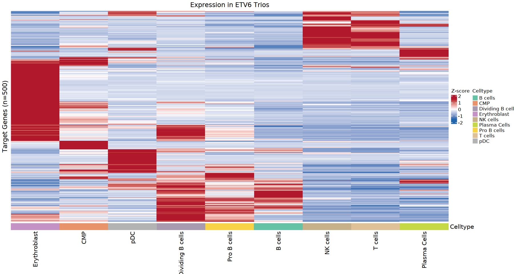

💡 Note: The example shows the expression of target genes regulated by one of the TFs across different cell types; please refer to the ./result directory for the complete results.
Column Clustering Validation: Inspect the dendrogram at the top of the heatmap. If the TF is a master regulator of a given cell lineage, you will see that the expression pattern of its target gene cohort perfectly separates that target cell population from other cell populations (forming an independent branch).
Gene Co-Expression Modules: Looking vertically, dark-red (high Z-score) blocks represent the downstream gene network that the TF concentrates on activating in a specific cellular state — providing a direct list of targets for subsequent fine-grained characterization of cellular-state molecular signatures.

6.4 TF–Target Regulatory Network Graph

To intuitively parse the radial regulatory topology of transcription factors, the code in this section uses igraph to construct and draw a star-shaped regulatory network centered on a core TF.

Biological Logic and Network Mapping Rules:

Node Filtering and Mapping:
- Node Selection: Not all high-scoring target genes are plotted. The code computes the average expression level (AverageExpression) of all target genes across the entire cell population and filters out extremely lowly expressed background genes (controlled by the min_expr_percentile parameter). This ensures that targets in the network not only possess regulatory potential but also have genuine transcriptional activity in the current tissue.
- Node Size: The physical area of a node is strictly mapped from the gene's log-transformed mean expression (log1p(expression)). The larger the node, the higher the baseline transcriptional activity of that gene in the cellular system.
- Node Color: The central transcription factor (TF) is fixed as a striking orange (hub node) to highlight its network-hub status.
Physical and Statistical Mapping of Edges:
- Edge Width: Line thickness is mapped directly from the Linkage Score of the regulatory pair. The thicker the line, the stronger the multi-omics evidence (TF binding affinity and Peak accessibility) supporting that regulatory axis.
- Edge Color: Strictly reflects the directionality of regulation. Red lines represent positive correlation, indicating transcriptional activation by the TF on the target; blue lines represent negative correlation, indicating transcriptional repression.
Topological Layout: The Fruchterman–Reingold (FR) force-directed layout algorithm (layout_with_fr) is used. This algorithm automatically adjusts node distances according to edge weights, physically "pulling" the core target genes with the tightest and strongest associations toward the network center, thereby clearly presenting the hierarchical regulatory structure from core to periphery.

options(warn = -1)
plot_tf_network <- function(tf_name, trios_df, seurat_obj, output_dir = NULL, 
                            min_expr_percentile = 0.2, 
                            max_nodes = 50) {          

  target_data <- trios_df %>% 
    filter(TF == tf_name) %>% 
    mutate(correlation = if("tf_gene_cor" %in% names(.)) tf_gene_cor else peak_gene_cor) %>% 
    group_by(gene) %>% 
    summarize( 
      linkage_score = max(linkage_score, na.rm = TRUE), 
      correlation = mean(correlation, na.rm = TRUE),    
      .groups = "drop" 
    ) %>% 
    arrange(desc(linkage_score)) 
  
  if (nrow(target_data) == 0) return(NULL) 
  
  all_genes <- rownames(GetAssayData(seurat_obj, assay = "RNA")) 
  valid_features <- intersect(c(tf_name, target_data$gene), all_genes) 
  
  if (length(valid_features) == 0) return(NULL) 
  
  avg_expr_list <- AverageExpression(seurat_obj, features = valid_features, assay = "RNA") 
  if ("RNA" %in% names(avg_expr_list)) { 
    avg_expr <- avg_expr_list$RNA 
  } else { 
    avg_expr <- avg_expr_list[[1]] 
  } 
  
  if (is.null(avg_expr) || nrow(avg_expr) == 0) { 
     gene_expr_vals <- setNames(rep(0, length(valid_features)), valid_features) 
  } else { 
     gene_expr_vals <- rowMeans(avg_expr) 
  } 
  
  get_expr <- function(genes, expr_vec) { 
    vals <- expr_vec[genes] 
    vals[is.na(vals)] <- 0 
    return(vals) 
  } 
  target_data$expression <- get_expr(target_data$gene, gene_expr_vals) 

  if (max(target_data$expression) > 0) { 
      expr_threshold <- quantile(target_data$expression[target_data$expression > 0], min_expr_percentile, na.rm = TRUE) 
      target_data_filtered <- target_data %>% filter(expression >= expr_threshold) 
  } else { 
      target_data_filtered <- target_data 
  } 
  
  if (nrow(target_data_filtered) > max_nodes) { 
    target_data_filtered <- head(target_data_filtered, max_nodes) 
  } 
  
  if (nrow(target_data_filtered) == 0) return(NULL) 
  

  tf_expr_val <- get_expr(tf_name, gene_expr_vals) 
  if (tf_expr_val == 0 && nrow(target_data_filtered) > 0) tf_expr_val <- max(target_data_filtered$expression) 
   
  target_cors <- target_data_filtered$correlation 
  target_cors[is.na(target_cors)] <- 0 
  
  nodes_df <- data.frame( 
    id = c(tf_name, target_data_filtered$gene), 
    type = c("TF", rep("Target", nrow(target_data_filtered))), 
    expression = c(tf_expr_val, target_data_filtered$expression), 
    correlation = c(0, target_cors), 
    stringsAsFactors = FALSE 
  ) 
  
   edge_colors <- ifelse(target_data_filtered$correlation > 0, "#b2182b", "#2166ac") 
   edges_df <- data.frame( 
     from = tf_name, 
     to = target_data_filtered$gene, 
     weight = target_data_filtered$linkage_score, 
     color = edge_colors 
   ) 
   
   g <- graph_from_data_frame(d = edges_df, vertices = nodes_df, directed = TRUE) 

   expr_scaled <- log1p(V(g)$expression) 
  
  if (max(expr_scaled) == min(expr_scaled)) { 
      size_vec <- rep(10, length(expr_scaled)) 
  } else { 
      size_vec <- scales::rescale(expr_scaled, to = c(5, 15)) 
  } 

  V(g)$size <- size_vec 
  V(g)$size[V(g)$type == "TF"] <- 25 
  
  color_vec <- rep("#2166ac", vcount(g))
  color_vec[V(g)$correlation > 0] <- "#b2182b"
  color_vec[V(g)$type == "TF"] <- "#FDB462"
  V(g)$color <- adjustcolor(color_vec, alpha.f = 0.8) 
  
  if (max(E(g)$weight) == min(E(g)$weight)) { 
      E(g)$width <- 1.5 
  } else { 
      E(g)$width <- scales::rescale(E(g)$weight, to = c(0.5, 3)) 
  } 
  E(g)$arrow.size <- 0.3
  E(g)$curved <- 0.2 
  
  V(g)$label <- V(g)$name 
  V(g)$label.color <- "black" 
  V(g)$label.cex <- ifelse(V(g)$type == "TF", 1.2, 0.7)
  V(g)$label.font <- 2 
  
  l <- layout_with_fr(g) 
  
  if (!is.null(output_dir)) { 
    dir.create(output_dir, recursive = TRUE, showWarnings = FALSE) 
    filename <- file.path(output_dir, paste0(tf_name, "_network.pdf")) 
    pdf(filename, width = 8, height = 8) 
    plot(g, layout = l, main = paste0(tf_name, " Network"), vertex.frame.color = "white", margin = c(0,0,0,0)) 
    legend("bottomright", legend = c("TF", "Pos Cor", "Neg Cor"), col = c("#FDB462", "#b2182b", "#2166ac"), pch = 19, pt.cex = 1.5, bty = "n") 
    dev.off() 
  } 
  
  return(list(g = g, layout = l))
}

dir.create(network_out_dir, recursive = TRUE, showWarnings = FALSE)

save_and_encode_network <- function(g, layout, filename_base, width = 8, height = 8) {
  full_path_pdf <- paste0(filename_base, ".pdf")
  temp_png <- tempfile(fileext = ".png")

  pdf(full_path_pdf, width = width, height = height)
  plot(g, layout = layout, vertex.frame.color = "white", margin = c(0,0,0,0))
  legend("bottomright", legend = c("TF", "Pos Cor", "Neg Cor"), col = c("#FDB462", "#b2182b", "#2166ac"), pch = 19, pt.cex = 1.5, bty = "n")
  invisible(dev.off())

  png(temp_png, width = width * 100, height = height * 100, res = 100)
  plot(g, layout = layout, vertex.frame.color = "white", margin = c(0,0,0,0))
  legend("bottomright", legend = c("TF", "Pos Cor", "Neg Cor"), col = c("#FDB462", "#b2182b", "#2166ac"), pch = 19, pt.cex = 1.5, bty = "n")
  invisible(dev.off())
  return(NULL)
}

plot_list <- list()

for (tf in top_10_tfs) {

  res_obj <- tryCatch({
    plot_tf_network(tf, trios_df, seurat_obj = data, output_dir = NULL, max_nodes = network_max_nodes)
  }, error = function(e) return(NULL))
  
  if (!is.null(res_obj)) {
    file_base <- file.path(network_out_dir, paste0(tf, "_network"))
    res_img <- save_and_encode_network(res_obj$g, res_obj$layout, file_base)
  }
}
options(warn = 0)

 plot(res_obj$g, layout = res_obj$layout, vertex.frame.color = "white", margin = c(0,0,0,0))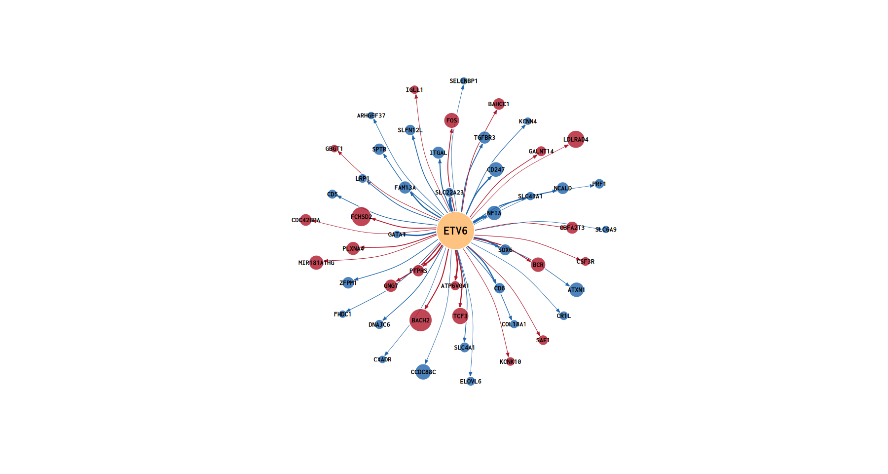

💡 Note: When inspecting the generated star-shaped network, pay particular attention to the genes that are closest to the central orange TF and have the largest node area. These genes are not only under strong physical driving force from the TF (thickest lines), but are also themselves highly transcriptionally active (largest nodes) — they are typically the key effectors mediating the core biological functions downstream of that TF. Furthermore, the ratio of red to blue lines allows quick assessment of whether the TF behaves as a global transcriptional activator or repressor in the current cellular state.

6.5 Global Multi-TF Cooperative Regulatory Network (Global Regulatory Network)

In the single-TF network (Section 6.4), only a "one-to-many" star-shaped structure is visible. However, in real biological systems, core transcription factors often engage in dense co-regulation and cross-talk.

The code in this section uses igraph together with a customized geometric topology algorithm to construct a global regulatory network integrating multiple core TFs. It reveals not only the sphere of influence of individual TFs, but also intuitively exposes the shared target gene modules across transcription factors.

Core Topology Algorithm and Biological Mapping Rules:

Core Hub Extraction and Expression Mapping:
- Based on Total Linkage Score, extract the Top TFs (e.g., Top 20) with the highest regulatory weight in the current cellular system.
- Node physical size is strictly mapped from their mean expression in scRNA-seq (log1p(expression)).
- The display scale of core TFs is dynamically adjusted based on network degree (i.e., number of incident edges): TFs with higher degree appear larger, intuitively highlighting their status as Master Regulators in the global network.
Module Detection and Louvain Clustering (Community Detection):
- After constructing the undirected network, the code internally invokes the cluster_louvain algorithm (a community detection algorithm based on modularity optimization).
- This step runs silently in the background; by tracing edge weights (Linkage Score), it partitions the entire large network into multiple tightly interacting sub-modules (Modules), and outputs the results to the All_TFs_network_modules.txt file, providing a data foundation for subsequent extraction of specific biological pathway gene sets.
Customized Circular and Radial Topological Layout (Geometric Layout):
- Core TF Ring: All hub TFs are forcibly distributed evenly along an inner ring, ensuring that core hubs are not overwhelmed by the multitude of target genes.
- Shared Targets: Target genes regulated by two or more TFs (out-degree > 1) have their coordinates precisely computed via vector mean and placed in the angular inner ring between the corresponding TFs. These nodes represent key cross-talk hubs.
- Unique Targets: Dedicated target genes regulated by only a single TF are arranged radially in the outer layer around that TF via tangent vector computation.

plot_all_tf_network <- function(trios_df, seurat_obj, output_dir = NULL,
                                max_tfs = 20,
                                max_targets_per_tf = 50,
                                min_expr_percentile = 0.2,
                                detect_modules = TRUE,
                                tf_ring_expand = 1.35,
                                shared_target_inner_shrink = 0.72,
                                unique_target_outer_expand = 0.22,
                                shared_target_spread = 0.12,
                                max_target_labels = Inf) {
  edge_df <- trios_df %>%
    mutate(correlation = if ("tf_gene_cor" %in% names(.)) tf_gene_cor else peak_gene_cor) %>%
    group_by(TF, gene) %>%
    summarize(
      linkage_score = max(linkage_score, na.rm = TRUE),
      correlation = mean(correlation, na.rm = TRUE),
      .groups = "drop"
    )

  tf_rank <- edge_df %>%
    group_by(TF) %>%
    summarize(total_linkage = sum(linkage_score, na.rm = TRUE), .groups = "drop") %>%
    arrange(desc(total_linkage)) %>%
    head(max_tfs) %>%
    pull(TF)

  edge_df <- edge_df %>%
    filter(TF %in% tf_rank) %>%
    group_by(TF) %>%
    arrange(desc(linkage_score), .by_group = TRUE) %>%
    slice_head(n = max_targets_per_tf) %>%
    ungroup()

  if (nrow(edge_df) == 0) return(NULL)

  all_genes <- rownames(GetAssayData(seurat_obj, assay = "RNA"))
  features <- intersect(unique(c(edge_df$TF, edge_df$gene)), all_genes)
  if (length(features) == 0) return(NULL)

  avg_expr_list <- AverageExpression(seurat_obj, features = features, assay = "RNA")
  avg_expr <- if ("RNA" %in% names(avg_expr_list)) avg_expr_list$RNA else avg_expr_list[[1]]
  expr_vec <- if (is.null(avg_expr) || nrow(avg_expr) == 0) {
    setNames(rep(0, length(features)), features)
  } else {
    rowMeans(avg_expr)
  }

  edge_df$target_expr <- expr_vec[edge_df$gene]
  edge_df$target_expr[is.na(edge_df$target_expr)] <- 0

  if (max(edge_df$target_expr) > 0) {
    expr_cut <- quantile(edge_df$target_expr[edge_df$target_expr > 0], min_expr_percentile, na.rm = TRUE)
    edge_df <- edge_df %>% filter(target_expr >= expr_cut)
  }

  if (nrow(edge_df) == 0) return(NULL)

  target_stat <- edge_df %>%
    group_by(gene) %>%
    summarize(
      expression = max(target_expr, na.rm = TRUE),
      cor_mean = mean(correlation, na.rm = TRUE),
      .groups = "drop"
    )

  tf_stat <- edge_df %>%
    group_by(TF) %>%
    summarize(
      expression = ifelse(TF[1] %in% names(expr_vec), expr_vec[TF[1]], 0),
      degree_like = n(),
      .groups = "drop"
    )

  nodes_tf <- data.frame(
    name = tf_stat$TF,
    type = "TF",
    expression = tf_stat$expression,
    cor_mean = 0,
    degree_like = tf_stat$degree_like,
    stringsAsFactors = FALSE
  )

  nodes_target <- data.frame(
    name = target_stat$gene,
    type = "Target",
    expression = target_stat$expression,
    cor_mean = target_stat$cor_mean,
    degree_like = 0,
    stringsAsFactors = FALSE
  )

  nodes <- bind_rows(nodes_tf, nodes_target) %>%
    group_by(name) %>%
    summarize(
      type = ifelse(any(type == "TF"), "TF", "Target"),
      expression = max(expression, na.rm = TRUE),
      cor_mean = mean(cor_mean, na.rm = TRUE),
      degree_like = max(degree_like, na.rm = TRUE),
      .groups = "drop"
    )

  edge_colors <- ifelse(edge_df$correlation > 0, "#d73027", "#4575b4")
  edges <- data.frame(
    from = edge_df$TF,
    to = edge_df$gene,
    weight = edge_df$linkage_score,
    color = edge_colors,
    stringsAsFactors = FALSE
  )

  g <- igraph::graph_from_data_frame(edges, vertices = nodes, directed = TRUE)

  if (detect_modules && vcount(g) > 2 && ecount(g) > 0) {
    g_mod <- igraph::as.undirected(
      igraph::simplify(g, remove.multiple = TRUE, remove.loops = TRUE,
                       edge.attr.comb = list(weight = "sum", color = "first")),
      mode = "collapse",
      edge.attr.comb = list(weight = "sum", color = "first")
    )
    if (ecount(g_mod) > 0) {
      cl <- igraph::cluster_louvain(g_mod, weights = E(g_mod)$weight)
      mod_map <- igraph::membership(cl)
      V(g)$module_id <- as.integer(mod_map[V(g)$name])
    } else {
      V(g)$module_id <- rep(1L, vcount(g))
    }
  } else {
    V(g)$module_id <- rep(1L, vcount(g))
  }

  v_type <- V(g)$type
  v_expr <- V(g)$expression
  v_deg <- igraph::degree(g, mode = "all")

  tf_idx <- which(v_type == "TF")
  tg_idx <- which(v_type == "Target")

  size_vec <- rep(5, vcount(g))
  if (length(tf_idx) > 0) {
    tf_deg <- v_deg[tf_idx]
    size_vec[tf_idx] <- if (max(tf_deg) == min(tf_deg)) 11 else scales::rescale(tf_deg, to = c(8.5, 14.5))
  }
  if (length(tg_idx) > 0) {
    tg_expr <- log1p(v_expr[tg_idx])
    size_vec[tg_idx] <- if (max(tg_expr) == min(tg_expr)) 6 else scales::rescale(tg_expr, to = c(3.5, 9))
  }
  V(g)$size <- size_vec

  color_vec <- rep("#9e9e9e", vcount(g))
  if (length(tg_idx) > 0) {
    tg_cor <- V(g)$cor_mean[tg_idx]
    tg_cor[is.na(tg_cor)] <- 0
    color_vec[tg_idx] <- ifelse(tg_cor > 0, "#d73027", "#4575b4")
  }
  if (length(tf_idx) > 0) color_vec[tf_idx] <- "#FDB462"
  V(g)$color <- adjustcolor(color_vec, alpha.f = 0.85)

  w <- E(g)$weight
  E(g)$width <- if (max(w) == min(w)) 1.2 else scales::rescale(w, to = c(0.3, 2.5))
  E(g)$color <- adjustcolor(E(g)$color, alpha.f = 0.5)

  label_vec <- rep("", vcount(g))
  if (length(tf_idx) > 0) label_vec[tf_idx] <- V(g)$name[tf_idx]
  if (length(tg_idx) > 0) {
    target_label_n <- if (is.infinite(max_target_labels)) length(tg_idx) else min(as.integer(max_target_labels), length(tg_idx))
    if (target_label_n > 0) {
      tg_keep <- tg_idx[order(v_deg[tg_idx], decreasing = TRUE)][seq_len(target_label_n)]
      label_vec[tg_keep] <- V(g)$name[tg_keep]
    }
  }
  V(g)$label <- label_vec
  V(g)$label.color <- "black"
  V(g)$label.cex <- ifelse(V(g)$type == "TF", 0.82, 0.42)
  V(g)$label.font <- 2

  edge_w <- E(g)$weight
  edge_w[is.na(edge_w)] <- median(edge_w, na.rm = TRUE)
  edge_w <- pmax(edge_w, quantile(edge_w, 0.05, na.rm = TRUE))
  lay <- igraph::layout_with_fr(g, niter = 2800, weights = edge_w)

  if (length(tf_idx) > 2) {
    ctr <- colMeans(lay)
    d <- sqrt((lay[, 1] - ctr[1])^2 + (lay[, 2] - ctr[2])^2)
    r <- as.numeric(stats::quantile(d, 0.78, na.rm = TRUE)) * tf_ring_expand
    tf_order <- tf_idx[order(v_deg[tf_idx], decreasing = TRUE)]
    theta <- seq(0, 2 * pi, length.out = length(tf_order) + 1)[-1]
    ring <- cbind(ctr[1] + r * cos(theta), ctr[2] + r * sin(theta))
    lay[tf_order, ] <- ring

    tg_in_deg <- igraph::degree(g, v = tg_idx, mode = "in")
    shared_tg_idx <- tg_idx[tg_in_deg > 1]
    unique_tg_idx <- tg_idx[tg_in_deg <= 1]

    if (length(shared_tg_idx) > 0) {
      mean_angle <- rep(0, length(shared_tg_idx))
      for (i in seq_along(shared_tg_idx)) {
        nb <- as.integer(igraph::neighbors(g, shared_tg_idx[i], mode = "in"))
        if (length(nb) > 0) {
          pv <- lay[nb, , drop = FALSE] - matrix(ctr, nrow = length(nb), ncol = 2, byrow = TRUE)
          mv <- colMeans(pv)
          mean_angle[i] <- atan2(mv[2], mv[1])
        }
      }
      ord <- order(mean_angle)
      n_shared <- length(shared_tg_idx)
      base_r <- r * shared_target_inner_shrink
      slot_angle <- if (n_shared > 1) (2 * pi / n_shared) else 0
      for (k in seq_along(ord)) {
        idx <- shared_tg_idx[ord[k]]
        ring_id <- ((k - 1) %% 3) + 1
        ring_scale <- 1 + (ring_id - 2) * shared_target_spread
        ang_shift <- (floor((k - 1) / 3) - floor((n_shared - 1) / 6)) * slot_angle * 0.35
        ang <- mean_angle[ord[k]] + ang_shift
        rr <- base_r * ring_scale
        lay[idx, ] <- c(ctr[1] + rr * cos(ang), ctr[2] + rr * sin(ang))
      }
    }

    if (length(unique_tg_idx) > 0) {
      parent_tf <- rep(NA_character_, length(unique_tg_idx))
      for (i in seq_along(unique_tg_idx)) {
        nb <- igraph::neighbors(g, unique_tg_idx[i], mode = "in")
        if (length(nb) > 0) parent_tf[i] <- V(g)$name[as.integer(nb)[1]]
      }

      valid <- !is.na(parent_tf)
      unique_tg_idx <- unique_tg_idx[valid]
      parent_tf <- parent_tf[valid]

      if (length(unique_tg_idx) > 0) {
        for (tf_name in unique(parent_tf)) {
          ids <- unique_tg_idx[parent_tf == tf_name]
          tf_node <- which(V(g)$name == tf_name)
          if (length(tf_node) == 0) next

          tf_pos <- lay[tf_node[1], ]
          v <- tf_pos - ctr
          vn <- sqrt(sum(v^2))
          if (vn == 0) {
            out_u <- c(1, 0)
          } else {
            out_u <- v / vn
          }
          tan_u <- c(-out_u[2], out_u[1])
          offsets <- seq(-(length(ids) - 1) / 2, (length(ids) - 1) / 2, length.out = length(ids))

          for (k in seq_along(ids)) {
            lay[ids[k], ] <- tf_pos + out_u * (unique_target_outer_expand * r) + tan_u * (offsets[k] * 0.06 * r)
          }
        }
      }
    }
  }

  if (!is.null(output_dir)) {
    dir.create(output_dir, recursive = TRUE, showWarnings = FALSE)
    module_df <- data.frame(
      node = V(g)$name,
      type = V(g)$type,
      module_id = V(g)$module_id,
      stringsAsFactors = FALSE
    )
    write.table(
      module_df,
      file = file.path(output_dir, "All_TFs_network_modules.txt"),
      sep = "\t",
      quote = FALSE,
      row.names = FALSE
    )
    fn <- file.path(output_dir, "All_TFs_network.pdf")
    pdf(fn, width = 9, height = 9)
    old_par <- par(no.readonly = TRUE)
    on.exit(par(old_par), add = TRUE)
    par(mar = c(0.8, 0.8, 2.0, 0.8))

    plot(
      g,
      layout = lay,
      main = "",
      vertex.frame.color = "white",
      edge.arrow.size = 0.12,
      margin = 0,
      rescale = TRUE
    )
    title(main = "Global TF-Target Regulatory Network", line = 0.4, cex.main = 1.2)
    legend(
      "topleft",
      inset = c(0.02, 0.02),
      legend = c("TF", "Target(+)", "Target(-)"),
      col = c("#FDB462", "#d73027", "#4575b4"),
      pch = 19,
      pt.cex = 1.3,
      bty = "n",
      title = "Node Type"
    )
    dev.off()
    fn_png <- file.path(output_dir, "All_TFs_network.png") 
    png(fn_png, width = 9, height = 9, units = "in", res = 300) 
    par(mar = c(0.8, 0.8, 2.0, 0.8)) 
    
    plot( 
      g, 
      layout = lay, 
      main = "", 
      vertex.frame.color = "white", 
      edge.arrow.size = 0.12, 
      margin = 0, 
      rescale = TRUE 
    ) 
    title(main = "Global TF-Target Regulatory Network", line = 0.4, cex.main = 1.2) 
    legend( 
      "topleft", 
      inset = c(0.02, 0.02), 
      legend = c("TF", "Target(+)", "Target(-)"), 
      col = c("#FDB462", "#d73027", "#4575b4"), 
      pch = 19, 
      pt.cex = 1.3, 
      bty = "n", 
      title = "Node Type" 
    ) 
    dev.off()   
  }

  list(
    g = g,
    layout = lay,
    module_df = data.frame(
      node = V(g)$name,
      type = V(g)$type,
      module_id = V(g)$module_id,
      stringsAsFactors = FALSE
    ),
    module_sizes = sort(table(V(g)$module_id), decreasing = TRUE)
  )
}

network_res <- tryCatch({
  plot_all_tf_network(
    trios_df = trios_df,
    seurat_obj = data,
    output_dir = network_out_dir,
    max_tfs = global_network_max_tfs,
    max_targets_per_tf = global_network_max_targets_per_tf
  )
}, error = function(e) {
  print(paste("warnning:", e$message))
  NULL
})

💡 Note: In the generated global network, focus on the inner "shared target cohort." These nodes, connected to by multiple TFs, are often the "bottleneck genes" that maintain tissue homeostasis or drive specific biological processes. The radially arranged peripheral genes, by contrast, represent each TF's dedicated arsenal for maintaining cell-type-specific functions.

old_par <- par(no.readonly = TRUE)
par(mar = c(0, 0, 0, 0))
  
plot(
    network_res$g, 
    layout = network_res$layout, 
    main = "", 
    vertex.frame.color = "white", 
    edge.arrow.size = 0.12, 
    margin = 0, 
    rescale = TRUE
  )
title(main = "Global TF-Target Regulatory Network", line = 0.4, cex.main = 1.2)
legend(
    "topleft", 
    inset = c(0.02, 0.02), 
    legend = c("TF", "Target(+)", "Target(-)"), 
    col = c("#FDB462", "#d73027", "#4575b4"), 
    pch = 19, 
    pt.cex = 1.3, 
    bty = "n", 
    title = "Node Type"
)
  
par(old_par)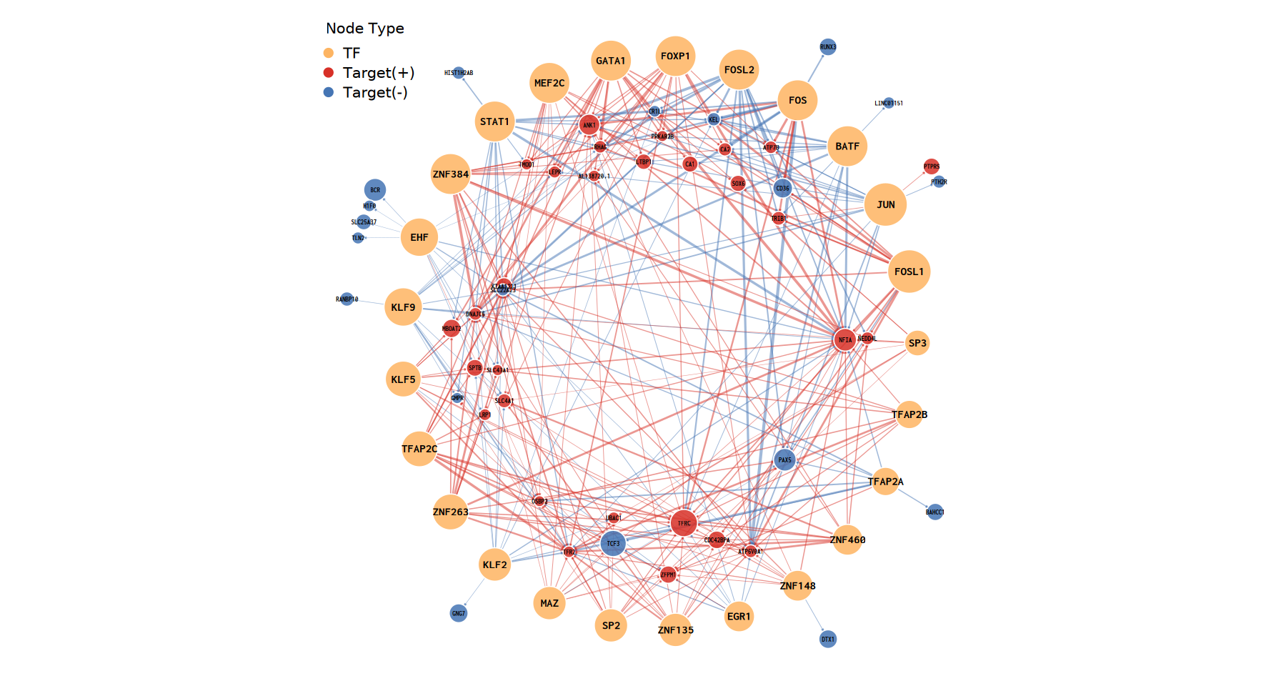

💡 Note: In the generated global network, focus your attention on the inner region interwoven with lines from multiple TFs. These tightly encircled "shared targets" are typically the "bottleneck genes" that maintain tissue homeostasis or sit at the chokepoint of a key signaling pathway. Genes scattered along the outer radial periphery, on the other hand, more often represent the "dedicated arsenal" that individual TFs mobilize to maintain the characteristics of a specific cell subpopulation. In addition, observing the density of connections among core TFs can help you identify which transcription factors are "clustering together" to exert cooperative regulation.

ATAC + RNA Multi-omics: Trios Analysis ​

1. Tutorial Overview ​

2. Input File Preparation ​

3. Initial Trio Assembly ​

3.1 Loading the Peak2Gene Result File (Gene2PeakLinks.xls) ​

3.2 Loading Multi-Omics Data and Motif–Peak Spatial Mapping ​

3.3 Completing Initial Trio Assembly and Background Noise Filtering ​

4. Active Regulatory Filtering and Statistical Testing ​

4.1 Computing TF–Target Gene Expression Correlation (TF–Gene Correlation) ​

4.2 Computing Consistency Correlation between TF Activity and Its Own Expression ​

4.3 Computing Correlation between TF Activity and Target Gene Expression (Distinguishing Activation from Repression) ​

4.4 Composite Regulatory Strength Score (Linkage Score Computation) ​

5. Trios Filtering and High-Confidence Network Output ​

6. Trios Visualization ​

6.1 Core TF Selection and Target Gene Regulatory Scatter Plot ​

6.2 Trios Regulatory Co-Variation Heatmap ​

6.3 Subpopulation-Specific Expression Heatmap of Core TF Target Gene Modules ​

6.4 TF–Target Regulatory Network Graph ​

6.5 Global Multi-TF Cooperative Regulatory Network (Global Regulatory Network) ​