ATAC + RNA 多组学：Trios 分析

作者: SeekGene

时长: 69 分钟

字数: 16.2k 字

更新: 2026-07-07

阅读: 0 次

1. 教程简介

本教程基于 SeekArc 单细胞多组学数据（scRNA-seq + scATAC-seq），旨在揭示细胞状态特异性基因表达程序背后的转录调控逻辑。TF–Peak–Gene 三元组是解析该调控网络的核心功能单元：

TF（调控发起者）：转录因子通过识别并结合靶 DNA 上的特征性基序（Motif），发起特异性调控。
Peak（调控媒介）：代表染色质开放区域，常富集于增强子、启动子等顺式调控元件；其可及性是 TF 发挥功能的物理前提。
Gene（功能输出）：基因表达变化是上游调控事件在转录层面的最终体现。

本教程的核心目标是：在特定细胞状态下，系统识别哪些 TF 通过结合哪些调控 Peak，最终调控了哪些 Gene，从而重建具有生物学解释力的调控逻辑链条。

suppressPackageStartupMessages(suppressWarnings({
    library(presto)
    library(ggrepel)
    library(Seurat)
    library(BiocGenerics)
    library(S4Vectors)
    library(IRanges)
    library(Signac)
    library(ComplexHeatmap)
    library(RColorBrewer)
    library(GenomicRanges)
    library(igraph)
    library(Biobase)
    library(AnnotationDbi)
    library(org.Hs.eg.db)
    #library(org.Mm.eg.db)
    library(JASPAR2020)
    library(TFBSTools)
    library(memuse)
    library(stringr)
    library(dplyr)
    library(DOSE)
    library(clusterProfiler)
    library(enrichplot)
    library(foreach)
    library(doParallel)
    library(circlize)
}))

2. 输入文件准备

首先，配置并行计算参数与文件路径。我们需要提供以下结果文件：

Gene2PeakLinks.xls：Peak-to-Gene（P2G）分析结果。
output.rds：包含单细胞 RNA 和 ATAC 多模态数据及 Motif 注释的 Seurat 对象。

## species：物种信息，"human" 或 "mouse" 等，用于 TF 命名大小写转换及下游富集分析
species = "human"

## links_path：Peak2Gene 模块输出的 Gene2PeakLinks.xls 文件路径，包含 Peak 与 Gene 的相关性链接
links_path = "/path/to/Gene2PeakLinks.xls"

## rds_path：输入的 Seurat 对象 RDS 文件路径，包含已预处理的单细胞多组学数据及 Motif 注释
rds_path = "/path/to/output.rds"

## pseudobulk_size：拟 bulk 大小，表示每组聚合多少个细胞用于计算相关性（建议：10；设为 1 则不启用）
pseudobulk_size = 10

## min_motif_score：最小 Motif Score 阈值，用于过滤低亲和力的 TF-Peak 结合（建议：10.0；设为 0 则不过滤）
min_motif_score = 10.0

## min_tf_gene_cor：最小 TF-Gene 表达相关性绝对值阈值，用于筛选表达水平上具有共变性的 TF-靶基因对（建议：0.2）
min_tf_gene_cor = 0.2

## min_tf_activity_cor：最小 TF 活性-表达一致性相关性绝对值阈值（建议：0.2）
min_tf_activity_cor = 0.2

## min_tf_activity_target_cor：最小 TF 活性-靶基因表达相关性绝对值阈值（建议：0.2）
min_tf_activity_target_cor = 0.2

## max_tf_gene_pvalue：最大 TF-Gene 表达相关性 P-value 阈值（建议：0.05）
max_tf_gene_pvalue = 0.05

## max_tf_activity_pvalue：最大 TF 活性-表达一致性 P-value 阈值（建议：0.05）
max_tf_activity_pvalue = 0.05

## max_tf_activity_target_pvalue：最大 TF 活性-靶基因表达相关性 P-value 阈值（建议：0.05）
max_tf_activity_target_pvalue = 0.05

## heatmap_group_by：用于热图按细胞群分组展示的列名，需存在于 Seurat 对象的 meta.data 中
heatmap_group_by = "Celltype"

## celltype_col：细胞类型列名，通常与 heatmap_group_by 保持一致
celltype_col = "Celltype"

💡 说明此处参数按照自己需求填写参数


set.seed(1234)

cores <- 8                          # 并行核数
gene_block <- 2000                  # 基因分块大小

# 0.4 绘图参数
heatmap_pseudobulk_size <- 10       # 热图绘制时的拟bulk大小
output_path <- "./result/"
heatmap_out_dir <- file.path(output_path, "TF_Targetcds_Heatmaps")
scatter_out_dir <- file.path(output_path, "TF_Targets_Scatters")
network_out_dir <- file.path(output_path, "TF_Targets_Networks")
top_tf_detail_n <- 25
network_max_nodes <- 50
top_n_trios <- 100                 # 绘图时每个 TF 保留的 Top Trios 数量
top_n_genes_per_tf_heatmap <- 500
global_network_max_tfs <- 25
global_network_max_targets_per_tf <- 15

💡 说明此处参数不建议更改

3. 初始三元组构建

基于前期 Peak-to-Gene（P2G）分析结果，提取具有空间邻近性及可及性-表达量相关性的潜在调控链接。随后通过空间重叠寻找落入 Peak 范围内的 Motif，生成初始 TF-Peak-Gene 三元组。

3.1 读取 Peak2Gene 结果文件 (Gene2PeakLinks.xls)

该文件包含 Peak 与 Gene 的共变性链接，其中 score 列代表两者的相关性,删除没必要的内容，保留必要的列。

options(warn = -1) 
links_df <- read.delim(links_path,stringsAsFactors = FALSE)
colnames(links_df)[which(colnames(links_df) == "score")]="peak_gene_cor"
head(links_df)

A data.frame: 6 × 10
	seqnames	start	end	width	strand	peak_gene_cor	gene	peak	zscore	pvalue
	<chr>	<int>	<int>	<int>	<chr>	<dbl>	<chr>	<chr>	<dbl>	<dbl>
1	chr1	630741	778747	148007	*	0.05754247	LINC01409	chr1-630357-631124	3.234682	0.000608892
2	chr1	630741	825138	194398	*	0.07142624	LINC01128	chr1-630357-631124	2.048501	0.020255460
3	chr1	634028	911435	277408	*	0.05839843	AL645608.2	chr1-633645-634410	2.261820	0.011854276
4	chr1	778747	923875	145129	*	0.05357620	LINC01409	chr1-923441-924308	1.888788	0.029460142
5	chr1	778747	1019770	241024	*	0.05575774	LINC01409	chr1-1019073-1020467	1.712726	0.043381452
6	chr1	778747	1144376	365630	*	0.06227576	LINC01409	chr1-1143762-1144990	2.131101	0.016540407

links_df <- links_df[,c("peak_gene_cor","gene","peak","zscore","pvalue")]

3.2 加载多组学数据与 Motif-Peak 空间映射

读取预处理好的单细胞多组学数据（Seurat 对象），提取转录因子（TF）的结合基序（Motif）信息，并将其与候选的调控 Peak 进行基因组空间上的重叠比对。

核心步骤解析：

加载 Seurat 对象：读取 .rds 文件并将默认分析模态（Assay）切换为 ATAC。
💡 注意：输入的 Seurat 对象必须在前期分析中执行过 AddMotifs 操作，以确保其内部包含了完整的 Motif 序列注释和全基因组位置信息。
提取 Motif 坐标与结合打分：利用 Motifs() 提取对象中存储的 Motif 列表，获取所有 TF 结合位点的精确基因组坐标，并将其扁平化构建为一个 GRanges（Genomic Ranges）对象。同时，获取 Motif ID 到真实 TF 名称的映射字典，以及每个结合位点的序列亲和力打分（motif_score）。
构建 Peak 基因组区间：提取上一步 Peak-to-Gene（P2G）表格中所有去重的 Peak 名称。由于原来的 Peak 只是字符串，这里通过字符串拆分，将其转换为标准的 GRanges 基因组区间对象，以便后续进行区间计算。
💡 格式提示：本教程中 Peak 名称是以连字符 - 分隔的格式（如 chr1-1000-2000）。如果您的上游数据采用的是标准冒号连字符格式（如 chr1:1000-2000），请修改下方 strsplit 函数的正则匹配，或者在传入前先将名称中的 : 替换为 -。
物理空间重叠比对（findOverlaps）：这是建立三元组物理调控证据的关键一步！通过 findOverlaps 函数，计算全基因组的 Motif 区间与我们关注的 Peak 区间的交集。这帮我们精准定位出：哪些转录因子的结合位点，正好落在了我们的目标调控 Peak 内部，从而成功建立起 “TF → Peak” 的物理绑定关系。

data <- readRDS(rds_path)
DefaultAssay(data) <- "ATAC"
# 获取 Motif 信息
motif_info <- Motifs(data)
motif_positions <- motif_info@positions
# 从当前 data 的 motif 信息中提取 TF 名称映射
motif_tf_map <- vapply(motif_info@motif.names, function(x) x[[1]], character(1))

motif_pos_gr <- unlist(motif_positions)
# 创建 Motif 位置的 GRanges (不再使用 df 作为中介，直接基于 GRanges 操作更安全)
motif_gr <- motif_pos_gr
motif_gr$motif_id <- names(motif_pos_gr)
motif_gr$TF_raw <- motif_tf_map[motif_gr$motif_id]
motif_gr$motif_score <- motif_gr$score
# 获取 Links 中的唯一 Peaks 并转换为 GRanges
unique_peaks_links <- unique(links_df$peak)
peak_coords <- strsplit(unique_peaks_links, "-")
links_peaks_gr <- GRanges(
  seqnames = sapply(peak_coords, `[`, 1),
  ranges = IRanges(start = as.integer(sapply(peak_coords, `[`, 2)), 
                   end = as.integer(sapply(peak_coords, `[`, 3))),
  peak = unique_peaks_links
)
# 通过空间重叠寻找落入 Peak 范围内的 Motif
olap <- findOverlaps(motif_gr, links_peaks_gr)
                       
tf_peak_df <- data.frame(
  peak = links_peaks_gr$peak[subjectHits(olap)],
  motif_id = motif_gr$motif_id[queryHits(olap)],
  TF_raw = motif_gr$TF_raw[queryHits(olap)],
  motif_score = motif_gr$motif_score[queryHits(olap)],
  stringsAsFactors = FALSE
)

3.3 完成 Trios 初始组装与背景噪音过滤

在完成了 Motif 与 Peak 的空间物理映射后，我们已经知道了“哪些 TF 结合在哪些 Peak 上”。接下来，我们需要标准化 TF 的命名，将 TF-Peak 关系与前期的 Peak-Gene 关系桥接起来，并利用实际的单细胞转录组数据剔除“假阳性”的调控噪音。

核心步骤解析：

TF 名称清洗与标准化：
- 去除非标准字符：公共数据库（如 JASPAR/CIS-BP）中的 TF 名称常带有家族后缀（如 :: 符号）或括号说明。代码通过正则表达式将其剥离，提取纯净的 TF 简称。
- 跨物种同源对齐：为了保证后续 RNA 表达量提取和功能富集分析的准确性，必须将 TF 名称的字母大小写与目标物种的基因命名规范对齐（如：小鼠/大鼠为首字母大写，斑马鱼为全小写，人类为全大写）。
- 去除冗余结合位点：如果同一个 TF 在同一个 Peak 内有多个相似的 Motif 序列匹配，我们保守地提取打分最高（max(motif_score)）的那一个作为代表。
组装初始的 TF-Peak-Gene 三元组：利用共同的调控元件 peak 作为桥梁，通过内连接（inner_join），将 TF-Peak 映射表与 Peak-Gene 链接表合并。至此，完整的 TF -> Peak -> Gene 逻辑链条初步搭建完成。
基于 scRNA-seq 的表达噪音过滤：
- 生物学意义：即使一个 TF 在基因组上有很强的 Motif 结合位点，但如果该 TF 在我们当前研究的细胞样本中根本没有转录表达，那么这种“物理结合潜力”就是无生物学意义的背景噪音（假阳性）。
- 操作逻辑：代码从 Seurat 对象中提取实际测得的单细胞 RNA 表达矩阵，对初始组装的 Trios 进行严格的相交过滤（intersect）。仅保留那些在当前细胞体系中被真实检测到有表达的 TF 和靶基因（Gene），极大地提升了候选调控网络的真实性。

# 拆分并处理 TF 名称
tf_peak_df <- tf_peak_df %>% 
  mutate(TF = sapply(strsplit(TF_raw, "::"), `[`, 1)) %>% 
  mutate(TF = trimws(gsub("\\s*\\(.*\\)", "", TF))) %>%  # 修正这里
  mutate(TF = if (tolower(species) %in% c("mouse", "rat")) { 
    paste0( 
      toupper(substr(tolower(TF), 1, 1)), 
      substr(tolower(TF), 2, nchar(tolower(TF))) 
    ) 
  } else if (tolower(species) == "zebrafish") { 
    tolower(TF) 
  } else { 
    toupper(TF) 
  }) %>% 
  group_by(peak, TF, motif_id) %>% 
  summarize(motif_score = max(motif_score), .groups = "drop")

trios_df <- links_df %>%
  inner_join(tf_peak_df, by = "peak", relationship = "many-to-many") %>%
  filter(motif_score >= min_motif_score)

rna_data <- tryCatch({
    GetAssayData(data, assay = "RNA", layer = "data")
}, error = function(e) {
    # 回退到旧版用法
GetAssayData(data, assay = "RNA", slot = "data")
})

unique_tfs <- intersect(unique(trios_df$TF), rownames(rna_data))
unique_genes <- intersect(unique(trios_df$gene), rownames(rna_data))
trios_df <- trios_df %>%
    filter(TF %in% unique_tfs & gene %in% unique_genes)

expr_tfs <- as.matrix(rna_data[unique_tfs, , drop = FALSE])
expr_genes <- as.matrix(rna_data[unique_genes, , drop = FALSE])
if (pseudobulk_size > 1) {
    # 按细胞类型内部进行拟混池 (Pseudobulk) 分组，避免辛普森悖论
    meta <- data@meta.data
    group_col <- if (exists("celltype_col") && celltype_col %in% colnames(meta)) celltype_col else {
        found <- intersect(c("seurat_clusters", "Cluster", "CellType", "celltype", "Annotation", "Celltype"), colnames(meta))
        if (length(found) > 0) found[1] else NA
    }
    
    if (!is.na(group_col) && !is.null(group_col)) {
        cell_groups <- split(colnames(expr_tfs), meta[colnames(expr_tfs), group_col])
        groups <- list()
        for (ct in names(cell_groups)) {
            cells <- cell_groups[[ct]]
            n_cells <- length(cells)
            if (n_cells > 0) {
                if (n_cells < pseudobulk_size) {
                    groups[[paste0(ct, "_1")]] <- cells
                } else {
                    n_pbs <- ceiling(n_cells / pseudobulk_size)
                    split_idx <- as.numeric(cut(seq_along(cells), breaks = n_pbs))
                    chunked_cells <- split(cells, split_idx)
                    for (i in names(chunked_cells)) {
                        groups[[paste0(ct, "_", i)]] <- chunked_cells[[i]]
                    }
                }
            }
        }
    } else {
        ncol_all <- ncol(expr_tfs)
        groups <- split(seq_len(ncol_all), ceiling(seq_len(ncol_all) / pseudobulk_size))
        groups <- lapply(groups, function(idx) colnames(expr_tfs)[idx])
    }
    
    expr_tfs_list <- lapply(groups, function(g) {
        valid_g <- intersect(g, colnames(expr_tfs))
        if (length(valid_g) > 1) rowMeans(expr_tfs[, valid_g, drop = FALSE]) else if (length(valid_g) == 1) expr_tfs[, valid_g] else rep(0, nrow(expr_tfs))
    })
    expr_genes_list <- lapply(groups, function(g) {
        valid_g <- intersect(g, colnames(expr_genes))
        if (length(valid_g) > 1) rowMeans(expr_genes[, valid_g, drop = FALSE]) else if (length(valid_g) == 1) expr_genes[, valid_g] else rep(0, nrow(expr_genes))
    })
    
    expr_tfs <- do.call(cbind, expr_tfs_list)
    expr_genes <- do.call(cbind, expr_genes_list)
    colnames(expr_tfs) <- paste0("bulk", seq_len(ncol(expr_tfs)))
    colnames(expr_genes) <- paste0("bulk", seq_len(ncol(expr_genes)))
    #cat(sprintf("使用拟bulk分组: 每组 %d 个细胞, 分组数: %d\n", pseudobulk_size, ncol(expr_tfs)))
} else {
    #cat("未启用拟bulk分组\n")
    zhanwei="zhanwei"
}
tf_gene_pairs <- trios_df %>% 
    dplyr::select(TF, gene) %>% 
    distinct()
options(warn = 0)

4. 活跃调控筛选与统计检验

仅仅拥有“物理空间映射（Motif 在 Peak 内）”是不够的。在单细胞多组学数据中，真实的顺式调控网络通常伴随着共变性（Co-variation）。因此，我们需要计算每一对候选 TF-Gene 的表达相关性及其统计显著性，为最终的高置信度过滤提供数值依据。

4.1 TF 与靶基因表达相关性计算 (TF-Gene Correlation)

本部分计算转录因子（TF）mRNA 表达量与靶基因（Target Gene）mRNA 表达量在细胞（或 Pseudobulk 群）间的 Pearson 相关性。

核心运算逻辑：

矩阵分块与并行加速：由于基因数量庞大，全量矩阵计算极易导致内存溢出。代码将基因切分为多个数据块（gene_block），通过多线程（mclapply）并行计算相关性矩阵，并内置了自动回退到单核的安全机制。
P-value 显著性检验：利用 t 分布公式，基于算出的皮尔逊相关系数（ $r$ ）和自由度（细胞/群数 - 2）计算对应的 p-value，用于评估相关性的统计学显著程度。
数据合并与活性矩阵准备：将算出的相关性系数（tf_gene_cor）和 p-value 贴回到主数据框 trios_df 中。

n_obs <- ncol(expr_tfs)
tf_index <- setNames(seq_along(unique_tfs), unique_tfs)
gene_index <- setNames(seq_along(unique_genes), unique_genes)
tf_ids <- as.integer(tf_index[tf_gene_pairs$TF])
gene_ids <- as.integer(gene_index[tf_gene_pairs$gene])

if (gene_block <= 0) {
    rmat <- cor(t(expr_tfs), t(expr_genes))
    r_out <- rmat[cbind(tf_ids, gene_ids)]
    rm(rmat)
} else {
    n_genes <- length(unique_genes)
    blocks <- split(seq_len(n_genes), ceiling(seq_len(n_genes) / gene_block))
    
    calc_block_cor <- function(idx) {
      genes <- unique_genes[idx]
      cm <- suppressWarnings(cor(t(expr_tfs), t(expr_genes[genes, , drop = FALSE])))
      pos <- which(gene_ids %in% idx)
      if (length(pos) == 0) {
        list(pos = integer(0), r = numeric(0))
      } else {
        gi <- match(gene_ids[pos], idx)
        ri <- cm[cbind(tf_ids[pos], gi)]
        list(pos = pos, r = ri)
      }
    }
    if (cores > 1) {
       res_list <- tryCatch({
         parallel::mclapply(blocks, calc_block_cor, mc.cores = cores, mc.preschedule = TRUE)
       }, warning = function(w) {
         cat("并行计算出现警告，尝试回退到单核模式...\n")
         return(NULL)
       }, error = function(e) {
         cat("并行计算失败，回退到单核模式...\n")
         return(NULL)
       })
       
       # 检查结果是否包含错误对象
       if (is.null(res_list) || any(sapply(res_list, function(x) inherits(x, "try-error")))) {
         cat("并行结果包含错误，切换为单核串行计算...\n")
         res_list <- lapply(blocks, calc_block_cor)
       }
    } else {
       res_list <- lapply(blocks, calc_block_cor)
    }

    r_out <- numeric(length(tf_ids))
    for (el in res_list) {
      if (!is.null(el) && length(el$pos) > 0) r_out[el$pos] <- el$r
    }
}

df <- n_obs - 2
if (df > 0) {
    r_clip <- pmin(pmax(r_out, -0.999999), 0.999999)
    tstat <- r_clip * sqrt(df / (1 - r_clip^2))
    p_out <- 2 * pt(-abs(tstat), df)
} else {
    p_out <- rep(NA_real_, length(r_out))
}
tf_gene_pairs$tf_gene_cor <- r_out
tf_gene_pairs$tf_gene_pvalue <- p_out
trios_df <- trios_df %>% 
left_join(tf_gene_pairs, by = c("TF", "gene"))

head(trios_df)

A data.frame: 6 × 10
	peak_gene_cor	gene	peak	zscore	pvalue	TF	motif_id	motif_score	tf_gene_cor	tf_gene_pvalue
	<dbl>	<chr>	<chr>	<dbl>	<dbl>	<chr>	<chr>	<dbl>	<dbl>	<dbl>
1	0.05754247	LINC01409	chr1-630357-631124	3.234682	0.000608892	ALX3	MA0634.1	11.53991	-0.001394294	0.964857861
2	0.05754247	LINC01409	chr1-630357-631124	3.234682	0.000608892	E2F4	MA0470.1	13.64899	0.096255918	0.002298513
3	0.05754247	LINC01409	chr1-630357-631124	3.234682	0.000608892	E2F6	MA0471.1	14.39160	0.051465457	0.103665294
4	0.05754247	LINC01409	chr1-630357-631124	3.234682	0.000608892	GATA1	MA0035.4	12.35489	0.088867335	0.004897611
5	0.05754247	LINC01409	chr1-630357-631124	3.234682	0.000608892	GSX1	MA0892.1	10.50603	0.057667498	0.068188944
6	0.05754247	LINC01409	chr1-630357-631124	3.234682	0.000608892	GSX2	MA0893.1	10.66570	-0.014060515	0.656810574

4.2 计算 TF 活性与自身表达的一致性相关性

仅有靶基因表达的相关性还不够，一个活跃的转录因子（TF）在发挥调控功能时，其自身的 mRNA 表达量与其在全基因组水平上的**染色质结合活性（ChromVAR Motif Activity）**通常具有高度一致性。

本部分代码提取 scATAC-seq 推断的 ChromVAR 活性矩阵，并执行以下操作：

维度对齐与降噪：将 ChromVAR 活性矩阵采用与 RNA 矩阵完全相同的 Pseudobulk 分组策略进行均值聚合，以消除单细胞数据的极度稀疏性。
一致性评估：循环计算每对 TF-Motif 的 RNA 表达量与其 Motif 开放活性的 Pearson 相关性（tf_activity_cor）及显著性（tf_activity_pvalue）。

💡 生物学意义：如果相关性显著为正，说明该 TF 表达量越高，其在全基因组的结合位点越开放，这为该 TF 是一个“真实的活跃调控因子”提供了强有力的表观遗传学证据。

# 提取 ChromVAR 数据
chromvar_data <- GetAssayData(data, assay = "chromvar", layer = "data")
  
# 筛选有效的 Motif
valid_motifs <- intersect(unique(trios_df$motif_id), rownames(chromvar_data))
if (length(valid_motifs) > 0) {
    expr_motifs <- as.matrix(chromvar_data[valid_motifs, , drop = FALSE])
    
    # 应用拟 Bulk (如果有)
    if (pseudobulk_size > 1 && exists("groups")) {
       expr_motifs_list <- lapply(groups, function(g) rowMeans(expr_motifs[, g, drop = FALSE]))
       expr_motifs <- do.call(cbind, expr_motifs_list)
       mode(expr_motifs) <- "numeric"
       colnames(expr_motifs) <- paste0("bulk", seq_len(ncol(expr_motifs)))
    }
    
    # 确保列对齐
    common_cols <- intersect(colnames(expr_tfs), colnames(expr_motifs))
    expr_tfs_align <- expr_tfs[, common_cols, drop = FALSE]
    expr_motifs_align <- expr_motifs[, common_cols, drop = FALSE]
    
    # 构建 TF-Motif 对
    tf_motif_pairs <- trios_df %>% 
      filter(motif_id %in% valid_motifs & TF %in% rownames(expr_tfs_align)) %>%
      dplyr::select(TF, motif_id) %>% 
      distinct()    
    if (length(common_cols) >= 3) {
        tf_act_cor <- numeric(nrow(tf_motif_pairs))
        tf_act_pval <- numeric(nrow(tf_motif_pairs))
        
        for (i in seq_len(nrow(tf_motif_pairs))) {
          tf <- tf_motif_pairs$TF[i]
          motif <- tf_motif_pairs$motif_id[i]
          
          #res <- cor.test(expr_tfs_align[tf, ], expr_motifs_align[motif, ], method = "pearson")
          res <- suppressWarnings(
              cor.test(expr_tfs_align[tf, ], expr_motifs_align[motif, ], method = "pearson")
          )
          if (is.na(res$estimate)) {
             tf_act_cor[i] <- 0
             tf_act_pval[i] <- 1
          } else {
             tf_act_cor[i] <- res$estimate
             tf_act_pval[i] <- res$p.value
          }
        }
        
        tf_motif_pairs$tf_activity_cor <- tf_act_cor
        tf_motif_pairs$tf_activity_pvalue <- tf_act_pval
        
        # 合并回 trios_df
        trios_df <- trios_df %>%
          left_join(tf_motif_pairs, by = c("TF", "motif_id"))
    } else {
        #cat("警告: 样本量太少，无法计算 TF 活性相关性。\n")
        trios_df$tf_activity_cor <- NA
        trios_df$tf_activity_pvalue <- NA
    }
  } else {
    #cat("警告: 没有找到匹配的 Motif 活性数据，跳过 TF 活性相关性计算。\n")
    trios_df$tf_activity_cor <- NA
    trios_df$tf_activity_pvalue <- NA
  }

4.3 计算 TF 活性与靶基因表达的相关性 (区分激活与抑制)

除了考察 TF 自身的表达，我们更关心 TF 在染色质水平的结合活性是否直接驱动了下游靶基因的转录。这是表征真实物理调控网络最直接的证据。

本部分代码将执行以下计算：

数据对齐：对齐 ChromVAR 活性矩阵与靶基因的 RNA 表达矩阵。
相关性检验：针对每一对 TF-Target，计算其 Motif 活性打分与靶基因 mRNA 表达量的 Pearson 相关性及 P-value。

  if (exists("expr_motifs_align") && exists("expr_genes")) {
      # 确保列对齐
      common_cols_target <- intersect(colnames(expr_genes), colnames(expr_motifs_align))
      
      if (length(common_cols_target) >= 3) {
          expr_genes_align <- expr_genes[, common_cols_target, drop = FALSE]
          expr_motifs_align_target <- expr_motifs_align[, common_cols_target, drop = FALSE]
          
          # 筛选唯一配对 (motif_id, gene)
          target_pairs <- trios_df %>%
              filter(motif_id %in% rownames(expr_motifs_align_target) & gene %in% rownames(expr_genes_align)) %>%
              dplyr::select(motif_id, gene) %>%
              distinct()
          
          #cat(sprintf("正在计算 %d 对 TF 活性与 Target Gene 的相关性...\n", nrow(target_pairs)))
          
          target_cor <- numeric(nrow(target_pairs))
          target_pval <- numeric(nrow(target_pairs))
          
          # 循环计算相关性
          for (i in seq_len(nrow(target_pairs))) {
              m_id <- target_pairs$motif_id[i]
              g_id <- target_pairs$gene[i]
              
              # 使用 suppressWarnings 避免 sd=0 的警告
              res <- suppressWarnings(cor.test(expr_motifs_align_target[m_id, ], expr_genes_align[g_id, ], method = "pearson"))
              
              if (is.na(res$estimate)) {
                 target_cor[i] <- 0
                 target_pval[i] <- 1
              } else {
                 target_cor[i] <- res$estimate
                 target_pval[i] <- res$p.value
              }
          }
          target_pairs$tf_activity_target_cor <- target_cor
          target_pairs$tf_activity_target_pvalue <- target_pval
          
          # 合并回 trios_df
          trios_df <- trios_df %>%
              left_join(target_pairs, by = c("motif_id", "gene"))
              
      } else {
          #cat("警告: 样本量太少 (或列不对齐)，无法计算 TF 活性与 Target Gene 相关性。\n")
          trios_df$tf_activity_target_cor <- NA
          trios_df$tf_activity_target_pvalue <- NA
      }
  } else {
      #cat("警告: 缺少必要的表达矩阵 (expr_genes 或 expr_motifs_align)，跳过 TF 活性与 Target Gene 相关性计算。\n")
      trios_df$tf_activity_target_cor <- NA
      trios_df$tf_activity_target_pvalue <- NA
  }

💡 注意：
这里的相关系数（tf_activity_target_cor）极为重要。在后续的可视化与富集分析中，我们将依据它的正负号，将靶基因初步划分为潜在的激活模式（Activate, Cor > 0） 或 潜在的抑制模式（Repress, Cor < 0）。
在单细胞数据分析中，统计学上的“负相关”不能直接等同于生物学上的“直接物理抑制”。它也可能是由于发育轨迹上的时间错位，或者 TF 激活了某个中间抑制因子（间接效应）造成的假象。因此，这种基于共变性的模式划分属于“推断（Inferred）”，确凿的调控方向仍需湿实验验证。

4.4 综合调控强度评分 (Linkage Score 计算)

在复杂的基因调控网络中，一个靶基因通常受多个顺式调控元件（如多个增强子）的协同控制。这意味着同一个 TF 可能会结合在靶基因周围的多个 Peak 上共同发挥作用。

本部分代码通过计算 Linkage Score 来量化这种多点联合调控的总强度。

计算公式：

L i n k a g e S c o r e = \sum (P e a k 2 G e n e C o r^{2} \times M o t i f S c o r e)

代码逻辑拆解：

单点贡献度计算：首先计算每个 Peak 的独立贡献。将 Peak 与基因表达相关性的平方（ $R^{2}$ ）乘以 TF 在该 Peak 上的结合亲和力（motif_score）。

💡 统计学原理：这里为什么要对 Peak2Gene Cor 进行平方而不是取绝对值？因为在统计学中，相关系数 $R$ 的平方（ $R^{2}$ ，决定系数）代表了自变量（Peak 可及性）能解释因变量（靶基因表达量）变异的比例。通过计算 $R^{2}$ ，我们将相关性转换为了更为严谨的“变异解释权重”。

多点联合求和：按 TF-Gene 配对进行分组聚合（group_by），将同一个 TF 作用于该靶基因所有 Peak 上的独立贡献度累加，得到综合的 linkage_score。

💡 说明：linkage_score 越高，代表该 TF 调控目标基因的综合物理证据越确凿，是后续筛选核心调控骨架的最重要依据。

  if ("peak_gene_cor" %in% colnames(trios_df)) {
      trios_df <- trios_df %>%
          mutate(linkage_contribution = (peak_gene_cor^2) * motif_score) %>%
          group_by(gene, TF) %>%
          mutate(linkage_score = sum(linkage_contribution, na.rm = TRUE)) %>%
          ungroup() %>%
          dplyr::select(-linkage_contribution) # 移除中间变量
      
      #cat("Linkage Score 计算完成。\n")
  } else {
     # cat("警告: 未找到 peak_gene_cor 列，无法计算 Linkage Score。请检查输入文件。\n")
      trios_df$linkage_score <- 0
  }

5. Trios 过滤与高置信度网络输出

在完成了所有的统计检验和综合打分后，我们得到了一个包含海量候选 TF-Peak-Gene 组合的庞大表格。然而，这其中包含了大量的弱调控和背景噪音。

为了构建可靠的转录调控网络，我们必须执行严苛的多维阈值过滤。仅当一个 TF-Gene 组合同时通过了物理结合、表达共变以及活性驱动的三重考验时，才会被保留为高置信度的 Trios。

核心过滤条件解析：

物理结合强度（motif_score）：剔除 TF 与靶序列亲和力极弱的假阳性结合位点。
三重相关性与显著性双检（剔除 $P > 0.05$ 或相关系数绝对值不达标的噪音）：
- tf_gene_cor：确保 TF 与靶基因在 mRNA 层面存在显著的共表达。
- tf_activity_cor：确保 TF 的表达与其在染色质层面的活性（ChromVAR）相匹配。
- tf_activity_target_cor：确保 TF 的染色质结合活性真正驱动了下游靶基因的转录。
综合调控强度（linkage_score）：
- 代码会自动计算所有 TF-Gene 对的 Linkage Score 分布。
- 采用自适应动态阈值（如：选取全部分数的前 10%，即 90% 分位数 quantile(..., 0.9) 作为 linkage_cutoff），强制保留调控效应最显著的头部核心网络。

通过这些层层筛选，我们将剥离大部分冗余数据，并将最核心、最高置信度的 Trios 结果输出保存至本地文件（TF_Peak_Gene_Trios_all.txt），为后续的网络可视化和富集分析提供纯净的数据基础。

# 保存结果
  linkage_cutoff <- -Inf
  if ("linkage_score" %in% colnames(trios_df)) { 
      unique_scores <- trios_df %>% dplyr::select(gene, TF, linkage_score) %>% distinct()
      linkage_cutoff <- quantile(unique_scores$linkage_score, 0.9, na.rm = TRUE)
      
      #cat(sprintf("Linkage Score (calculated) 80%% 分位数: %.4f (过滤阈值: > %.4f)\n", linkage_cutoff, linkage_cutoff))
  } else {
      cat("警告: 未找到 linkage_score 列，无法进行 Linkage Score 过滤。\n")
  }
  
  before_filter <- nrow(trios_df)
  # 处理 NA 值: 如果相关性无法计算 (NA), 视为不满足条件
  trios_df_filter <- trios_df %>%
    filter(
      motif_score >= min_motif_score,
      !is.na(tf_gene_cor) & abs(tf_gene_cor) >= min_tf_gene_cor,
      !is.na(tf_gene_pvalue) & tf_gene_pvalue <= max_tf_gene_pvalue,
      !is.na(tf_activity_cor) & abs(tf_activity_cor) >= min_tf_activity_cor,
      !is.na(tf_activity_pvalue) & tf_activity_pvalue <= max_tf_activity_pvalue,
      !is.na(tf_activity_target_cor) & abs(tf_activity_target_cor) >= min_tf_activity_target_cor,
      !is.na(tf_activity_target_pvalue) & tf_activity_target_pvalue <= max_tf_activity_target_pvalue,
      linkage_score > linkage_cutoff
    )
 # cat(sprintf("过滤后三元组数量: %d (之前: %d, 移除: %d)\n", nrow(trios_df), before_filter, before_filter - nrow(trios_df)))
dir.create(output_path, recursive = TRUE, showWarnings = FALSE)
write.table(trios_df, file = paste0(output_path,"/TF_Peak_Gene_Trios_all.txt"), sep = "\t", quote = FALSE, row.names = FALSE, col.names = TRUE)
write.table(trios_df_filter, file = paste0(output_path,"/TF_Peak_Gene_Trios_all_filter.txt"), sep = "\t", quote = FALSE, row.names = FALSE, col.names = TRUE)

6. Trios 可视化

在完成高置信度 Trios 三元组的提取后，本部分将通过多维度的图表，直观地揭示转录因子的调控模式和核心靶基因网络。

6.1 核心 TF 筛选与靶基因调控散点图

在复杂的网络中，并不是所有的转录因子都扮演着同等重要的角色。为了聚焦于核心的调控枢纽（Hub TFs），我们首先计算每个 TF 的总调控强度（Total Linkage Score），并挑选出排名最靠前的 Top TFs 进行深度解析。

针对这些核心 TF，我们将绘制 TF-靶基因调控散点图（Scatter Plot），每一幅图生动展示了该 TF 对其潜在靶基因的调控分布：

横轴（X-axis）：TF 活性（基于 ChromVAR 推断）与靶基因表达量的相关性。反映调控的方向与效应。
纵轴（Y-axis）：物理调控强度（Linkage Score）。反映调控证据的可靠性。

options(warn = -1)  # 关闭警告
# ==============================================================================
# 1. 定义绘图函数 (保持你原本的逻辑)
# ==============================================================================
tmp <- trios_df %>%
  dplyr::group_by(TF, gene) %>%
  dplyr::summarise(
    tf_activity_target_cor = if (all(is.na(tf_activity_target_cor))) {
      NA_real_
    } else {
      tf_activity_target_cor[which.max(abs(tf_activity_target_cor))][1]
    },
    linkage_score = if (all(is.na(linkage_score))) {
      NA_real_
    } else {
      max(linkage_score, na.rm = TRUE)
    },
    .groups = "drop"
  )
plot_tf_target_scatter <- function(tf_name, tmp, output_dir = NULL) {
  # 筛选数据
  plot_data <- tmp %>% 
    filter(TF == tf_name) %>% 
    dplyr::select(gene, tf_activity_target_cor, linkage_score) %>% 
    distinct() 
  
  if (nrow(plot_data) == 0) return(NULL)
  
  # 设置阈值
  x_cutoff <- min_tf_activity_target_cor 
  y_cutoff <- quantile(plot_data$linkage_score, 0.9, na.rm = TRUE) 
  
  # 标记 Top Genes
  plot_data <- plot_data %>% 
    mutate(
      is_top = abs(tf_activity_target_cor) > x_cutoff & linkage_score > y_cutoff,
      point_group = case_when(
        tf_activity_target_cor < -x_cutoff & linkage_score > y_cutoff ~ "left_sig",
        tf_activity_target_cor > x_cutoff & linkage_score > y_cutoff ~ "right_sig",
        TRUE ~ "other"
      )
    ) 
  
  top_genes <- plot_data %>% filter(is_top) 
  
  # 绘图
  p <- ggplot(plot_data, aes(x = tf_activity_target_cor, y = linkage_score)) + 
    geom_point(aes(color = point_group), alpha = 0.8, size = 2) + 
    scale_color_manual(
      values = c(left_sig = "#2166ac", right_sig = "#b2182b", other = "grey70"),
      breaks = c("left_sig", "right_sig", "other"),
      labels = c("Repress","Activate","Others"),
      name = "Point Type"
    ) + 
    geom_vline(xintercept = x_cutoff, linetype = "dashed", color = "red") + 
    geom_vline(xintercept = -x_cutoff, linetype = "dashed", color = "red") + 
    geom_hline(yintercept = y_cutoff, linetype = "dashed", color = "red") + 
    geom_text_repel(data = top_genes %>% arrange(desc(linkage_score)) %>% head(20), 
                    aes(label = gene), size = 3, box.padding = 0.5, max.overlaps = 20) + 
    labs(title = paste0(tf_name, " putative targets (", nrow(top_genes), " genes)"), 
         x = paste0(tf_name, " motif correlation to gene"), y = "Linkage score") + 
    theme_classic() + 
    theme(plot.title = element_text(hjust = 0.5, face = "bold"), legend.position = "right")
  if (!is.null(output_dir)) {
    dir.create(output_dir, recursive = TRUE, showWarnings = FALSE)
    ggsave(file.path(output_dir, paste0(tf_name, "_target_scatter.pdf")), p, width = 8, height = 5)
  }
  
  return(p)
}


# ==============================================================================
# 2. 计算 Top TFs (如果尚未计算)
# ==============================================================================

top_tfs <- tmp %>% 
  group_by(TF) %>% 
  summarize(total_linkage = sum(linkage_score, na.rm = TRUE), .groups = "drop") %>% 
  arrange(desc(total_linkage)) %>% 
  head(top_tf_detail_n) %>% 
  pull(TF) 
# ==============================================================================
# 3. 生成交互式表格 (包含绘图 + 保存 + 展示)
# ==============================================================================

# 设置保存目录 (你可以修改这里的路径)
plot_output_dir <- scatter_out_dir
dir.create(plot_output_dir, recursive = TRUE, showWarnings = FALSE)

# 辅助函数：保存 PDF 并生成 Base64 缩略图
save_and_encode_plot <- function(plot, filename_base, width = 8, height = 5) {
  full_path_pdf <- paste0(filename_base, ".pdf")
  temp_png <- tempfile(fileext = ".png")
  
  # 1. 保存高清 PDF (存档用)
  ggsave(full_path_pdf, plot, width = width, height = height)
  
  # 2. 保存低分辨率 PNG (网页展示用)
  ggsave(temp_png, plot, width = width, height = height, dpi = 100) 
  return(NULL)
}

#cat(sprintf("正在处理 %d 个 TF 的图表...\n", length(top_tfs)))

plot_list <- list()

for (tf in top_tfs) {
  # 调用绘图函数 (output_dir = NULL，因为我们将在下面统一保存)
  p <- tryCatch({
    plot_tf_target_scatter(tf, tmp, output_dir = NULL)
  }, error = function(e) return(NULL))
  
  if (!is.null(p)) {
    # 执行保存和编码
    file_base <- file.path(plot_output_dir, paste0(tf, "_scatter"))
    res <- save_and_encode_plot(p, file_base)
  }
}
options(warn = 0)   # 恢复警告

options(repr.plot.width = 15, repr.plot.height = 8)
p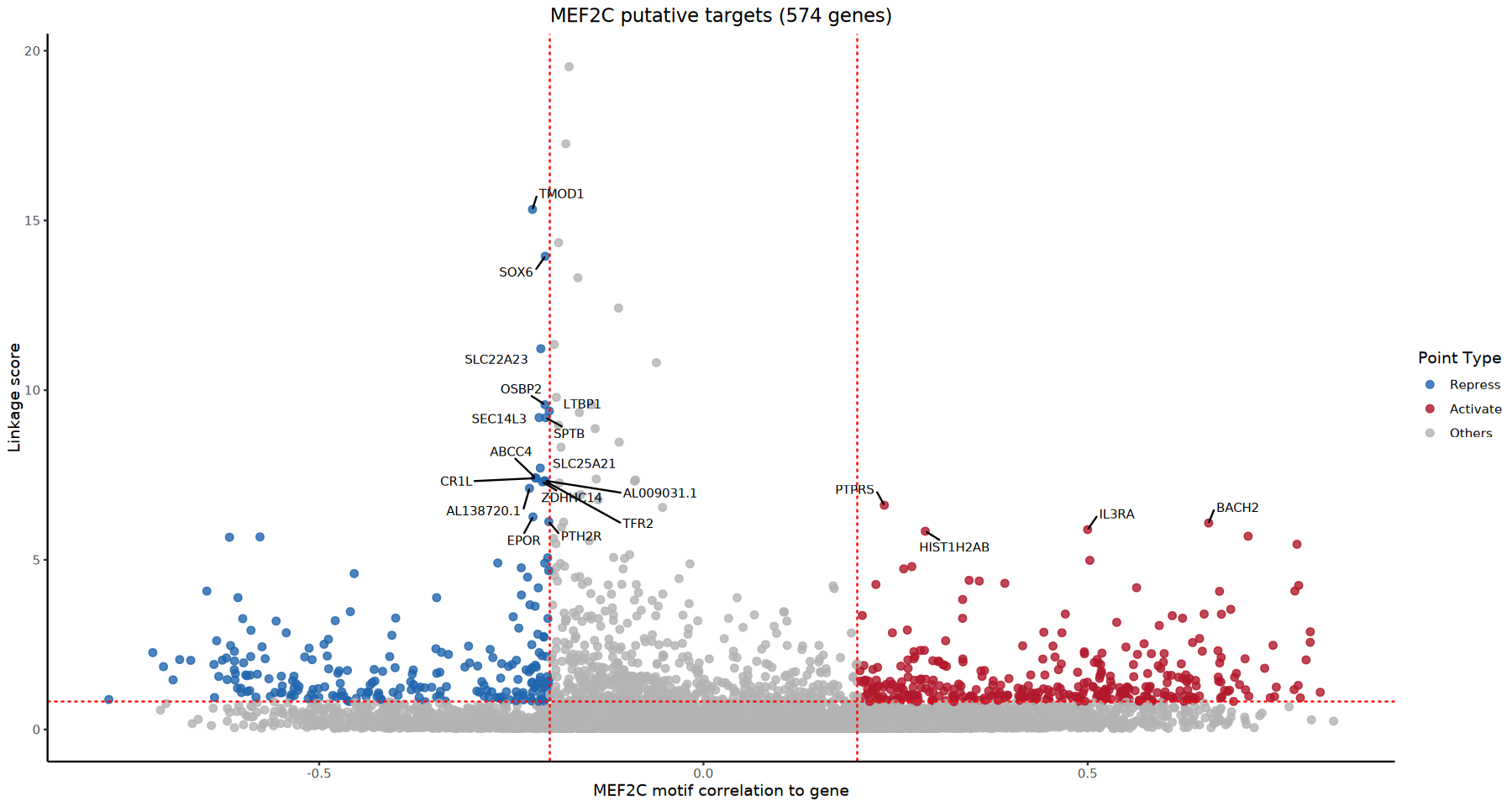

💡 说明：这里示例展示了其中一个TF下游调控的 Target 基因，完整图片去./result目录下找
Activate（激活型靶点，红色）：位于右上角（强正相关 + 高 Linkage），说明该 TF 极有可能直接结合并促进了该基因的表达。
Repress（抑制型靶点，蓝色）：位于左上角（强负相关 + 高 Linkage），说明该 TF 极有可能直接结合并抑制了该基因的表达。
我们使用 ggrepel 自动对得分最高的 Top 20 靶基因进行了文字标注，方便您快速锁定关键基因。

6.2 Trios 调控共变性热图 (Heatmap)

为了全局性地展示 TF、Peak 和 Target Gene 在不同细胞状态下的动态协同变化，我们将利用 ComplexHeatmap 绘制三联并排热图。

在单细胞多组学数据中，真实的调控信号往往被稀疏性（Drop-out）和背景噪音所掩盖。因此，在提取特征进行可视化前，代码对候选的 Trios 进行了严苛的多维生物学过滤与精细的数据转换，以确保呈现的是最具生物学代表性的核心调控网络：

核心过滤与处理逻辑：

核心靶基因网络提取（去除弱调控边）：一个 TF 可能在基因组上有成千上万个潜在结合位点，但并非所有结合都能产生实质性的转录输出。代码按 linkage_score 降序，强制每个 TF 仅保留 top_n_trios (如 Top 100) 个调控证据最强的靶基因，从而剥离边缘性的弱调控噪音，聚焦于该 TF 的核心靶标群。
细胞亚群特异性 TF 筛选（剥离管家型 TF）：决定细胞命运和状态的往往是具有高度组织或阶段特异性的转录因子。利用 FindAllMarkers 在各个细胞类型中进行差异表达分析，仅保留在特定细胞群中具有最高特异性表达的代表性转录因子。这有效地剔除了广泛表达但缺乏亚群特异性调控功能的“管家型（House-keeping）TF”，揭示了维持特定细胞状态的关键调控枢纽。
跨模态特征对齐（控制缺失值误差）：将提取出来的 TF、Peak 和 Target Gene 投射到拟 Bulk 矩阵中进行多组学对齐，强制剔除因测序深度或 Drop-out 导致在任一模态中均值为 0 的配对，避免由缺失值引起的假阳性共变信号。
动态高相关性双重检验（聚焦强驱动效应）：为了捕获最确凿的物理调控驱动效应，代码初始强制要求 TF-Gene表达相关性 和 TF表达-活性相关性 必须同时 > 0.5。若当前样本集数据质量或生物学异质性无法满足此严苛条件，内置算法将阶梯式降低阈值（0.4 -> 0.3 -> 0.2），在保证统计学下限的前提下，最大程度保留高度共变的精英三元组。
Pseudobulk 平滑化与 Z-score 标准化：在每种细胞类型内部构建 Pseudobulk 样本以填补单细胞极度的稀疏性空白；随后分别对三个维度的矩阵按行进行 Z-score 标准化（Scale）。这不仅消除了不同基因、不同 Peak 之间的本底表达/开放度差异，更将绝对数值尺度截然不同的 RNA 和 ATAC 数据统一到相同的统计学尺度，使得其相对变化趋势具有直接可比性。

trios_df_heatmap <- trios_df_filter

pdf_w <- 20 
pdf_h <- 10 
panel_cm <- 9 

if (nrow(trios_df) == 0) { 
  cat("警告: 过滤后没有剩余的 Trios，跳过热图绘制。\n") 
} else { 
  #cat("正在过滤 Trios 用于绘图...\n") 
  # 按 TF 分组，保留 Linkage Score Top N 的 Trios 
  heatmap_tmp <- trios_df_heatmap 
  trios_plot <- heatmap_tmp %>% 
    group_by(TF) %>% 
    arrange(desc(linkage_score)) %>% 
    slice_head(n = top_n_trios) %>% 
    ungroup() 

  # ========================================================================= 
  # 新的 TF 筛选逻辑: 基于细胞类型特异性 (FindAllMarkers) 选择 Top TF 
  # ========================================================================= 
  unique_all_tfs <- unique(trios_plot$TF) 
  
  # 确保 Idents 为用户指定的细胞类型分组列 
  meta <- data@meta.data 
  if (is.null(heatmap_group_by) || !heatmap_group_by %in% colnames(meta)) { 
    candidates <- c("celltype", "seurat_clusters", "Cluster", "CellType", "Annotation", "cell_type") 
    found <- intersect(candidates, colnames(meta)) 
    if (length(found) > 0) { 
      heatmap_group_by <- found[1] 
    } 
  } 
  Idents(data) <- heatmap_group_by 
  
  # 对选定的 TF 进行 FindAllMarkers 差异分析 
  # 【修复】：使用 suppressWarnings 屏蔽 Seurat V5 内部弃用警告
  tf_markers_all <- suppressWarnings(FindAllMarkers( 
    data, 
    assay = "RNA", 
    features = unique_all_tfs, 
    only.pos = TRUE, 
    min.pct = 0.01, 
    logfc.threshold = 0.1, 
    verbose = FALSE 
  ))
  
  if (nrow(tf_markers_all) > 0) { 
    # 选取各个 Idents (cluster) 中 avg_log2FC 最高的 1 个 TF 作为代表 
    top_tfs_per_cluster <- tf_markers_all %>% 
      group_by(cluster) %>% 
      slice_max(order_by = avg_log2FC, n = 1, with_ties = FALSE) %>% 
      ungroup() 
    
    top_10_tfs <- unique(top_tfs_per_cluster$gene) 
  } else { 
    # 如果没有找到显著的 marker，回退到按总分排序选 top 15 
    if ("linkage_score" %in% colnames(trios_plot)) { 
      tf_priority <- trios_plot %>% 
        group_by(TF) %>% 
        summarize(score_metric = sum(linkage_score, na.rm = TRUE)) %>% 
        arrange(desc(score_metric)) 
      top_10_tfs <- head(tf_priority$TF, 15) 
    } 
  } 

  trios_plot <- trios_plot %>% filter(TF %in% top_10_tfs) 

  # 8.2 准备 Pseudobulk 矩阵 (按 CellType 内部切分) 
  cell_groups <- split(rownames(meta), meta[[heatmap_group_by]]) 
  
  pb_list <- list()        # 存储每个 PB 包含的细胞 ID 
  pb_names <- c()          # 存储 PB 的唯一名称 (e.g., B_Cell_1) 
  pb_celltypes <- c()      # 存储 PB 所属的 CellType (e.g., B_Cell) 
  
  for (ct in names(cell_groups)) { 
    cells <- cell_groups[[ct]] 
    n_cells <- length(cells) 
    
    # 如果细胞数太少，至少保留一个 PB 
    if (n_cells < heatmap_pseudobulk_size ) { 
      pb_list[[paste0(ct, "_1")]] <- cells 
      pb_names <- c(pb_names, paste0(ct, "_1")) 
      pb_celltypes <- c(pb_celltypes, ct) 
    } else { 
      n_pbs <- ceiling(n_cells / heatmap_pseudobulk_size ) 
      #确保 n_pbs 至少为 1
      if (n_pbs < 1) n_pbs <- 1

      # 创建分组索引：如果只分1组，直接全给1，否则用 cut
      if (n_pbs == 1) {
        split_idx <- rep(1, length(cells))
      } else {
        split_idx <- as.numeric(cut(seq_along(cells), breaks = n_pbs))
      }
      chunked_cells <- split(cells, split_idx)
      
      for (i in names(chunked_cells)) { 
        pb_id <- paste0(ct, "_", i) 
        pb_list[[pb_id]] <- chunked_cells[[i]] 
        pb_names <- c(pb_names, pb_id) 
        pb_celltypes <- c(pb_celltypes, ct) 
      } 
    } 
  } 
  
  calc_mean_expr_list <- function(mat, groups_list) { 
    res <- matrix(NA, nrow = nrow(mat), ncol = length(groups_list)) 
    colnames(res) <- names(groups_list) 
    rownames(res) <- rownames(mat) 
    
    for (i in seq_along(groups_list)) { 
      cells <- groups_list[[i]] 
      valid_cells <- intersect(cells, colnames(mat)) 
      
      if (length(valid_cells) > 1) { 
        res[, i] <- rowMeans(mat[, valid_cells, drop = FALSE]) 
      } else if (length(valid_cells) == 1) { 
        res[, i] <- mat[, valid_cells] 
      } else { 
        res[, i] <- 0 
      } 
    } 
    return(res) 
  } 
  
  valid_tfs <- intersect(unique(trios_plot$TF), rownames(rna_data)) 
  mat_tf <- calc_mean_expr_list(rna_data[valid_tfs, , drop=FALSE], pb_list) 
  mat_tf <- t(scale(t(mat_tf))) 
  mat_tf[is.na(mat_tf)] <- 0 
  
  # 2. Peak Accessibility Matrix 
  # 【修复】：使用 suppressWarnings 屏蔽 GetAssayData 的 slot 弃用警告
  atac_data <- tryCatch({ 
    suppressWarnings(GetAssayData(data, assay = "ATAC", layer = "data"))
  }, error = function(e) { 
    suppressWarnings(GetAssayData(data, assay = "ATAC", slot = "data"))
  }) 
  
  valid_peaks <- intersect(unique(trios_plot$peak), rownames(atac_data)) 
  mat_peak <- calc_mean_expr_list(atac_data[valid_peaks, , drop=FALSE], pb_list) 
  mat_peak <- t(scale(t(mat_peak))) 
  mat_peak[is.na(mat_peak)] <- 0 
  
  # 3. Target Gene Expression Matrix 
  valid_genes <- intersect(unique(trios_plot$gene), rownames(rna_data)) 
  mat_gene <- calc_mean_expr_list(rna_data[valid_genes, , drop=FALSE], pb_list) 
  mat_gene <- t(scale(t(mat_gene))) 
  mat_gene[is.na(mat_gene)] <- 0 
  
  trios_plot_final_raw <- trios_plot %>% 
    filter(TF %in% rownames(mat_tf) & 
           peak %in% rownames(mat_peak) & 
           gene %in% rownames(mat_gene)) 
  
  if (nrow(trios_plot_final_raw) > 0) { 
    unique_tfs <- unique(trios_plot_final_raw$TF) 
    
    if (exists("tf_markers_all") && nrow(tf_markers_all) > 0) { 
      tf_celltype_mapping <- tf_markers_all %>% 
        dplyr::filter(gene %in% unique_tfs) %>% 
        dplyr::group_by(gene) %>% 
        dplyr::slice_max(order_by = avg_log2FC, n = 1, with_ties = FALSE) %>% 
        dplyr::ungroup() %>% 
        dplyr::select(TF = gene, celltype = cluster) 
    } else { 
      tf_celltype_mapping <- data.frame(TF = character(), celltype = character()) 
    } 
    
    missing_tfs <- setdiff(unique_tfs, tf_celltype_mapping$TF) 
    if (length(missing_tfs) > 0) { 
      tf_celltype_mapping <- bind_rows( 
        tf_celltype_mapping, 
        data.frame(TF = missing_tfs, celltype = "Unknown") 
      ) 
    } 
    
    col_celltype_order <- unique(pb_celltypes) 
    
    ordered_tfs <- c() 
    for (ct in col_celltype_order) { 
      tfs_in_ct <- tf_celltype_mapping$TF[tf_celltype_mapping$celltype == ct] 
      tfs_in_ct_ordered <- intersect(top_10_tfs, tfs_in_ct) 
      ordered_tfs <- c(ordered_tfs, tfs_in_ct_ordered) 
    } 
    tfs_unknown <- tf_celltype_mapping$TF[tf_celltype_mapping$celltype == "Unknown"] 
    ordered_tfs <- c(ordered_tfs, intersect(top_10_tfs, tfs_unknown)) 
    
    trios_plot_final_raw <- trios_plot_final_raw %>% 
      mutate(TF = factor(TF, levels = ordered_tfs)) %>% 
      arrange(TF, desc(if("linkage_score" %in% names(.)) linkage_score else abs(peak_gene_cor))) 
      
    # ========================================================================= 
    # 【新增功能】：动态降级相关性阈值
    # ========================================================================= 
    thresholds_to_try <- c(0.5, 0.4, 0.3, 0.2)
    trios_plot_final <- NULL
    applied_threshold <- NA
    
    for (thresh in thresholds_to_try) {
      temp_filtered <- trios_plot_final_raw[which(trios_plot_final_raw$tf_gene_cor > thresh & trios_plot_final_raw$tf_activity_cor > thresh),]
      if (nrow(temp_filtered) > 0) {
        trios_plot_final <- temp_filtered
        applied_threshold <- thresh
        if (thresh < 0.5) {
          cat(sprintf("提示: 阈值 0.5 时数据为空，已自动将相关性阈值降至 %.1f 进行绘图。\n", thresh))
        }
        break # 找到数据就跳出循环
      }
    }
    
    # 检查经过降级尝试后，是否最终还是没数据
    if (is.null(trios_plot_final) || nrow(trios_plot_final) == 0) {
      cat("警告: 即使将相关性阈值降至最低 (0.2)，依然没有剩余的 Trios，跳过热图绘制。\n")
    } else {
      trios_plot_final$TF <- droplevels(trios_plot_final$TF) 
      
      plot_mat_tf <- mat_tf[as.character(trios_plot_final$TF), , drop=FALSE] 
      plot_mat_peak <- mat_peak[as.character(trios_plot_final$peak), , drop=FALSE] 
      plot_mat_gene <- mat_gene[as.character(trios_plot_final$gene), , drop=FALSE] 
      
      rownames(plot_mat_tf) <- NULL 
      rownames(plot_mat_peak) <- NULL 
      rownames(plot_mat_gene) <- NULL 
      
      col_peak <- colorRamp2(c(-1.5, 0, 1.5), c("#2166ac", "white", "#b2182b")) 
      col_tf <- colorRamp2(c(-2, 0, 2), c("#762a83", "white", "#1b7837")) 
      col_gene <- colorRamp2(c(-2, 0, 2), c("#4d4d4d", "white", "#d73027")) 
      
      unique_groups <- unique(pb_celltypes) 
      n_groups <- length(unique_groups) 
      if (n_groups <= 8) { 
        grp_cols <- brewer.pal(max(3, n_groups), "Set2")[1:n_groups] 
      } else { 
        grp_cols <- colorRampPalette(brewer.pal(8, "Set2"))(n_groups) 
      } 
      names(grp_cols) <- unique_groups 
      ha_top <- HeatmapAnnotation( 
        Celltype = pb_celltypes, 
        col = list(Celltype = grp_cols), 
        show_legend = TRUE, 
        show_annotation_name = TRUE 
      ) 
      
      unique_tfs_levels <- levels(trios_plot_final$TF) 
      tf_colors <- colorRampPalette(brewer.pal(8, "Set1"))(length(unique_tfs_levels)) 
      names(tf_colors) <- unique_tfs_levels 
      
      ha_left <- rowAnnotation( 
        TF = trios_plot_final$TF, 
        col = list(TF = tf_colors), 
        show_annotation_name = TRUE, 
        annotation_name_side = "top", 
        show_legend = TRUE 
      ) 
      
      mark_at <- numeric(0) 
      mark_labels <- character(0) 
      
      unique_tfs_plot <- unique(trios_plot_final$TF) 
      for (tf in unique_tfs_plot) { 
        tf_indices <- which(trios_plot_final$TF == tf) 
        genes_in_tf <- trios_plot_final$gene[tf_indices] 
        top_unique_genes <- unique(genes_in_tf)[1:min(5, length(unique(genes_in_tf)))] 
        
        for (g in top_unique_genes) { 
          first_match_idx <- tf_indices[match(g, genes_in_tf)] 
          mark_at <- c(mark_at, first_match_idx) 
          mark_labels <- c(mark_labels, g) 
        } 
      } 
      
      if (length(mark_at) > 0) {
        ha_right <- rowAnnotation( 
          link = anno_mark( 
            at = mark_at, 
            labels = mark_labels, 
            labels_gp = gpar(fontsize = 8), 
            link_width = unit(4, "mm"), 
            padding = unit(1, "mm") 
          ) 
        ) 
      }
      
      ht1 <- Heatmap( 
        plot_mat_tf, 
        name = "TF Expr", 
        col = col_tf, 
        cluster_rows = FALSE, 
        cluster_columns = FALSE, 
        show_row_names = TRUE, 
        show_column_names = FALSE, 
        top_annotation = ha_top, 
        left_annotation = ha_left, 
        column_title = "TF Expression", 
        width = unit(panel_cm, "cm"), 
        row_order = seq_len(nrow(plot_mat_tf)), 
        row_title_rot = 0, 
        row_title_gp = gpar(fontsize = 10, fontface = "bold"), 
        use_raster = TRUE 
      ) 
      
      ht2 <- Heatmap( 
        plot_mat_peak, 
        name = "Peak Access", 
        col = col_peak, 
        cluster_rows = FALSE, 
        cluster_columns = FALSE, 
        show_row_names = FALSE, 
        show_column_names = FALSE, 
        top_annotation = ha_top, 
        column_title = "Peak Accessibility", 
        width = unit(panel_cm, "cm"), 
        use_raster = TRUE 
      ) 
      
      ht3 <- Heatmap( 
        plot_mat_gene, 
        name = "Gene Expr", 
        col = col_gene, 
        cluster_rows = FALSE, 
        cluster_columns = FALSE, 
        show_row_names = FALSE, 
        show_column_names = FALSE, 
        top_annotation = ha_top, 
        column_title = "Target Gene Expr", 
        width = unit(panel_cm, "cm"), 
        use_raster = TRUE 
      ) 
      
      # 【修复】：根据是否有标签组装热图
      if (length(mark_at) > 0) {
        ht_list <- ht1 + ht2 + ht3 + ha_right 
      } else {
        ht_list <- ht1 + ht2 + ht3
      }
      
      # 在输出文件名中带上最终使用的阈值，方便你区分
      out_prefix <- sprintf("/complex_heatmap_annotated_cor_%.1f", applied_threshold)
      
      pdf(paste0(output_path, out_prefix, ".pdf"), width = pdf_w, height = pdf_h) 
      draw(ht_list, main_heatmap = "TF Expr", merge_legend = TRUE) 
      dev.off() 
      
      png(paste0(output_path, out_prefix, ".png"),  width = pdf_w, height = pdf_h, units = "in", res = 300) 
      draw(ht_list, main_heatmap = "TF Expr", merge_legend = TRUE) 
      dev.off() 
      
      saveRDS(ht_list, paste0(output_path, out_prefix, ".rds")) 
    }
  } else { 
    #cat("警告: 最终绘图矩阵为空。\n") 
  } 
}

ht_list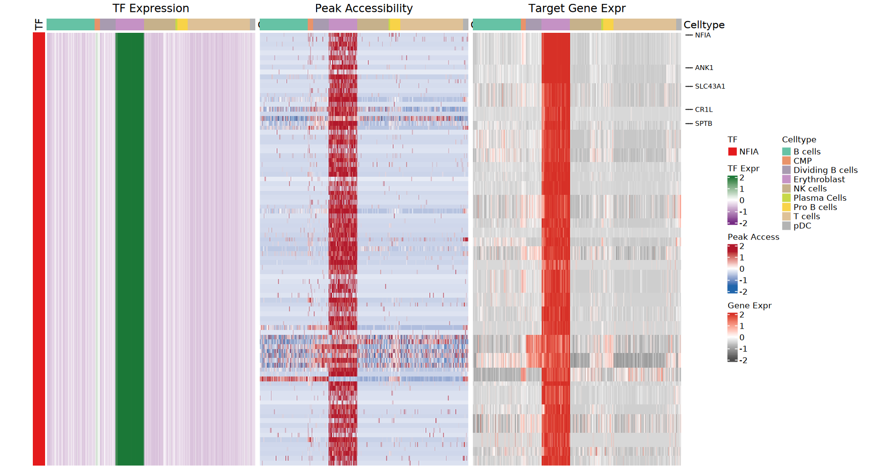

💡 说明：
在最终生成的热图中，请横向追踪信号的传递。对于一个真实且活跃的正向调控三元组，您将观察到显著的“跨模态共变”：在特定细胞群中，TF 的表达上调（左图高信号），驱动了其对应结合 Peak 染色质可及性的增加（中图高信号），最终导致下游核心靶基因群的转录激活（右图高信号）。

6.3 核心 TF 靶基因群的亚群特异性表达热图

在全局性的多组学共变热图（5.3 节）中，我们验证了 TF、Peak 与 Target 之间的顺式调控关系。接下来，我们需要进一步验证这些由核心 TF 驱动的靶基因网络（Target Gene Modules），是否真正决定了细胞的异质性与分型。

本部分代码将逐一提取前述分析中锁定的 Top 10 核心转录因子，并专门绘制其专属靶基因群在各个细胞亚群中的表达热图（Expression Heatmap）。

数据处理与可视化逻辑：

靶基因截取与矩阵投射：对于每个目标 TF，依据 linkage_score 提取其强效驱动的 Top 靶基因群（由 top_n_genes_per_tf_heatmap 参数控制）。随后，从单细胞转录组矩阵中精确提取这些靶基因在所有有效细胞中的表达谱。
基于亚群的矩阵聚合（矩阵乘法）：为了消除单细胞层面的稀疏噪音并突出细胞群间的宏观差异，代码通过构建模型矩阵（model.matrix），利用高效的矩阵乘法计算出各个靶基因在每个细胞亚群中的平均表达量。
特征标准化与双向聚类：对聚合后的均值矩阵按行执行 Z-score 标准化。在绘图时，同时启用行（基因）和列（细胞群）的无监督层次聚类（Hierarchical Clustering）。

# ==============================================================================
# 1. 定义绘图函数 (增加了 return(ht))
# ==============================================================================
plot_tf_targets_heatmap <- function(tf_name, trios_df, seurat_obj, celltype_col = "shoudong", output_dir = NULL, top_n_genes = top_n_genes_per_tf_heatmap) { 
  #cat(sprintf("正在为 TF: %s 绘制靶基因表达热图...\n", tf_name)) 
  
  targets <- trios_df %>% 
    filter(TF == tf_name) %>% 
    dplyr::select(gene, linkage_score) %>% 
    distinct() %>% 
    arrange(desc(linkage_score)) 
  
  if (nrow(targets) == 0) { 
    #cat(sprintf("警告: 未找到 TF %s 的靶基因，跳过绘图。\n", tf_name)) 
    return(NULL) 
  } 
  
  if (nrow(targets) > top_n_genes) { 
    #cat(sprintf("靶基因数量 (%d) 较多，仅展示 Linkage Score 最高的 %d 个。\n", nrow(targets), top_n_genes)) 
    plot_genes <- targets$gene[1:top_n_genes] 
  } else { 
    plot_genes <- targets$gene 
  } 
  
  if (!celltype_col %in% colnames(seurat_obj@meta.data)) { 
    #cat(sprintf("警告: Seurat 对象中未找到 '%s' 列，尝试使用 'seurat_clusters' 或 'Ident'。\n", celltype_col)) 
    if ("seurat_clusters" %in% colnames(seurat_obj@meta.data)) { 
      celltype_col <- "seurat_clusters" 
    } else { 
      celltype_col <- "ident" 
    } 
    #cat(sprintf("已切换为使用 '%s' 进行分组。\n", celltype_col)) 
  } 
  
  expr_data <- tryCatch({ 
    GetAssayData(seurat_obj, assay = "RNA", layer = "data") 
  }, error = function(e) { 
    GetAssayData(seurat_obj, assay = "RNA", slot = "data") 
  }) 
  
  valid_genes <- intersect(plot_genes, rownames(expr_data)) 
  if (length(valid_genes) < 2) { 
    #cat("警告: 有效基因数量不足 (<2)，无法绘制热图。\n") 
    return(NULL) 
  } 
  
  idents <- seurat_obj@meta.data[[celltype_col]] 
  if (is.null(idents)) idents <- Idents(seurat_obj) 
  
  valid_cells <- !is.na(idents) 
  expr_subset <- expr_data[valid_genes, valid_cells, drop=FALSE] 
  idents_subset <- idents[valid_cells] 
  
  mm <- model.matrix(~ 0 + factor(idents_subset)) 
  colnames(mm) <- levels(factor(idents_subset)) 
  mat_sum <- expr_subset %*% mm 
  mat_count <- colSums(mm) 
  mat_avg <- t(t(mat_sum) / mat_count) 
  
  mat_scale <- t(scale(t(mat_avg))) 
  col_fun <- colorRamp2(c(-2, 0, 2), c("#440154FF", "#21908CFF", "#FDE725FF")) 
  
  celltypes <- colnames(mat_scale) 
  ct_colors <- suppressWarnings(colorRampPalette(RColorBrewer::brewer.pal(8, "Set2"))(length(celltypes)))
  names(ct_colors) <- celltypes 
  
  ha_bottom <- HeatmapAnnotation( 
    Celltype = celltypes, 
    col = list(Celltype = ct_colors), 
    show_legend = TRUE, 
    show_annotation_name = TRUE 
  ) 
  
  ht <- Heatmap(mat_scale, 
                name = "Z-score", 
               # col = col_fun, 
                col = col_peak, 
                cluster_rows = TRUE, 
                show_row_names = FALSE, 
                row_title = paste0("Target Genes (n=", length(valid_genes), ")"), 
                cluster_columns = TRUE, 
                show_column_names = TRUE, 
                column_names_rot = 90,
                show_column_dend = FALSE,
                show_row_dend = FALSE,
                column_title = paste0("Expression in ", tf_name, " Trios"), 
                bottom_annotation = ha_bottom, 
                use_raster = TRUE 
  ) 
  
  if (!is.null(output_dir)) { 
    dir.create(output_dir, recursive = TRUE, showWarnings = FALSE) 
    filename <- file.path(output_dir, paste0(tf_name, "_targets_heatmap.pdf")) 
    pdf(filename, width = 8, height = 4) 
    draw(ht) 
    dev.off() 
    #cat(sprintf("靶基因热图已保存至: %s\n", filename)) 
  } 
  
  return(ht) # 【新增】必须返回对象供后续转换为Base64
}

dir.create(heatmap_out_dir, recursive = TRUE, showWarnings = FALSE)

# 辅助函数：保存 ComplexHeatmap 为 PNG 并转为 Base64
save_and_encode_heatmap <- function(ht, filename_base, width = 8, height = 4) {
  full_path_pdf <- paste0(filename_base, ".pdf")
  temp_png <- tempfile(fileext = ".png")
  
  # 保存 PDF (高分辨率，供点击下载)
  pdf(full_path_pdf, width = width, height = height)
  draw(ht)
  invisible(dev.off())
  
  # 保存临时 PNG (用于网页内嵌展示)
  png(temp_png, width = width * 100, height = height * 100, res = 100)
  draw(ht)
  invisible(dev.off())
  return(NULL)
}

plot_list <- list()
for (tf in top_10_tfs) { 
  # 调用绘图函数 (设为 NULL 避免函数内重复保存，由外部统一保存)
  ht <- tryCatch({ 
    plot_tf_targets_heatmap(tf, trios_df, seurat_obj = data, celltype_col = celltype_col, output_dir = NULL, top_n_genes = top_n_genes_per_tf_heatmap) 
  }, error = function(e) { 
    #cat(sprintf("绘制 TF %s 热图失败: %s\n", tf, e$message)) 
    return(NULL)
  }) 
  
  if (!is.null(ht)) {
    file_base <- file.path(heatmap_out_dir, paste0(tf, "_targets_heatmap"))
    res <- save_and_encode_heatmap(ht, file_base)
  }
}

ht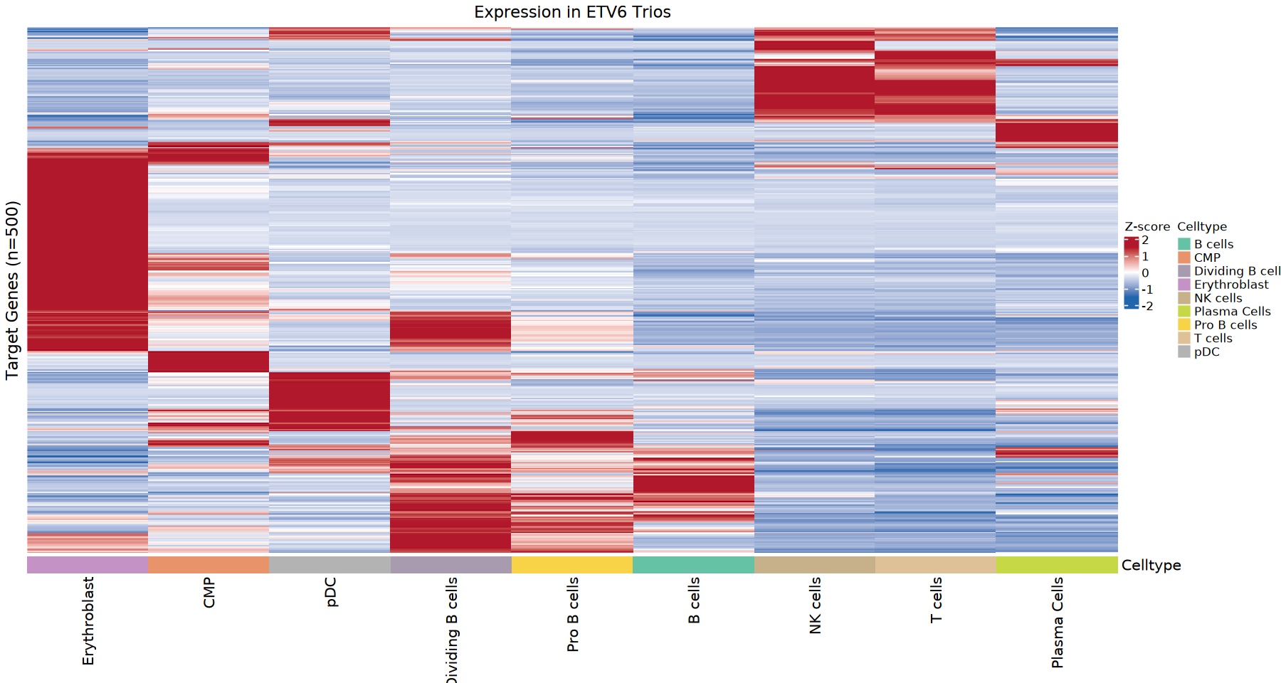

💡 说明：示例展示了其中一个TF调控的 Target 基因在不同细胞类型中的表达情况，完整结果去.result目录下找
列聚类验证：观察热图顶部的细胞群分支树。如果该 TF 是某个细胞谱系的主效调节因子（Master Regulator），您将看到其靶基因群的表达模式能完美地将该靶细胞群与其他细胞群区分开来（形成独立分支）。
基因共表达模块：纵向观察，颜色深红（高 Z-score）的区块代表了该 TF 在特定细胞状态下集中激活的下游基因网络，这为后续精细刻画细胞状态的分子特征提供了直接的靶点列表。

6.4 TF-Target 调控网络图

为了直观解析转录因子的辐射状调控拓扑结构，本部分代码利用 igraph 构建并绘制了以核心 TF 为中心的星型调控网络图（Regulatory Network）。

生物学逻辑与网络映射规则：

节点（Nodes）过滤与映射：
- 节点筛选：并非所有高分靶基因都会被绘制。代码计算了所有靶基因在整体细胞中的平均表达水平（AverageExpression），并剔除极低表达的背景基因（依据 min_expr_percentile 参数）。这保证了网络中的靶标不仅有调控潜力，而且在当前组织中具有真实的转录活性。
- 节点大小（Size）：节点的物理面积严格映射自基因的对数化平均表达量（log1p(expression)）。节点越大，表明该基因在细胞体系中的本底转录活性越高。
- 节点颜色（Color）：中心转录因子（TF）被固定标记为醒目的橙色（Hub 节点），以凸显其网络枢纽地位。
边（Edges）的物理与统计学映射：
- 边粗细（Width）：连线的粗细直接映射自该调控对的 Linkage Score。线条越粗，代表多组学证据（TF 结合亲和力与 Peak 可及性）支持该调控轴的物理强度越高。
- 边颜色（Edge Color）：严格反映调控的方向性。红色（红线）代表正相关，指示该 TF 对靶标的转录激活（Activation）；蓝色（蓝线）代表负相关，指示转录抑制（Repression）。
拓扑布局：采用 Fruchterman-Reingold (FR) 力导向布局算法（layout_with_fr）。该算法会根据调控边权重自动调整节点距离，使得与中心 TF 关联最紧密、调控最强的核心靶基因被物理“拉”向网络中心，从而清晰呈现核心到边缘的层级调控结构。

options(warn = -1)  # 关闭警告
# ==============================================================================
# 1. 定义网络图绘制函数 (增加了返回值 g 和 layout)
# ============================================================================== 
plot_tf_network <- function(tf_name, trios_df, seurat_obj, output_dir = NULL, 
                            min_expr_percentile = 0.2, 
                            max_nodes = 50) {          
  #cat(sprintf("正在为 TF: %s 绘制调控网络图...\n", tf_name)) 
  
  # 1. 筛选 Target 数据
  target_data <- trios_df %>% 
    filter(TF == tf_name) %>% 
    mutate(correlation = if("tf_gene_cor" %in% names(.)) tf_gene_cor else peak_gene_cor) %>% 
    group_by(gene) %>% 
    summarize( 
      linkage_score = max(linkage_score, na.rm = TRUE), 
      correlation = mean(correlation, na.rm = TRUE),    
      .groups = "drop" 
    ) %>% 
    arrange(desc(linkage_score)) 
  
  if (nrow(target_data) == 0) return(NULL) 
  
  # 2. 获取表达量
  all_genes <- rownames(GetAssayData(seurat_obj, assay = "RNA")) 
  valid_features <- intersect(c(tf_name, target_data$gene), all_genes) 
  
  if (length(valid_features) == 0) return(NULL) 
  
  avg_expr_list <- AverageExpression(seurat_obj, features = valid_features, assay = "RNA") 
  if ("RNA" %in% names(avg_expr_list)) { 
    avg_expr <- avg_expr_list$RNA 
  } else { 
    avg_expr <- avg_expr_list[[1]] 
  } 
  
  if (is.null(avg_expr) || nrow(avg_expr) == 0) { 
     gene_expr_vals <- setNames(rep(0, length(valid_features)), valid_features) 
  } else { 
     gene_expr_vals <- rowMeans(avg_expr) 
  } 
  
  get_expr <- function(genes, expr_vec) { 
    vals <- expr_vec[genes] 
    vals[is.na(vals)] <- 0 
    return(vals) 
  } 
  target_data$expression <- get_expr(target_data$gene, gene_expr_vals) 
  
  # 3. 过滤
  if (max(target_data$expression) > 0) { 
      expr_threshold <- quantile(target_data$expression[target_data$expression > 0], min_expr_percentile, na.rm = TRUE) 
      target_data_filtered <- target_data %>% filter(expression >= expr_threshold) 
  } else { 
      target_data_filtered <- target_data 
  } 
  
  if (nrow(target_data_filtered) > max_nodes) { 
    target_data_filtered <- head(target_data_filtered, max_nodes) 
  } 
  
  if (nrow(target_data_filtered) == 0) return(NULL) 
  
  # 4. 构建网络
  tf_expr_val <- get_expr(tf_name, gene_expr_vals) 
  if (tf_expr_val == 0 && nrow(target_data_filtered) > 0) tf_expr_val <- max(target_data_filtered$expression) 
   
  # 准备节点属性
  target_cors <- target_data_filtered$correlation 
  target_cors[is.na(target_cors)] <- 0 
  
  nodes_df <- data.frame( 
    id = c(tf_name, target_data_filtered$gene), 
    type = c("TF", rep("Target", nrow(target_data_filtered))), 
    expression = c(tf_expr_val, target_data_filtered$expression), 
    correlation = c(0, target_cors), 
    stringsAsFactors = FALSE 
  ) 
  
  # 准备边属性
   edge_colors <- ifelse(target_data_filtered$correlation > 0, "#b2182b", "#2166ac") 
   edges_df <- data.frame( 
     from = tf_name, 
     to = target_data_filtered$gene, 
     weight = target_data_filtered$linkage_score, 
     color = edge_colors 
   ) 
   
   g <- graph_from_data_frame(d = edges_df, vertices = nodes_df, directed = TRUE) 
   
   # 5. 设置绘图样式 
   expr_scaled <- log1p(V(g)$expression) 
  
  # 节点大小：基于表达量
  if (max(expr_scaled) == min(expr_scaled)) { 
      size_vec <- rep(10, length(expr_scaled)) 
  } else { 
      size_vec <- scales::rescale(expr_scaled, to = c(5, 15)) 
  } 
  # TF 节点稍微大一点
  V(g)$size <- size_vec 
  V(g)$size[V(g)$type == "TF"] <- 25 
  
  color_vec <- rep("#2166ac", vcount(g)) # 默认蓝色 (负相关) 
  color_vec[V(g)$correlation > 0] <- "#b2182b" # 正相关红色 
  color_vec[V(g)$type == "TF"] <- "#FDB462" # TF 橙色 (保持不变)
  V(g)$color <- adjustcolor(color_vec, alpha.f = 0.8) 
  
  # 边宽度：基于 Linkage Score
  if (max(E(g)$weight) == min(E(g)$weight)) { 
      E(g)$width <- 1.5 
  } else { 
      E(g)$width <- scales::rescale(E(g)$weight, to = c(0.5, 3)) 
  } 
  E(g)$arrow.size <- 0.3
  E(g)$curved <- 0.2 # 稍微弯曲的边更美观
  
  # 标签样式
  V(g)$label <- V(g)$name 
  V(g)$label.color <- "black" 
  V(g)$label.cex <- ifelse(V(g)$type == "TF", 1.2, 0.7)
  V(g)$label.font <- 2 
  
  # 布局算法
  l <- layout_with_fr(g) 
  
  # 保存 PDF
  if (!is.null(output_dir)) { 
    dir.create(output_dir, recursive = TRUE, showWarnings = FALSE) 
    filename <- file.path(output_dir, paste0(tf_name, "_network.pdf")) 
    pdf(filename, width = 8, height = 8) 
    plot(g, layout = l, main = paste0(tf_name, " Network"), vertex.frame.color = "white", margin = c(0,0,0,0)) 
    legend("bottomright", legend = c("TF", "Pos Cor", "Neg Cor"), col = c("#FDB462", "#b2182b", "#2166ac"), pch = 19, pt.cex = 1.5, bty = "n") 
    dev.off() 
  } 
  
  return(list(g = g, layout = l))
}

dir.create(network_out_dir, recursive = TRUE, showWarnings = FALSE)

# 辅助函数：绘制 igraph 并保存为 Base64
save_and_encode_network <- function(g, layout, filename_base, width = 8, height = 8) {
  full_path_pdf <- paste0(filename_base, ".pdf")
  temp_png <- tempfile(fileext = ".png")
  
  # 保存 PDF
  pdf(full_path_pdf, width = width, height = height)
  plot(g, layout = layout, vertex.frame.color = "white", margin = c(0,0,0,0))
  legend("bottomright", legend = c("TF", "Pos Cor", "Neg Cor"), col = c("#FDB462", "#b2182b", "#2166ac"), pch = 19, pt.cex = 1.5, bty = "n")
  invisible(dev.off())
  
  # 保存 PNG 
  png(temp_png, width = width * 100, height = height * 100, res = 100)
  plot(g, layout = layout, vertex.frame.color = "white", margin = c(0,0,0,0))
  legend("bottomright", legend = c("TF", "Pos Cor", "Neg Cor"), col = c("#FDB462", "#b2182b", "#2166ac"), pch = 19, pt.cex = 1.5, bty = "n")
  invisible(dev.off())
  return(NULL)
}

plot_list <- list()

for (tf in top_10_tfs) {
  # 调用绘图函数
  res_obj <- tryCatch({
    plot_tf_network(tf, trios_df, seurat_obj = data, output_dir = NULL, max_nodes = network_max_nodes)
  }, error = function(e) return(NULL))
  
  if (!is.null(res_obj)) {
    file_base <- file.path(network_out_dir, paste0(tf, "_network"))
    res_img <- save_and_encode_network(res_obj$g, res_obj$layout, file_base)
  }
}
options(warn = 0)   # 恢复警告

 plot(res_obj$g, layout = res_obj$layout, vertex.frame.color = "white", margin = c(0,0,0,0))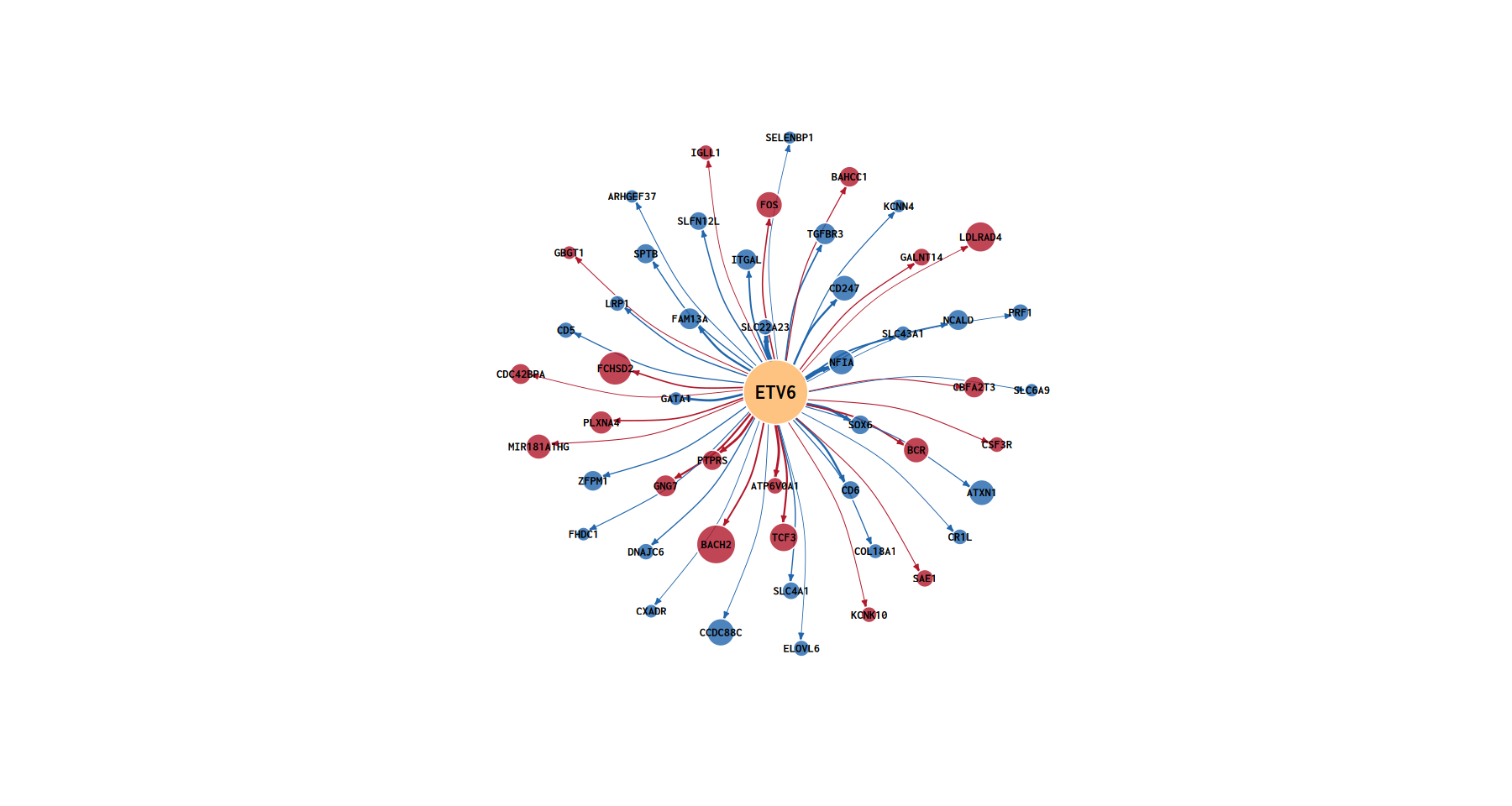

💡 说明：在观察生成的星型网络图时，请重点关注距离中心橙色 TF 最近，且节点面积最大的那些基因。它们不仅受该 TF 的强力物理驱动（连线最粗），而且自身转录极为活跃（节点最大），通常是介导该 TF 下游核心生物学功能的关键效应器（Key Effectors）。此外，通过红蓝连线的比例，可以快速评估该 TF 在当前细胞状态下是一个全局性的转录激活子（Activator）还是抑制子（Repressor）。

6.5 全局多转录因子协同调控网络图 (Global Regulatory Network)

在单 TF 视角的网络（6.4 节）中，我们只能看到“一对多”的星型结构。然而，在真实的生物学体系中，核心转录因子往往存在密集的协同调控（Co-regulation）与交叉互作（Cross-talk）。

本部分代码利用 igraph 并结合定制化的几何拓扑算法，构建了整合多个核心 TF 的全局调控网络。它不仅能揭示单个 TF 的势力范围，更能直观地暴露转录因子之间共享的靶基因模块（Shared Target Modules）。

核心拓扑算法与生物学映射规则：

核心枢纽提取与表达量映射：
- 基于总 Linkage Score，提取当前细胞体系中调控权重最高的 Top TFs（如 Top 20）。
- 节点的物理大小严密映射自其在 scRNA-seq 中的平均表达量（log1p(expression)）。
- 根据网络度（Degree，即连接的边数），动态调整核心 TF 的展示比例：出度越高的 TF 节点越大，直观凸显其在整个全局网络中的 Master Regulator（主调控因子）地位。
模块检测与 Louvain 聚类（Community Detection）：
- 代码在构建无向网络后，内部调用了 cluster_louvain 算法（基于模块度优化的社区发现算法）。
- 这一步在后台静默运行，它通过追踪边权重（Linkage Score），将整个庞大网络划分为多个紧密互作的亚模块（Modules），并将结果输出至 All_TFs_network_modules.txt 文件，为后续提取特定生物学通路基因集提供了数据基础。
定制化环形与放射状拓扑布局（Geometric Layout）：
- 核心 TF 环（TF Ring）：强制将所有 Hub TFs 均匀分布在一个内环上，确保核心枢纽不被海量靶基因淹没。
- 共享靶点（Shared Targets）：那些被两个或多个 TF 共同调控的靶基因（出度 > 1），其坐标通过向量均值（Vector Mean）被精确计算，并放置在对应 TF 之间的夹角内环。这些节点代表了关键的调控交叉点（Cross-talk Hubs）。
- 独占靶点（Unique Targets）：仅受单一 TF 调控的专属靶基因，则通过切线向量计算，呈放射状排布于该 TF 的外围（Outer Layer）。

plot_all_tf_network <- function(trios_df, seurat_obj, output_dir = NULL,
                                max_tfs = 20,
                                max_targets_per_tf = 50,
                                min_expr_percentile = 0.2,
                                detect_modules = TRUE,
                                tf_ring_expand = 1.35,
                                shared_target_inner_shrink = 0.72,
                                unique_target_outer_expand = 0.22,
                                shared_target_spread = 0.12,
                                max_target_labels = Inf) {
  edge_df <- trios_df %>%
    mutate(correlation = if ("tf_gene_cor" %in% names(.)) tf_gene_cor else peak_gene_cor) %>%
    group_by(TF, gene) %>%
    summarize(
      linkage_score = max(linkage_score, na.rm = TRUE),
      correlation = mean(correlation, na.rm = TRUE),
      .groups = "drop"
    )

  tf_rank <- edge_df %>%
    group_by(TF) %>%
    summarize(total_linkage = sum(linkage_score, na.rm = TRUE), .groups = "drop") %>%
    arrange(desc(total_linkage)) %>%
    head(max_tfs) %>%
    pull(TF)

  edge_df <- edge_df %>%
    filter(TF %in% tf_rank) %>%
    group_by(TF) %>%
    arrange(desc(linkage_score), .by_group = TRUE) %>%
    slice_head(n = max_targets_per_tf) %>%
    ungroup()

  if (nrow(edge_df) == 0) return(NULL)

  all_genes <- rownames(GetAssayData(seurat_obj, assay = "RNA"))
  features <- intersect(unique(c(edge_df$TF, edge_df$gene)), all_genes)
  if (length(features) == 0) return(NULL)

  avg_expr_list <- AverageExpression(seurat_obj, features = features, assay = "RNA")
  avg_expr <- if ("RNA" %in% names(avg_expr_list)) avg_expr_list$RNA else avg_expr_list[[1]]
  expr_vec <- if (is.null(avg_expr) || nrow(avg_expr) == 0) {
    setNames(rep(0, length(features)), features)
  } else {
    rowMeans(avg_expr)
  }

  edge_df$target_expr <- expr_vec[edge_df$gene]
  edge_df$target_expr[is.na(edge_df$target_expr)] <- 0

  if (max(edge_df$target_expr) > 0) {
    expr_cut <- quantile(edge_df$target_expr[edge_df$target_expr > 0], min_expr_percentile, na.rm = TRUE)
    edge_df <- edge_df %>% filter(target_expr >= expr_cut)
  }

  if (nrow(edge_df) == 0) return(NULL)

  target_stat <- edge_df %>%
    group_by(gene) %>%
    summarize(
      expression = max(target_expr, na.rm = TRUE),
      cor_mean = mean(correlation, na.rm = TRUE),
      .groups = "drop"
    )

  tf_stat <- edge_df %>%
    group_by(TF) %>%
    summarize(
      expression = ifelse(TF[1] %in% names(expr_vec), expr_vec[TF[1]], 0),
      degree_like = n(),
      .groups = "drop"
    )

  nodes_tf <- data.frame(
    name = tf_stat$TF,
    type = "TF",
    expression = tf_stat$expression,
    cor_mean = 0,
    degree_like = tf_stat$degree_like,
    stringsAsFactors = FALSE
  )

  nodes_target <- data.frame(
    name = target_stat$gene,
    type = "Target",
    expression = target_stat$expression,
    cor_mean = target_stat$cor_mean,
    degree_like = 0,
    stringsAsFactors = FALSE
  )

  nodes <- bind_rows(nodes_tf, nodes_target) %>%
    group_by(name) %>%
    summarize(
      type = ifelse(any(type == "TF"), "TF", "Target"),
      expression = max(expression, na.rm = TRUE),
      cor_mean = mean(cor_mean, na.rm = TRUE),
      degree_like = max(degree_like, na.rm = TRUE),
      .groups = "drop"
    )

  edge_colors <- ifelse(edge_df$correlation > 0, "#d73027", "#4575b4")
  edges <- data.frame(
    from = edge_df$TF,
    to = edge_df$gene,
    weight = edge_df$linkage_score,
    color = edge_colors,
    stringsAsFactors = FALSE
  )

  g <- igraph::graph_from_data_frame(edges, vertices = nodes, directed = TRUE)

  if (detect_modules && vcount(g) > 2 && ecount(g) > 0) {
    g_mod <- igraph::as.undirected(
      igraph::simplify(g, remove.multiple = TRUE, remove.loops = TRUE,
                       edge.attr.comb = list(weight = "sum", color = "first")),
      mode = "collapse",
      edge.attr.comb = list(weight = "sum", color = "first")
    )
    if (ecount(g_mod) > 0) {
      cl <- igraph::cluster_louvain(g_mod, weights = E(g_mod)$weight)
      mod_map <- igraph::membership(cl)
      V(g)$module_id <- as.integer(mod_map[V(g)$name])
    } else {
      V(g)$module_id <- rep(1L, vcount(g))
    }
  } else {
    V(g)$module_id <- rep(1L, vcount(g))
  }

  v_type <- V(g)$type
  v_expr <- V(g)$expression
  v_deg <- igraph::degree(g, mode = "all")

  tf_idx <- which(v_type == "TF")
  tg_idx <- which(v_type == "Target")

  size_vec <- rep(5, vcount(g))
  if (length(tf_idx) > 0) {
    tf_deg <- v_deg[tf_idx]
    size_vec[tf_idx] <- if (max(tf_deg) == min(tf_deg)) 11 else scales::rescale(tf_deg, to = c(8.5, 14.5))
  }
  if (length(tg_idx) > 0) {
    tg_expr <- log1p(v_expr[tg_idx])
    size_vec[tg_idx] <- if (max(tg_expr) == min(tg_expr)) 6 else scales::rescale(tg_expr, to = c(3.5, 9))
  }
  V(g)$size <- size_vec

  color_vec <- rep("#9e9e9e", vcount(g))
  if (length(tg_idx) > 0) {
    tg_cor <- V(g)$cor_mean[tg_idx]
    tg_cor[is.na(tg_cor)] <- 0
    color_vec[tg_idx] <- ifelse(tg_cor > 0, "#d73027", "#4575b4")
  }
  if (length(tf_idx) > 0) color_vec[tf_idx] <- "#FDB462"
  V(g)$color <- adjustcolor(color_vec, alpha.f = 0.85)

  w <- E(g)$weight
  E(g)$width <- if (max(w) == min(w)) 1.2 else scales::rescale(w, to = c(0.3, 2.5))
  E(g)$color <- adjustcolor(E(g)$color, alpha.f = 0.5)

  label_vec <- rep("", vcount(g))
  if (length(tf_idx) > 0) label_vec[tf_idx] <- V(g)$name[tf_idx]
  if (length(tg_idx) > 0) {
    target_label_n <- if (is.infinite(max_target_labels)) length(tg_idx) else min(as.integer(max_target_labels), length(tg_idx))
    if (target_label_n > 0) {
      tg_keep <- tg_idx[order(v_deg[tg_idx], decreasing = TRUE)][seq_len(target_label_n)]
      label_vec[tg_keep] <- V(g)$name[tg_keep]
    }
  }
  V(g)$label <- label_vec
  V(g)$label.color <- "black"
  V(g)$label.cex <- ifelse(V(g)$type == "TF", 0.82, 0.42)
  V(g)$label.font <- 2

  edge_w <- E(g)$weight
  edge_w[is.na(edge_w)] <- median(edge_w, na.rm = TRUE)
  edge_w <- pmax(edge_w, quantile(edge_w, 0.05, na.rm = TRUE))
  lay <- igraph::layout_with_fr(g, niter = 2800, weights = edge_w)

  if (length(tf_idx) > 2) {
    ctr <- colMeans(lay)
    d <- sqrt((lay[, 1] - ctr[1])^2 + (lay[, 2] - ctr[2])^2)
    r <- as.numeric(stats::quantile(d, 0.78, na.rm = TRUE)) * tf_ring_expand
    tf_order <- tf_idx[order(v_deg[tf_idx], decreasing = TRUE)]
    theta <- seq(0, 2 * pi, length.out = length(tf_order) + 1)[-1]
    ring <- cbind(ctr[1] + r * cos(theta), ctr[2] + r * sin(theta))
    lay[tf_order, ] <- ring

    tg_in_deg <- igraph::degree(g, v = tg_idx, mode = "in")
    shared_tg_idx <- tg_idx[tg_in_deg > 1]
    unique_tg_idx <- tg_idx[tg_in_deg <= 1]

    if (length(shared_tg_idx) > 0) {
      mean_angle <- rep(0, length(shared_tg_idx))
      for (i in seq_along(shared_tg_idx)) {
        nb <- as.integer(igraph::neighbors(g, shared_tg_idx[i], mode = "in"))
        if (length(nb) > 0) {
          pv <- lay[nb, , drop = FALSE] - matrix(ctr, nrow = length(nb), ncol = 2, byrow = TRUE)
          mv <- colMeans(pv)
          mean_angle[i] <- atan2(mv[2], mv[1])
        }
      }
      ord <- order(mean_angle)
      n_shared <- length(shared_tg_idx)
      base_r <- r * shared_target_inner_shrink
      slot_angle <- if (n_shared > 1) (2 * pi / n_shared) else 0
      for (k in seq_along(ord)) {
        idx <- shared_tg_idx[ord[k]]
        ring_id <- ((k - 1) %% 3) + 1
        ring_scale <- 1 + (ring_id - 2) * shared_target_spread
        ang_shift <- (floor((k - 1) / 3) - floor((n_shared - 1) / 6)) * slot_angle * 0.35
        ang <- mean_angle[ord[k]] + ang_shift
        rr <- base_r * ring_scale
        lay[idx, ] <- c(ctr[1] + rr * cos(ang), ctr[2] + rr * sin(ang))
      }
    }

    if (length(unique_tg_idx) > 0) {
      parent_tf <- rep(NA_character_, length(unique_tg_idx))
      for (i in seq_along(unique_tg_idx)) {
        nb <- igraph::neighbors(g, unique_tg_idx[i], mode = "in")
        if (length(nb) > 0) parent_tf[i] <- V(g)$name[as.integer(nb)[1]]
      }

      valid <- !is.na(parent_tf)
      unique_tg_idx <- unique_tg_idx[valid]
      parent_tf <- parent_tf[valid]

      if (length(unique_tg_idx) > 0) {
        for (tf_name in unique(parent_tf)) {
          ids <- unique_tg_idx[parent_tf == tf_name]
          tf_node <- which(V(g)$name == tf_name)
          if (length(tf_node) == 0) next

          tf_pos <- lay[tf_node[1], ]
          v <- tf_pos - ctr
          vn <- sqrt(sum(v^2))
          if (vn == 0) {
            out_u <- c(1, 0)
          } else {
            out_u <- v / vn
          }
          tan_u <- c(-out_u[2], out_u[1])
          offsets <- seq(-(length(ids) - 1) / 2, (length(ids) - 1) / 2, length.out = length(ids))

          for (k in seq_along(ids)) {
            lay[ids[k], ] <- tf_pos + out_u * (unique_target_outer_expand * r) + tan_u * (offsets[k] * 0.06 * r)
          }
        }
      }
    }
  }

  if (!is.null(output_dir)) {
    dir.create(output_dir, recursive = TRUE, showWarnings = FALSE)
    module_df <- data.frame(
      node = V(g)$name,
      type = V(g)$type,
      module_id = V(g)$module_id,
      stringsAsFactors = FALSE
    )
    write.table(
      module_df,
      file = file.path(output_dir, "All_TFs_network_modules.txt"),
      sep = "\t",
      quote = FALSE,
      row.names = FALSE
    )
    fn <- file.path(output_dir, "All_TFs_network.pdf")
    pdf(fn, width = 9, height = 9)
    old_par <- par(no.readonly = TRUE)
    on.exit(par(old_par), add = TRUE)
    par(mar = c(0.8, 0.8, 2.0, 0.8))

    plot(
      g,
      layout = lay,
      main = "",
      vertex.frame.color = "white",
      edge.arrow.size = 0.12,
      margin = 0,
      rescale = TRUE
    )
    title(main = "Global TF-Target Regulatory Network", line = 0.4, cex.main = 1.2)
    legend(
      "topleft",
      inset = c(0.02, 0.02),
      legend = c("TF", "Target(+)", "Target(-)"),
      col = c("#FDB462", "#d73027", "#4575b4"),
      pch = 19,
      pt.cex = 1.3,
      bty = "n",
      title = "Node Type"
    )
    dev.off()
    fn_png <- file.path(output_dir, "All_TFs_network.png") 
    png(fn_png, width = 9, height = 9, units = "in", res = 300) 
    par(mar = c(0.8, 0.8, 2.0, 0.8)) 
    
    plot( 
      g, 
      layout = lay, 
      main = "", 
      vertex.frame.color = "white", 
      edge.arrow.size = 0.12, 
      margin = 0, 
      rescale = TRUE 
    ) 
    title(main = "Global TF-Target Regulatory Network", line = 0.4, cex.main = 1.2) 
    legend( 
      "topleft", 
      inset = c(0.02, 0.02), 
      legend = c("TF", "Target(+)", "Target(-)"), 
      col = c("#FDB462", "#d73027", "#4575b4"), 
      pch = 19, 
      pt.cex = 1.3, 
      bty = "n", 
      title = "Node Type" 
    ) 
    dev.off()   
  }

  list(
    g = g,
    layout = lay,
    module_df = data.frame(
      node = V(g)$name,
      type = V(g)$type,
      module_id = V(g)$module_id,
      stringsAsFactors = FALSE
    ),
    module_sizes = sort(table(V(g)$module_id), decreasing = TRUE)
  )
}

network_res <- tryCatch({
  plot_all_tf_network(
    trios_df = trios_df,
    seurat_obj = data,
    output_dir = network_out_dir,
    max_tfs = global_network_max_tfs,
    max_targets_per_tf = global_network_max_targets_per_tf
  )
}, error = function(e) {
  print(paste("绘图出错:", e$message))
  NULL
})

💡 说明：在生成的全局网络图中，重点关注位于内部的“共享靶标群体”。这些被多个 TF 共同连线的节点，往往是维持该组织稳态或驱动特定生物学进程的“命脉基因（Bottleneck Genes）”。而外围的放射状基因则代表了各 TF 维持细胞特异性功能的专属执行者所需的专属武器库。

old_par <- par(no.readonly = TRUE)
par(mar = c(0, 0, 0, 0))
  
# 直接在屏幕/Jupyter上渲染网络图
plot(
    network_res$g, 
    layout = network_res$layout, 
    main = "", 
    vertex.frame.color = "white", 
    edge.arrow.size = 0.12, 
    margin = 0, 
    rescale = TRUE
  )
title(main = "Global TF-Target Regulatory Network", line = 0.4, cex.main = 1.2)
legend(
    "topleft", 
    inset = c(0.02, 0.02), 
    legend = c("TF", "Target(+)", "Target(-)"), 
    col = c("#FDB462", "#d73027", "#4575b4"), 
    pch = 19, 
    pt.cex = 1.3, 
    bty = "n", 
    title = "Node Type"
)
  
# 恢复原始绘图参数
par(old_par)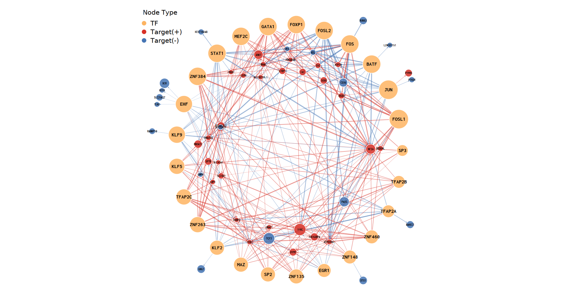

💡 说明：在生成的全局网络图中，请将视线聚焦于被多个 TF 连线交织的内部区域。这些被紧紧包围的“共享靶标”，通常是维持该组织稳态、或处于某条关键信号通路咽喉位置的“命脉基因（Bottleneck Genes）”。而散布在外部放射状边缘的基因，则更多代表了单个 TF 为了维持特定亚群细胞特征而调用的“专属武器库”。此外，观察核心 TF 之间的连线密集程度，还可以帮助您识别出哪些转录因子正在“抱团”发挥协同调控作用。

ATAC + RNA 多组学：Trios 分析 ​

1. 教程简介 ​

2. 输入文件准备 ​

3. 初始三元组构建 ​

3.1 读取 Peak2Gene 结果文件 (Gene2PeakLinks.xls) ​

3.2 加载多组学数据与 Motif-Peak 空间映射 ​

3.3 完成 Trios 初始组装与背景噪音过滤 ​

4. 活跃调控筛选与统计检验 ​

4.1 TF 与靶基因表达相关性计算 (TF-Gene Correlation) ​

4.2 计算 TF 活性与自身表达的一致性相关性 ​

4.3 计算 TF 活性与靶基因表达的相关性 (区分激活与抑制) ​

4.4 综合调控强度评分 (Linkage Score 计算) ​

5. Trios 过滤与高置信度网络输出 ​

6. Trios 可视化 ​

6.1 核心 TF 筛选与靶基因调控散点图 ​

6.2 Trios 调控共变性热图 (Heatmap) ​

6.3 核心 TF 靶基因群的亚群特异性表达热图 ​

6.4 TF-Target 调控网络图 ​

6.5 全局多转录因子协同调控网络图 (Global Regulatory Network) ​