Banksy Spatial Clustering: Principles, Installation, Code Examples, and Interpretation

Author: SeekGene

Time: 16 min

Words: 3.1k words

Updated: 2026-02-28

Reads: 0 times

Spatial-seq Analysis Guide Notebooks Niche Analysis

Load Required R Packages

library(Seurat)
library(Banksy)
library(SummarizedExperiment)
library(SpatialExperiment)
library(scuttle)
library(scater)
library(cowplot)
library(ggplot2)

output

Attaching SeuratObject

Warning message:
“package ‘SummarizedExperiment’ was built under R version 4.3.2”
Loading required package: MatrixGenerics

Warning message:
“package ‘MatrixGenerics’ was built under R version 4.3.3”
Loading required package: matrixStats

Warning message:
“package ‘matrixStats’ was built under R version 4.3.3”

Attaching package: ‘MatrixGenerics’

The following objects are masked from ‘package:matrixStats’:

colAlls, colAnyNAs, colAnys, colAvgsPerRowSet, colCollapse,
colCounts, colCummaxs, colCummins, colCumprods, colCumsums,
colDiffs, colIQRDiffs, colIQRs, colLogSumExps, colMadDiffs,
colMads, colMaxs, colMeans2, colMedians, colMins, colOrderStats,
colProds, colQuantiles, colRanges, colRanks, colSdDiffs, colSds,
colSums2, colTabulates, colVarDiffs, colVars, colWeightedMads,
colWeightedMeans, colWeightedMedians, colWeightedSds,
colWeightedVars, rowAlls, rowAnyNAs, rowAnys, rowAvgsPerColSet,
rowCollapse, rowCounts, rowCummaxs, rowCummins, rowCumprods,
rowCumsums, rowDiffs, rowIQRDiffs, rowIQRs, rowLogSumExps,
rowMadDiffs, rowMads, rowMaxs, rowMeans2, rowMedians, rowMins,
rowOrderStats, rowProds, rowQuantiles, rowRanges, rowRanks,
rowSdDiffs, rowSds, rowSums2, rowTabulates, rowVarDiffs, rowVars,
rowWeightedMads, rowWeightedMeans, rowWeightedMedians,
rowWeightedSds, rowWeightedVars

Loading required package: GenomicRanges

Warning message:
“package ‘GenomicRanges’ was built under R version 4.3.3”
Loading required package: stats4

Loading required package: BiocGenerics

Warning message:
“package ‘BiocGenerics’ was built under R version 4.3.2”

Attaching package: ‘BiocGenerics’

The following objects are masked from ‘package:stats’:

IQR, mad, sd, var, xtabs

The following objects are masked from ‘package:base’:

anyDuplicated, aperm, append, as.data.frame, basename, cbind,
colnames, dirname, do.call, duplicated, eval, evalq, Filter, Find,
get, grep, grepl, intersect, is.unsorted, lapply, Map, mapply,
match, mget, order, paste, pmax, pmax.int, pmin, pmin.int,
Position, rank, rbind, Reduce, rownames, sapply, setdiff, sort,
table, tapply, union, unique, unsplit, which.max, which.min

Loading required package: S4Vectors

Warning message:
“package ‘S4Vectors’ was built under R version 4.3.3”

Attaching package: ‘S4Vectors’

The following object is masked from ‘package:utils’:

findMatches

The following objects are masked from ‘package:base’:

expand.grid, I, unname

Loading required package: IRanges

Warning message:
“package ‘IRanges’ was built under R version 4.3.3”
Loading required package: GenomeInfoDb

Warning message:
“package ‘GenomeInfoDb’ was built under R version 4.3.2”
Loading required package: Biobase

Warning message:
“package ‘Biobase’ was built under R version 4.3.3”
Welcome to Bioconductor

Vignettes contain introductory material; view with
'browseVignettes()'. To cite Bioconductor, see
'citation("Biobase")', and for packages 'citation("pkgname")'.

Attaching package: ‘Biobase’

The following object is masked from ‘package:MatrixGenerics’:

rowMedians

The following objects are masked from ‘package:matrixStats’:

anyMissing, rowMedians

Attaching package: ‘SummarizedExperiment’

The following object is masked from ‘package:SeuratObject’:

Assays

The following object is masked from ‘package:Seurat’:

Assays

Loading required package: SingleCellExperiment

Loading required package: ggplot2

Warning message:
“package ‘ggplot2’ was built under R version 4.3.3”
Warning message:
“package ‘cowplot’ was built under R version 4.3.3”

Read Workflow RDS Data

# Input data here is the Seurat object result file from SeekSpace™ Tools analysis, containing expression matrix and spatial location matrix
obj=readRDS('../../data/AY1739779861133/input.rds')

str(obj, max.level = 2)

output

Formal class 'Seurat' [package "SeuratObject"] with 13 slots
..@ assays :List of 1
..@ meta.data :'data.frame': 32860 obs. of 8 variables:
..@ active.assay: chr "RNA"
..@ active.ident: Factor w/ 16 levels "0","1","2","3",..: 1 2 4 8 3 1 4 4 4 3 ...n .. ..- attr(*, "names")= chr [1:32860] "AAAGGTACGATAACTCGGCACATACAA_1" "AACCACATACAACTCTTGTGATAAGCA_1" "AATGAAGTACCTGACCCCGTGCCGATT_1" "ACGGTCGGCTCTGCCTTTCCTATTAGG_1" ...n ..@ graphs :List of 2
..@ neighbors : list()
..@ reductions :List of 5
..@ images : list()
..@ project.name: chr "SeuratProject"
..@ misc :List of 1
..@ version :Classes 'package_version', 'numeric_version' hidden list of 1
..@ commands :List of 9
..@ tools : list()

# Input here is metadata from SeekSoul™ Online. Banksy analysis doesn't depend on it, but results can be merged into it for SeekSoul™ Online use.
meta=read.table('../../data/AY1739779861133/meta.tsv',header = T, sep = '\t')

head(meta)

A data.frame: 6 × 37
	barcode	orig.ident	nCount_RNA	nFeature_RNA	mito	Sample	raw_Sample	resolution.0.5_d30	mitorelatedgenes	CellAnnotation	⋯	celltype	resolution.1.5_d30	resolution.1.2_d30	Celltype	T_sub	Celltype_new	cluster24	large_celltype	PD1_T	large_celltype_PD1T
	<chr>	<chr>	<int>	<int>	<dbl>	<chr>	<chr>	<int>	<dbl>	<chr>	⋯	<chr>	<int>	<int>	<chr>	<chr>	<chr>	<chr>	<chr>	<chr>	<chr>
1	AAAGGTACGATAACTCGGCACATACAA_1	24110309_T1_T4_T8_expression	200	180	5.0	T8	24110309_T1_T4_T8_expression	0	5.0	B Cell	⋯	Neutrophil	18	12	Macrophage	undefined	B cells	undefined	B_cells	undefined	B_cells
2	AACCACATACAACTCTTGTGATAAGCA_1	24110309_T1_T4_T8_expression	200	175	8.0	T8	24110309_T1_T4_T8_expression	1	8.0	Fibroblast	⋯	Fibroblast	11	4	SMC	undefined	SMC	undefined	SMC	undefined	SMC
3	AATGAAGTACCTGACCCCGTGCCGATT_1	24110309_T1_T4_T8_expression	200	167	11.0	T4	24110309_T1_T4_T8_expression	3	11.0	Tuft Cell	⋯	Tuft Cell	1	1	Epithelial	undefined	Epithelial cells	undefined	Epithelial_cells	undefined	Epithelial_cells
4	ACGGTCGGCTCTGCCTTTCCTATTAGG_1	24110309_T1_T4_T8_expression	200	177	1.0	T1	24110309_T1_T4_T8_expression	7	1.0	T Cell	⋯	T_cells	3	2	T	undefined	T cells	undefined	T_cells	Undefined	T_cells
5	AGACACTCGAACAGTCTAGACCGCCTT_1	24110309_T1_T4_T8_expression	200	185	2.0	T4	24110309_T1_T4_T8_expression	2	2.0	Neutrophil	⋯	Neutrophil	18	12	Macrophage	undefined	B cells	undefined	B_cells	undefined	B_cells
6	AGGAGGTCGAAATGAGTGCACATACAA_1	24110309_T1_T4_T8_expression	200	183	9.5	T8	24110309_T1_T4_T8_expression	0	9.5	B Cell	⋯	B_cell	12	8	B	undefined	B cells	undefined	B_cells	undefined	B_cells

rownames(meta) = meta$barcode
obj@meta.data = meta

Prepare SpatialExperiment Data for Banksy Analysis

colName="Sample"
sample_name="T1"

obj_sample = subset(obj,cells = rownames(obj@meta.data[obj@meta.data[colName] == sample_name,]))
sce <- Seurat::as.SingleCellExperiment(obj_sample)
# spatialCoords is the spatial location matrix of cells.
spatialCoords <- obj_sample@reductions$spatial@cell.embeddings
sample_id <- as.character(obj_sample$Sample)
# Convert to SpatialExperiment object, which serves as input for Banksy
spe <- SpatialExperiment(
    assays = assays(sce),
    rowData = rowData(sce),
    colData = colData(sce),
    sample_id = sample_id,
    spatialCoords = spatialCoords
)

Data Preprocessing

# The commented 4 lines below are for filtering, calculating 5% and 98% quantiles of cell UMI counts, retaining cells within this range. Filtering is not applied by default here.
#qcstats <- perCellQCMetrics(spe)
#thres <- quantile(qcstats$total, c(0.05, 0.98))
#keep <- (qcstats$total > thres[1]) & (qcstats$total < thres[2])
#spe <- spe[, keep]

if (dim(spe)[2] <= 50000) {
    # Use all genes by default. If using all genes, cell count must be under 60000. Data is normalized to median library size.
    spe <- computeLibraryFactors(spe)
    aname <- "normcounts"
    assay(spe, aname) <- normalizeCounts(spe, log = FALSE)

} else {
    # Use highly variable genes
    #' Get HVGs
    seu <- as.Seurat(spe, data = NULL)
    seu <- FindVariableFeatures(seu, nfeatures = 2000)

    #' Normalize data
    scale_factor <- median(colSums(assay(spe, "counts")))
    seu <- NormalizeData(seu, scale.factor = scale_factor, normalization.method = "RC")

    #' Add data to SpatialExperiment and subset to HVGs
    aname <- "normcounts"
    assay(spe, aname) <- GetAssayData(seu)
    spe <- spe[VariableFeatures(seu),]
    
}

Perform Banksy Analysis

AGF and k-geometric parameters determine which surrounding values are used to calculate the neighborhood, using normalized expression (normcounts in se object) to calculate the neighborhood feature matrix. For SeekSpace data, these parameters have relatively small impact; set agf to TRUE and k_geom to c(15, 30).

AGF Parameter

To describe the neighborhood, Banksy calculates weighted neighborhood mean (H_0) and azimuthal Gabor filter (H_1), the latter for estimating gene expression gradients. Setting compute_agf to TRUE computes both H_0 and H_1.

k-geometric Parameter

k_geom specifies the number of neighbors for calculating each H_m (m = 0,1). If a single value is specified, each feature matrix uses the same k_geom. Alternatively, multiple k_geom values can be provided for each feature matrix. Here, we use k_geom[1]=15 and k_geom[2]=30 for H_0 and H_1 respectively. More neighbors are used for gradient calculation.

For datasets generated using Visium v1/v2, use k_geom = 18 (if compute_agf = TRUE, use k_geom <- c(18, 18)), as this corresponds to using two concentric rings of points around each point as the neighborhood.

k_geom <- c(15, 30)
spe <- Banksy::computeBanksy(spe, assay_name = aname, compute_agf = TRUE, k_geom = k_geom)

output

Warning message in asMethod(object):
“sparse->dense coercion: allocating vector of size 1.7 GiB”
Computing neighbors...n
Spatial mode is kNN_median

Parameters: k_geom=15

Done

Computing neighbors...n
Spatial mode is kNN_median

Parameters: k_geom=30

Done

Computing harmonic m = 0

Using 15 neighbors

Done

Computing harmonic m = 1

Using 30 neighbors

Centering

Done

lambda Parameter

Lambda is a mixing parameter in [0,1] determining how much spatial information is included, significantly affecting results. "lambda = 0" corresponds to non-spatial clustering; small "lambda" runs Banksy in cell typing mode; high "lambda" runs Banksy in domain discovery mode. Our goal is domain segmentation, so we generally use larger lambda values. For SeekSpace data, 0.6 or 0.8 yields expected segmentation. In rare cases, if results are irregular with many small regions, try increasing lambda; if regions are too large/coarse, try decreasing it.

Here lambda is set to c(0.6, 0.8), so results for both 0.6 and 0.8 will be calculated and appear in the final cluster results.

lambda <- c(0.6,  0.8)
npcs = 30

set.seed(1000)
spe <- Banksy::runBanksyPCA(spe, use_agf = TRUE,  lambda = lambda, npcs = npcs)
spe <- Banksy::runBanksyUMAP(spe, use_agf = TRUE, lambda = lambda, npcs = npcs)

output

Warning message in asMethod(object):
“sparse->dense coercion: allocating vector of size 1.7 GiB”
Warning message in asMethod(object):
“sparse->dense coercion: allocating vector of size 1.7 GiB”

resolution Parameter

This parameter works like Seurat's res parameter; higher values mean more clusters. Here c(0.4, 0.6) means results for resolution 0.4 and 0.6 will be calculated and appear in the final cluster results.

npcs Parameter

Specifies the number of principal components. Default is 20. If there are many domains, try setting npcs to 50 to increase the final cluster count.

algo Parameter

The algo parameter can be leiden, louvain, kmeans, or mclust.

Leiden and louvain are similar, automatically calculating cluster count, requiring resolution (higher = more clusters). Both yield very "regular" segment domains, with default leiden being the best. Kmeans and mclust are similar, requiring manual cluster count specification. Kmeans segment domains are quite accurate in both mouse brain and human eye data. In summary, start with the default leiden algorithm. If adjusting lambda, npcs, and resolution doesn't yield expected segment domains, try kmeans.

resolution <- c(0.2,0.4)

spe <- Banksy::clusterBanksy(spe, use_agf = TRUE, lambda = lambda, algo = 'leiden', npcs = npcs, resolution = resolution)

When algo is kmeans, use the code below

# If using kmeans clustering, replace the clusterBanksy line above with the commented line below; no other code changes needed.
# se <- Banksy::clusterBanksy(se, use_agf = TRUE, lambda = lambda,  algo = "kmeans", kmeans.centers = c(5,10,15,20,25))

# To visually compare clustering results, use connectClusters to relabel. Run as default, no modification needed.
spe <- Banksy::connectClusters(spe)

output

clust_M1_lam0.8_k50_res0.2 --> clust_M1_lam0.6_k50_res0.2

clust_M1_lam0.8_k50_res0.4 --> clust_M1_lam0.8_k50_res0.2

clust_M1_lam0.6_k50_res0.4 --> clust_M1_lam0.8_k50_res0.4

colnames(colData(spe))

'barcode'
'orig.ident'
'nCount_RNA'
'nFeature_RNA'
'mito'
'Sample'
'raw_Sample'
'resolution.0.5_d30'
'mitorelatedgenes'
'CellAnnotation'
'intestine'
'Group'
'FCN1_LGR5'
'PCDH17_LGR5'
'CD31_LGR5'
'CLDN2_P'
'LGR5_ALL_CELL'
'LGR5_ALL'
'LGR5_ALL_1'
'PCDH17_ALL'
'PCDH17_LGR5_ALL'
'CLDN2_P1'
'FCN1_LGR5_2'
'LGR5_TOTAL'
'CLXCL6_epi'
'CLXCL6_epi_1'
'resolution.1.0_d30'
'celltype'
'resolution.1.5_d30'
'resolution.1.2_d30'
'Celltype'
'T_sub'
'Celltype_new'
'large_celltype'
'PD1_T'
'large_celltype_PD1T'
'ident'
'sample_id'
'sizeFactor'
'clust_M1_lam0.6_k50_res0.2'
'clust_M1_lam0.6_k50_res0.4'
'clust_M1_lam0.8_k50_res0.2'
'clust_M1_lam0.8_k50_res0.4'

Result Visualization

Explanation of cluster labels in the image below, taking "clust_M1_lam0.6_k50_res0.4" as an example:

clust: indicates cluster result

M1: indicates use_agf = TRUE

lam0.6: indicates lambda=0.6

k50: indicates k_neighbors=50, default value, no modification needed

res0.4: indicates resolution=0.4

# Spatial visualization of all clustering labels from Banksy parameter combinations
cnames <- grep("^clust", colnames(colData(spe)), value = TRUE)
colData(spe) <- cbind(colData(spe), spatialCoords(spe))

plots <- list()

for (i in seq_along(cnames)) {
  plots[[i]] <- plotColData(spe, x = "spatial_1", y = "spatial_2", point_size = 1, colour_by = cnames[i]) + coord_equal()
}

options(repr.plot.height=16, repr.plot.width=16)

plot_grid(plotlist = plots, ncol = 2)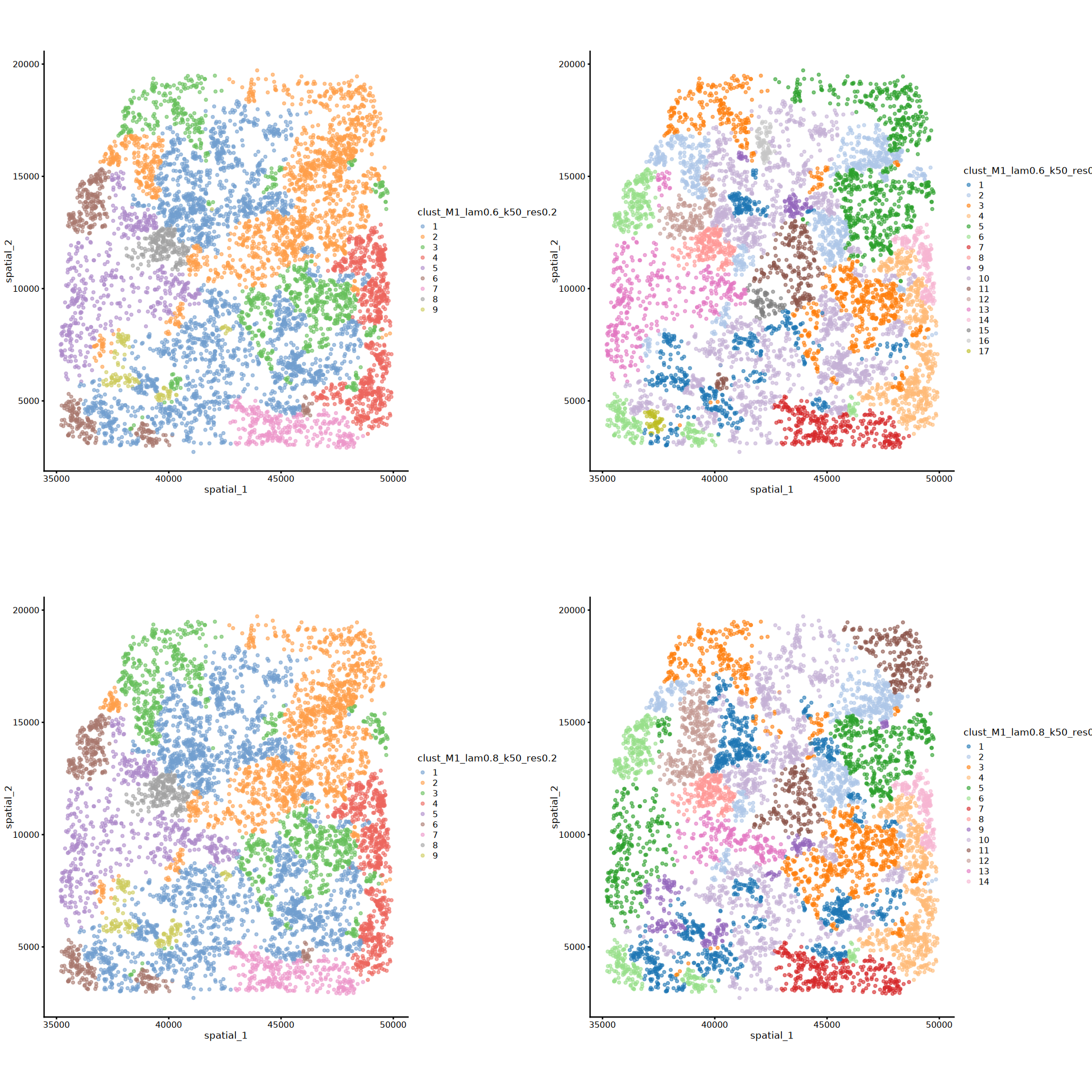

# UMAP visualization of all clustering labels from Banksy parameter combinations
rdnames <- grep("UMAP.*lam", reducedDimNames(spe), value = TRUE)
umap_plots <- list()

plot_num = 1

for (i in seq_along(rdnames)) {
    cnnames_use = cnames[which(grepl(gsub('UMAP_', '', rdnames[i]), cnames))]
    for (j in seq_along(cnnames_use)){
        umap_plots[[plot_num]] <- plotReducedDim(spe, dimred = rdnames[i], colour_by = cnnames_use[j]) +  coord_equal()
        plot_num = plot_num + 1
    } 
}
options(repr.plot.height=16, repr.plot.width=16)
plot_grid(plotlist = umap_plots, ncol = 2)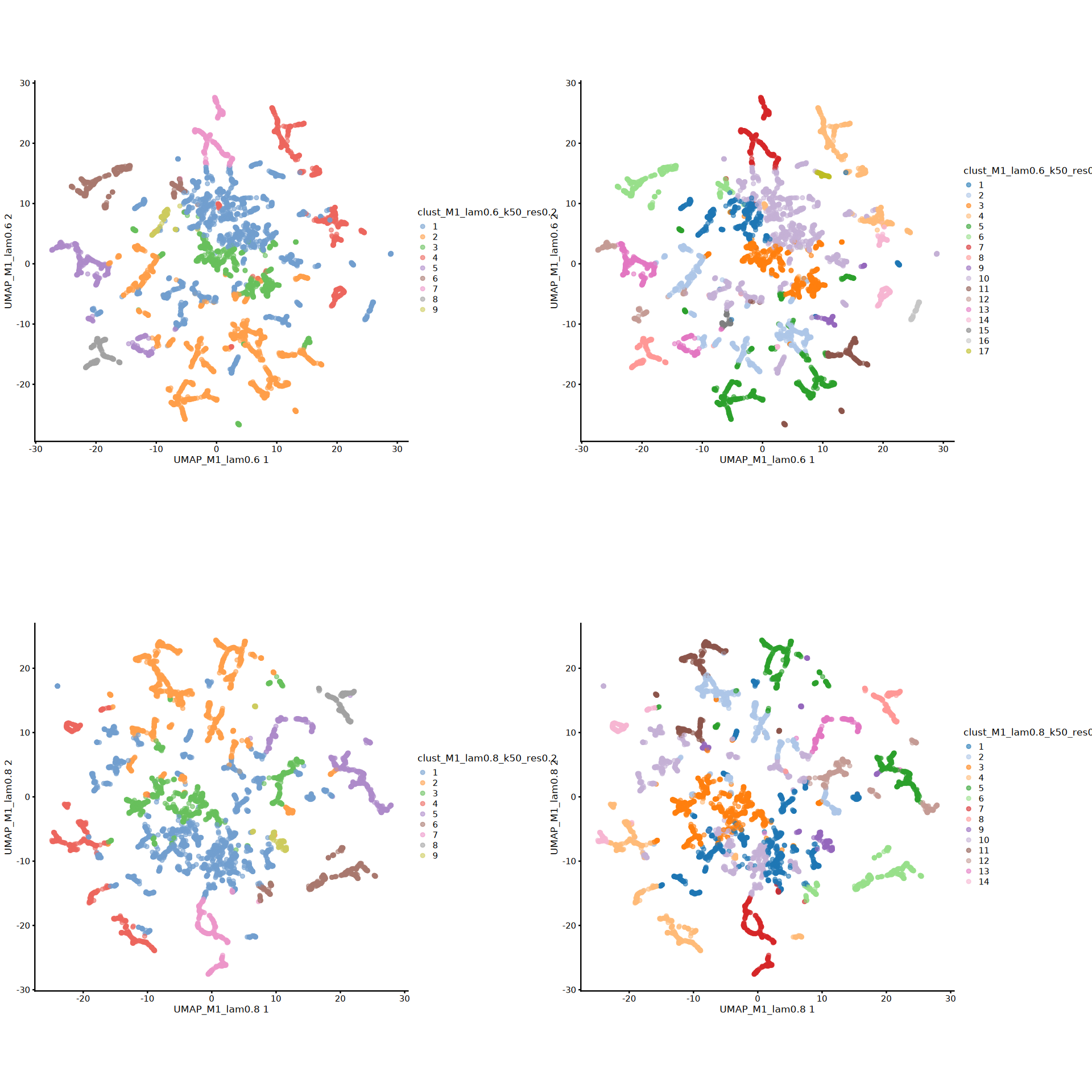

Output Results

# Save Banksy analysis results
save(spe, file='banksy.rda')

# Save Banksy clustering results, which can be merged into Seurat metadata
write.csv(colData(spe), 'banksy_colData.csv')

Banksy Spatial Clustering: Principles, Installation, Code Examples, and Interpretation ​

Load Required R Packages ​

Read Workflow RDS Data ​

Prepare SpatialExperiment Data for Banksy Analysis ​

Data Preprocessing ​

Perform Banksy Analysis ​

Result Visualization ​

Output Results ​

Banksy Spatial Clustering: Principles, Installation, Code Examples, and Interpretation

Load Required R Packages

Read Workflow RDS Data

Prepare SpatialExperiment Data for Banksy Analysis

Data Preprocessing

Perform Banksy Analysis

Result Visualization

Output Results