Banksy 空间聚类:原理、安装、代码示例与结果解读
加载分析需要的 R 包
library(Seurat)
library(Banksy)
library(SummarizedExperiment)
library(SpatialExperiment)
library(scuttle)
library(scater)
library(cowplot)
library(ggplot2)Warning message:
“package ‘SummarizedExperiment’ was built under R version 4.3.2”
Loading required package: MatrixGenerics
Warning message:
“package ‘MatrixGenerics’ was built under R version 4.3.3”
Loading required package: matrixStats
Warning message:
“package ‘matrixStats’ was built under R version 4.3.3”
Attaching package: ‘MatrixGenerics’
The following objects are masked from ‘package:matrixStats’:
colAlls, colAnyNAs, colAnys, colAvgsPerRowSet, colCollapse,
colCounts, colCummaxs, colCummins, colCumprods, colCumsums,
colDiffs, colIQRDiffs, colIQRs, colLogSumExps, colMadDiffs,
colMads, colMaxs, colMeans2, colMedians, colMins, colOrderStats,
colProds, colQuantiles, colRanges, colRanks, colSdDiffs, colSds,
colSums2, colTabulates, colVarDiffs, colVars, colWeightedMads,
colWeightedMeans, colWeightedMedians, colWeightedSds,
colWeightedVars, rowAlls, rowAnyNAs, rowAnys, rowAvgsPerColSet,
rowCollapse, rowCounts, rowCummaxs, rowCummins, rowCumprods,
rowCumsums, rowDiffs, rowIQRDiffs, rowIQRs, rowLogSumExps,
rowMadDiffs, rowMads, rowMaxs, rowMeans2, rowMedians, rowMins,
rowOrderStats, rowProds, rowQuantiles, rowRanges, rowRanks,
rowSdDiffs, rowSds, rowSums2, rowTabulates, rowVarDiffs, rowVars,
rowWeightedMads, rowWeightedMeans, rowWeightedMedians,
rowWeightedSds, rowWeightedVars
Loading required package: GenomicRanges
Warning message:
“package ‘GenomicRanges’ was built under R version 4.3.3”
Loading required package: stats4
Loading required package: BiocGenerics
Warning message:
“package ‘BiocGenerics’ was built under R version 4.3.2”
Attaching package: ‘BiocGenerics’
The following objects are masked from ‘package:stats’:
IQR, mad, sd, var, xtabs
The following objects are masked from ‘package:base’:
anyDuplicated, aperm, append, as.data.frame, basename, cbind,
colnames, dirname, do.call, duplicated, eval, evalq, Filter, Find,
get, grep, grepl, intersect, is.unsorted, lapply, Map, mapply,
match, mget, order, paste, pmax, pmax.int, pmin, pmin.int,
Position, rank, rbind, Reduce, rownames, sapply, setdiff, sort,
table, tapply, union, unique, unsplit, which.max, which.min
Loading required package: S4Vectors
Warning message:
“package ‘S4Vectors’ was built under R version 4.3.3”
Attaching package: ‘S4Vectors’
The following object is masked from ‘package:utils’:
findMatches
The following objects are masked from ‘package:base’:
expand.grid, I, unname
Loading required package: IRanges
Warning message:
“package ‘IRanges’ was built under R version 4.3.3”
Loading required package: GenomeInfoDb
Warning message:
“package ‘GenomeInfoDb’ was built under R version 4.3.2”
Loading required package: Biobase
Warning message:
“package ‘Biobase’ was built under R version 4.3.3”
Welcome to Bioconductor
Vignettes contain introductory material; view with
'browseVignettes()'. To cite Bioconductor, see
'citation("Biobase")', and for packages 'citation("pkgname")'.
Attaching package: ‘Biobase’
The following object is masked from ‘package:MatrixGenerics’:
rowMedians
The following objects are masked from ‘package:matrixStats’:
anyMissing, rowMedians
Attaching package: ‘SummarizedExperiment’
The following object is masked from ‘package:SeuratObject’:
Assays
The following object is masked from ‘package:Seurat’:
Assays
Loading required package: SingleCellExperiment
Loading required package: ggplot2
Warning message:
“package ‘ggplot2’ was built under R version 4.3.3”
Warning message:
“package ‘cowplot’ was built under R version 4.3.3”
读取流程 rds 数据
# 这里输入的数据是 SeekSpace® Tools 分析得到的 Seurat object 结果文件,该 object 包含表达矩阵和空间位置矩阵
obj=readRDS('../../data/AY1739779861133/input.rds')str(obj, max.level = 2)..@ assays :List of 1
..@ meta.data :'data.frame': 32860 obs. of 8 variables:
..@ active.assay: chr "RNA"
..@ active.ident: Factor w/ 16 levels "0","1","2","3",..: 1 2 4 8 3 1 4 4 4 3 ...n .. ..- attr(*, "names")= chr [1:32860] "AAAGGTACGATAACTCGGCACATACAA_1" "AACCACATACAACTCTTGTGATAAGCA_1" "AATGAAGTACCTGACCCCGTGCCGATT_1" "ACGGTCGGCTCTGCCTTTCCTATTAGG_1" ...n ..@ graphs :List of 2
..@ neighbors : list()
..@ reductions :List of 5
..@ images : list()
..@ project.name: chr "SeuratProject"
..@ misc :List of 1
..@ version :Classes 'package_version', 'numeric_version' hidden list of 1
..@ commands :List of 9
..@ tools : list()
# 这里输入的是 SeekSoul Online 上得到的 metadata 文件,Banksy 分析并不依赖这个文件,分析结果可以合并到这个 metadata 中,方便 SeekSoul Online 的使用。
meta=read.table('../../data/AY1739779861133/meta.tsv',header = T, sep = '\t')head(meta)| barcode | orig.ident | nCount_RNA | nFeature_RNA | mito | Sample | raw_Sample | resolution.0.5_d30 | mitorelatedgenes | CellAnnotation | ⋯ | celltype | resolution.1.5_d30 | resolution.1.2_d30 | Celltype | T_sub | Celltype_new | cluster24 | large_celltype | PD1_T | large_celltype_PD1T | |
|---|---|---|---|---|---|---|---|---|---|---|---|---|---|---|---|---|---|---|---|---|---|
| <chr> | <chr> | <int> | <int> | <dbl> | <chr> | <chr> | <int> | <dbl> | <chr> | ⋯ | <chr> | <int> | <int> | <chr> | <chr> | <chr> | <chr> | <chr> | <chr> | <chr> | |
| 1 | AAAGGTACGATAACTCGGCACATACAA_1 | 24110309_T1_T4_T8_expression | 200 | 180 | 5.0 | T8 | 24110309_T1_T4_T8_expression | 0 | 5.0 | B Cell | ⋯ | Neutrophil | 18 | 12 | Macrophage | undefined | B cells | undefined | B_cells | undefined | B_cells |
| 2 | AACCACATACAACTCTTGTGATAAGCA_1 | 24110309_T1_T4_T8_expression | 200 | 175 | 8.0 | T8 | 24110309_T1_T4_T8_expression | 1 | 8.0 | Fibroblast | ⋯ | Fibroblast | 11 | 4 | SMC | undefined | SMC | undefined | SMC | undefined | SMC |
| 3 | AATGAAGTACCTGACCCCGTGCCGATT_1 | 24110309_T1_T4_T8_expression | 200 | 167 | 11.0 | T4 | 24110309_T1_T4_T8_expression | 3 | 11.0 | Tuft Cell | ⋯ | Tuft Cell | 1 | 1 | Epithelial | undefined | Epithelial cells | undefined | Epithelial_cells | undefined | Epithelial_cells |
| 4 | ACGGTCGGCTCTGCCTTTCCTATTAGG_1 | 24110309_T1_T4_T8_expression | 200 | 177 | 1.0 | T1 | 24110309_T1_T4_T8_expression | 7 | 1.0 | T Cell | ⋯ | T_cells | 3 | 2 | T | undefined | T cells | undefined | T_cells | Undefined | T_cells |
| 5 | AGACACTCGAACAGTCTAGACCGCCTT_1 | 24110309_T1_T4_T8_expression | 200 | 185 | 2.0 | T4 | 24110309_T1_T4_T8_expression | 2 | 2.0 | Neutrophil | ⋯ | Neutrophil | 18 | 12 | Macrophage | undefined | B cells | undefined | B_cells | undefined | B_cells |
| 6 | AGGAGGTCGAAATGAGTGCACATACAA_1 | 24110309_T1_T4_T8_expression | 200 | 183 | 9.5 | T8 | 24110309_T1_T4_T8_expression | 0 | 9.5 | B Cell | ⋯ | B_cell | 12 | 8 | B | undefined | B cells | undefined | B_cells | undefined | B_cells |
rownames(meta) = meta$barcode
obj@meta.data = meta
准备 Banksy 分析所需的 SpatialExperiment 格式数据
colName="Sample"
sample_name="T1"obj_sample = subset(obj,cells = rownames(obj@meta.data[obj@meta.data[colName] == sample_name,]))
sce <- Seurat::as.SingleCellExperiment(obj_sample)
# spatialCoords为细胞的空间位置矩阵。
spatialCoords <- obj_sample@reductions$spatial@cell.embeddings
sample_id <- as.character(obj_sample$Sample)
# 转为SpatialExperiment对象,该对象作为banksy的输入
spe <- SpatialExperiment(
assays = assays(sce),
rowData = rowData(sce),
colData = colData(sce),
sample_id = sample_id,
spatialCoords = spatialCoords
)数据前处理
# 下面注释的4行代码是做过滤用的,计算细胞umi counts的 5%和 98%分位数,只保留umi总数在这个分位数中间的细胞。这里默认没有做过滤。
#qcstats <- perCellQCMetrics(spe)
#thres <- quantile(qcstats$total, c(0.05, 0.98))
#keep <- (qcstats$total > thres[1]) & (qcstats$total < thres[2])
#spe <- spe[, keep]

if (dim(spe)[2] <= 50000) {
    # 默认使用全部基因,如果使用全部基因,细胞数必需在60000以内,将数据归一化为平局文库大小
    spe <- computeLibraryFactors(spe)
    aname <- "normcounts"
    assay(spe, aname) <- normalizeCounts(spe, log = FALSE)

} else {
    # 使用高变基因
    #' Get HVGs
    seu <- as.Seurat(spe, data = NULL)
    seu <- FindVariableFeatures(seu, nfeatures = 2000)

    #' Normalize data
    scale_factor <- median(colSums(assay(spe, "counts")))
    seu <- NormalizeData(seu, scale.factor = scale_factor, normalization.method = "RC")

    #' Add data to SpatialExperiment and subset to HVGs
    aname <- "normcounts"
    assay(spe, aname) <- GetAssayData(seu)
    spe <- spe[VariableFeatures(seu),]

}
进行 Banksy 分析
AGF 和 k-geometric 两个参数决定了采用周围哪些值来计算邻域,计算的时候使用归一化表达(se 对象中的 normcounts)来计算邻域特征矩阵。对于 SeekSpace 数据,这两个参数对结果的影响相对较小,agf 设为 TURE,k_geom 值为 c(15, 30)。
- AGF 参数
为了描述邻域,Banksy 计算加权邻域均值(H_0)和方位角 Gabor 滤波器(H_1),后者用于估计基因表达梯度。将 compute_agf 设置为 TRUE 会同时计算 H_0 和 H_1。
- k-geometric 参数
k_geom 指定用于计算每个 H_m(m = 0,1)的邻居数量。如果指定单个值,那么每个特征矩阵将使用相同的 k_geom。或者,可以为每个特征矩阵提供多个 k_geom 值。在这里,我们对 H_0 和 H_1 分别使用 k_geom [1]=15 和 k_geom [2]=30。更多的邻居被用于计算梯度。
对于使用 Visium v1/v2 生成的数据集,使用 k_geom = 18(如果 compute_agf = TRUE,则使用 k_geom <- c (18, 18)),因为这对应于将每个点周围的两个同心环的点作为邻域。
k_geom <- c(15, 30)
spe <- Banksy::computeBanksy(spe, assay_name = aname, compute_agf = TRUE, k_geom = k_geom)“sparse->dense coercion: allocating vector of size 1.7 GiB”
Computing neighbors...n
Spatial mode is kNN_median
Parameters: k_geom=15
Done
Computing neighbors...n
Spatial mode is kNN_median
Parameters: k_geom=30
Done
Computing harmonic m = 0
Using 15 neighbors
Done
Computing harmonic m = 1
Using 30 neighbors
Centering
Done
- lambda 参数
lambda 是一个取值在 [0,1] 区间的混合参数,它决定了在下游分析中纳入多少空间信息,对结果影响较大。当“lambda = 0”,它对应于非空间聚类;当 “lambda” 值较小时,BANKY 在细胞分型模式下运行;当 “lambda” 值较高时,Banksy 在区域发现模式下运行。我们这里的分析目的,还是要得到区域分割的结果,所以一般使用较大的 lambda 值。对于 SeekSpace 数据,使用 0.6 或者 0.8 都可以得到符合预期的区域分割结果。少数情况下,如果发现结果不规整,出现较多小的区域时,可以尝试大的 lambda 值;如果发现区域分割的太大,区域不够精细时,可以尝试调小该值。
这里 lambda 取值 c(0.6, 0.8),则会计算当 lamda=0.6 和 0.8 两个值的结果,两个结果均会出现在最终的 cluster 结果中。
lambda <- c(0.6,  0.8)
npcs = 30

set.seed(1000)
spe <- Banksy::runBanksyPCA(spe, use_agf = TRUE,  lambda = lambda, npcs = npcs)
spe <- Banksy::runBanksyUMAP(spe, use_agf = TRUE, lambda = lambda, npcs = npcs)“sparse->dense coercion: allocating vector of size 1.7 GiB”
Warning message in asMethod(object):
“sparse->dense coercion: allocating vector of size 1.7 GiB”
- resolution 参数
该参数的作用与 Seurat 的 res 参数的作用是类似的,该值越大,则 cluster 越多。这里取值 c(0.4, 0.6),将分别计算 resolution 为 0.4 和 0.6 时的结果,结果均会出现在最终的 cluster 结果中。
- npcs 参数
指定要使用的主成分数量。默认值是 20,如果 domain 比较多,可以尝试将 npcs 设置为 50,来增加最终的 clsuter 数目。
- algo 参数
algo 参数的值可以是 leiden,louvain,kmeans 或者 mclust。
leiden 和 louvain 是相似的算法,都自动计算 cluster 数量,需要指定 resolution,resolution 越高,分的群越多。这两种算法得到 segment domain 非常“规整”,尤其是默认的 leiden 是最好的。 kmean 和 mclsut 是相似的算法,都需要手动来指定 clsuter 的数量,最终结果中 clsuter 也是按照指定的数量来呈现的。kmeans 的 segment domain 分的挺准确的,无论在小鼠脑和人眼数据中。 总的来说,可以首先使用默认的 leiden 算法,如果通过调整 lamda,npcs 和 resolution 参数,无法得到预期的 segment domain,再用 kmeans 试一下。
resolution <- c(0.2,0.4)

spe <- Banksy::clusterBanksy(spe, use_agf = TRUE, lambda = lambda, algo = 'leiden', npcs = npcs, resolution = resolution)
当 algo 选择 kmeans,则用下面代码
# 如果使用kmeans聚类,则将上面clusterBanksy行的代码,替换为下面注释掉的这行代码即可,无需修改教程的其他代码。
# se <- Banksy::clusterBanksy(se, use_agf = TRUE, lambda = lambda, algo = "kmeans", kmeans.centers = c(5,10,15,20,25))# 为了直观地比较聚类运行结果,可以使用 connectClusters,给结果新的标签。默认运行即可,无需修改。
spe <- Banksy::connectClusters(spe)clust_M1_lam0.8_k50_res0.4 --> clust_M1_lam0.8_k50_res0.2
clust_M1_lam0.6_k50_res0.4 --> clust_M1_lam0.8_k50_res0.4
colnames(colData(spe))- 'barcode'
- 'orig.ident'
- 'nCount_RNA'
- 'nFeature_RNA'
- 'mito'
- 'Sample'
- 'raw_Sample'
- 'resolution.0.5_d30'
- 'mitorelatedgenes'
- 'CellAnnotation'
- 'intestine'
- 'Group'
- 'FCN1_LGR5'
- 'PCDH17_LGR5'
- 'CD31_LGR5'
- 'CLDN2_P'
- 'LGR5_ALL_CELL'
- 'LGR5_ALL'
- 'LGR5_ALL_1'
- 'PCDH17_ALL'
- 'PCDH17_LGR5_ALL'
- 'CLDN2_P1'
- 'FCN1_LGR5_2'
- 'LGR5_TOTAL'
- 'CLXCL6_epi'
- 'CLXCL6_epi_1'
- 'resolution.1.0_d30'
- 'celltype'
- 'resolution.1.5_d30'
- 'resolution.1.2_d30'
- 'Celltype'
- 'T_sub'
- 'Celltype_new'
- 'large_celltype'
- 'PD1_T'
- 'large_celltype_PD1T'
- 'ident'
- 'sample_id'
- 'sizeFactor'
- 'clust_M1_lam0.6_k50_res0.2'
- 'clust_M1_lam0.6_k50_res0.4'
- 'clust_M1_lam0.8_k50_res0.2'
- 'clust_M1_lam0.8_k50_res0.4'
结果可视化
对下面图片中 cluster 的标签的意义,做一下解释,以“clust_M1_lam0.6_k50_res0.4”为例:
clust,代表是 cluster 结果
M1,代表 use_agf = TRUE
lam0.6,代表 lambda=0.6
k50,代表 k_neighbors=50,该值为默认值,无需修改
res0.4,代表 resolution=0.4
# banksy各参数组合分析得到的所有聚类标签下的空间可视化
cnames <- grep("^clust", colnames(colData(spe)), value = TRUE)
colData(spe) <- cbind(colData(spe), spatialCoords(spe))

plots <- list()

for (i in seq_along(cnames)) {
  plots[[i]] <- plotColData(spe, x = "spatial_1", y = "spatial_2", point_size = 1, colour_by = cnames[i]) + coord_equal()
}

options(repr.plot.height=16, repr.plot.width=16)

plot_grid(plotlist = plots, ncol = 2)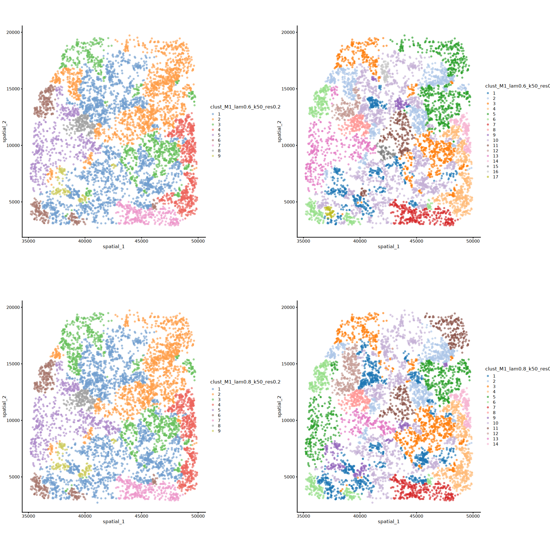
# banksy各参数组合分析得到的所有聚类标签下的UMAP可视化
rdnames <- grep("UMAP.*lam", reducedDimNames(spe), value = TRUE)
umap_plots <- list()

plot_num = 1

for (i in seq_along(rdnames)) {
    cnnames_use = cnames[which(grepl(gsub('UMAP_', '', rdnames[i]), cnames))]
    for (j in seq_along(cnnames_use)){
        umap_plots[[plot_num]] <- plotReducedDim(spe, dimred = rdnames[i], colour_by = cnnames_use[j]) +  coord_equal()
        plot_num = plot_num + 1
    }
}
options(repr.plot.height=16, repr.plot.width=16)
plot_grid(plotlist = umap_plots, ncol = 2)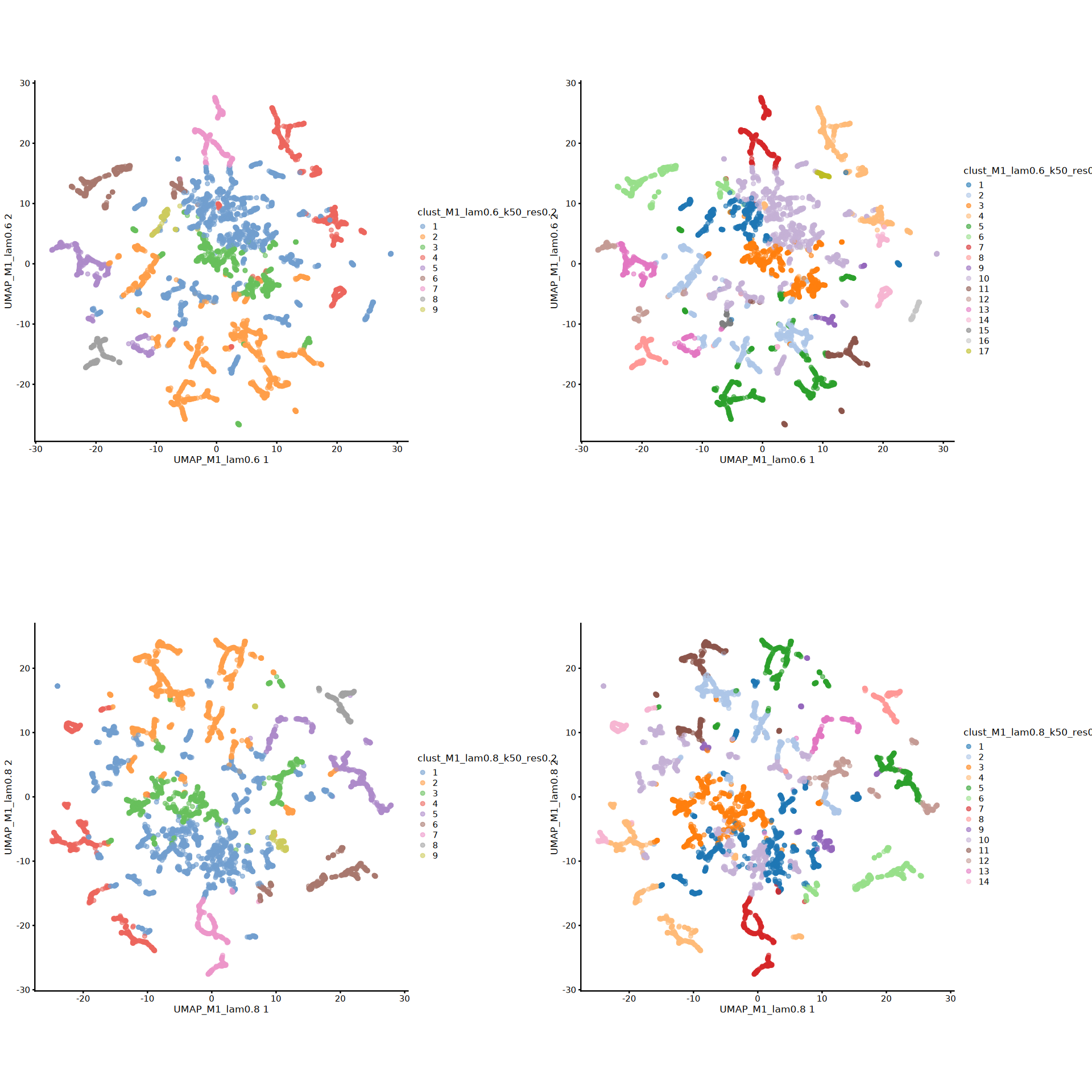
输出结果
# 保存banksy的分析结果
save(spe, file='banksy.rda')# 保存banksy分析得到的聚类结果,这个结果可以合并到seurat的metadata中
write.csv(colData(spe), 'banksy_colData.csv')