epiAneufinder Analysis: Aneuploidy Detection Based on scATAC-seq
Background
Chromosomal Copy Number Variation (CNV) is a hallmark of tumor genome instability, characterized by large-scale amplification or deletion of chromosomal segments. CNV drives tumorigenesis, progression, and therapeutic resistance by altering copy numbers of oncogenes (e.g., MYC) or tumor suppressors (e.g., TP53) through gene dosage effects. Resolving CNV at single-cell resolution is crucial for revealing tumor heterogeneity: using malignant cell-specific CNV profiles (e.g., chromosome 7 amplification, chromosome 10 deletion), one can distinguish tumor cells from non-malignant cells (e.g., T cells, fibroblasts) in complex microenvironments and further resolve subclonal structures and their epigenetic regulatory differences.
Compared to scRNA-seq-based CNV inference, scATAC-seq uses genomic coverage as a direct signal, unaffected by transcriptional programs and transient expression fluctuations; it also has more uniform coverage in non-transcribed regions, thus offering higher resolution and robustness for large-segment and fine-grained CNV. epiAneufinder is a tool specifically for inferring CNV from scATAC-seq data, using coverage counts in fixed genomic windows as proxy signals for DNA copy status to identify chromosomal amplification/deletion events at the single-cell level, thereby enabling differentiation of malignant vs. non-malignant cells and fine characterization of subclones.
Purpose and Significance
- Cell-level Tumor Identification: Accurately distinguish malignant cells from microenvironmental cells based on CNV profiles.
- Subclonal Heterogeneity Resolution: Reconstruct copy number evolutionary trajectories to understand clonal competition and differentiation.
- Multi-omics Integrated Interpretation: Integrate CNV with chromatin accessibility and cell annotation/clustering results to elucidate the impact of genomic structural changes on epigenetic regulation and cell state.
- Clinical Translational Value: Provide structural variation evidence for prognosis stratification, efficacy assessment, and potential target mining.
Parameter Settings
Please first mount the cloud platform pipeline data to be analyzed; refer to Jupyter usage tutorial for mounting instructions
Specific parameter entry:
- meta: Mounted pipeline-related meta file, which is the meta.data inside the pipeline-related Seurat object;
- species: Species information, supports human and mouse only;
- celltype_col: Cell type column name, select the label corresponding to the cell type or cluster to be analyzed. If analyzing annotated cell types, select their corresponding label, e.g., CellAnnotation;
- resolution_cluster: Cell type, multiple selection, select cell type or clustering result to analyze, e.g., Monocyte and Macrophage;
- file_path: fragment file of sample to be analyzed, supports multiple samples;
- SAMplenames: Sample names, supports multiple samples.
# Parameters
meta = "/PROJ2/FLOAT/advanced-analysis/test/2388-5504-5323-570556340787763834/meta.txt"
species = "human"
celltype_col = "CellAnnotation"
resolution_cluster = "wknn_res.0.5_d30_l2_50"
file_path=c("/PROJ2/FLOAT/advanced-analysis/test/2388-5504-6345-581728456711101050/joint14_A_fragments.tsv.gz","/PROJ2/FLOAT/advanced-analysis/test/2388-5504-6345-581728456711101050/joint22_A_fragments.tsv.gz")
samplenames = c("joint14","joint22")# Conditional logic, load species info
if (species == "human") {
genome <- "BSgenome.Hsapiens.UCSC.hg38"
blacklist <- "/PROJ2/FLOAT/shumeng/project/scATAC_learn/Signac/epiAneufinder/bin/hg38-blacklist.v2.bed"
} else if (species == "mouse") {
genome <- "BSgenome.Mmusculus.UCSC.mm10"
blacklist <- "/PROJ2/FLOAT/shumeng/project/scATAC_learn/Signac/epiAneufinder/bin/mm10-blacklist.v2.bed"
} else {
stop(paste0("Unsupported species '", species, "'. Supported: human, mouse."))
}Environment Preparation
Load R Packages
Please select the 'common_r' environment for this integration tutorial
options(warn = -1)
suppressWarnings({
  suppressMessages({
  Sys.setenv(R_DATATABLE_MMAP = "false")
  library(data.table)
  library(epiAneufinder,lib.loc="/PROJ2/FLOAT/shumeng/apps/miniconda3/envs/epiAneufinderR4.3.3/lib/R/library")
  library(RColorBrewer)
  library(Seurat)
  library(ComplexHeatmap)
    })
})
options(warn = 0)colors <- unique(c('#E5D2DD', '#53A85F', '#F1BB72', '#F3B1A0', '#D6E7A3', '#57C3F3', '#476D87',
'#E95C59', '#E59CC4', '#AB3282', '#23452F', '#BD956A', '#8C549C', '#585658',
'#9FA3A8', '#E0D4CA', '#5F3D69', '#C5DEBA', '#58A4C3', '#E4C755', '#F7F398',
'#AA9A59', '#E63863', '#E39A35', '#C1E6F3', '#6778AE', '#91D0BE', '#B53E2B',
'#712820', '#DCC1DD', '#CCE0F5', '#CCC9E6', '#625D9E', '#68A180', '#3A6963',
'#968175', "#6495ED", "#FFC1C1",'#f1ac9d','#f06966','#dee2d1','#6abe83','#39BAE8','#B9EDF8','#221a12',
'#b8d00a','#74828F','#96C0CE','#E95D22','#017890','#F1BB72', '#D6E7A3', '#57C3F3', '#476D87',
'#E95C59', '#E59CC4', '#AB3282', '#BD956A', '#8C549C', '#585658',
'#9FA3A8', '#E0D4CA', '#5F3D69', '#C5DEBA', '#58A4C3', '#E4C755', '#F7F398',
'#AA9A59', '#E63863', '#E39A35', '#C1E6F3', '#6778AE', '#91D0BE', '#B53E2B',
'#712820', '#DCC1DD', '#CCE0F5', '#CCC9E6'))Fragment File Preprocessing
Fragments files generated by SeekArctools or cellranger arc/ATAC contain fragment information for all barcodes, only some of which are real cells. To save computational resources and maintain consistency with downstream cell annotation, filter fragments before CNV analysis: retain only "cell whitelist" barcodes that passed QC and are used for downstream analysis. It is recommended to subset fragments based on established cell metadata/annotation tables (e.g., list of barcodes passing QC and included in analysis) to avoid introducing low-quality barcodes or non-cell background noise into CNV inference.
meta <- read.table(meta,sep="\t",header=T)  # Read mounted meta file containing barcode info for all samples
Barcodes <- meta$barcodes # Extract all Barcodes
# Build a merged_filtered_fragments.tsv file to facilitate continuous output of processed content after processing each sample fragment file sequentially
output_file <- "./merged_filtered_fragments.tsv"

# Write column names outside the loop first (skip this step if column names are not needed)
write.table(t(c("chr", "start", "end", "Barcode", "reads")),
            file = output_file,
            quote = FALSE,
            row.names = FALSE,
            col.names = FALSE,
            sep = "\t")

# Modify loop
for(sample in samplenames){
    file_path <- grep(pattern = sample, file_paths, value = TRUE) # Note this should be file_paths (plural)
    frag <- fread(file_path, header=F)

    # Fix column name assignment syntax error here
    colnames(frag) <- c("chr", "start", "end", "Barcode", "reads") # Use <- for assignment

    frag_filter <- frag[Barcode %in% Barcodes]

    # Append to the same file, append = TRUE is a key parameter
    write.table(frag_filter,
                file = output_file,
                quote = FALSE,
                row.names = FALSE,
                col.names = FALSE, # Do not write column names to avoid duplication
                sep = "\t",
                append = TRUE)     # Append mode, not overwrite
}
Start CNV Analysis
Start executing the epiAneufinder CNV inference workflow. This workflow converts scATAC-seq fragment data into a genome-wide fixed-window coverage matrix, and resolves chromosomal copy number variations at the single-cell level through noise control and event identification.
Execution Steps Overview:
- Data Preprocessing: Load corresponding genome and blacklist files based on species information, set window size (100 kb) and filtering parameters
- CNV Inference: Call epiAneufinder core functions to perform binning counting, noise filtering, and event identification
- Result Output: Generate a matrix table containing CNV states for each window, supporting subsequent visualization and cell clustering integration
Key Parameter Description:
- Window Size: Default 100 kb, balancing CNV resolution and statistical robustness
- Cell Filtering: minFrags=20000, ensuring cell coverage meets CNV inference requirements
- Event Identification: k=4 clustering parameter, minsize=1 minimum event length, threshold_blacklist_bins=0.85 blacklist threshold
- Chromosome Exclusion: Automatically exclude chrX/Y/M to avoid interference from sex and mitochondrial differences
options(future.globals.maxSize=100*1024^3)
invisible(capture.output(
  suppressMessages(
      epiAneufinder::epiAneufinder(input = output_file,# The input fragment file is the fragment file processed and merged in the previous step
                                 outdir = "./",
                                 blacklist = blacklist,
                                 windowSize = 1e5,
                                 genome = genome,
                                 exclude = c('chrX', 'chrY', 'chrM'),
                                 reuse.existing = TRUE,
                                 uq = 0.9,
                                 lq = 0.1,
                                 title_karyo = "Karyoplot",
                                 ncores = 4,
                                 minFrags = 20000,
                                 minsize = 1,
                                 k = 4,
                                 threshold_blacklist_bins = 0.85,
                                 minsizeCNV = 0
                                  )
  )
)
         )
Process Result Files
Process the above CNV analysis result file (../result/epiAneufinder_results/results_table.tsv) for visualization
meta <- meta[,c("barcodes",celltype_col,resolution_cluster)]
colnames(meta)[1] <- "cell"
colnames(meta)[2] <- "annot"
meta$cell <- paste0("cell-",meta$cell)
res_table <- read.table("./epiAneufinder_results/results_table.tsv", header = T,check.names = FALSE)
meta <- meta[which(meta$cell %in% colnames(res_table)),]
rownames(meta) <- meta$cell
res_table <- as.data.frame(res_table)
rownames(res_table) <- paste0(res_table$seq, ":", res_table$start, "-", res_table$end)
res_table <- res_table[,-c(1,2,3)]
res_table <- t(res_table)
chr <- colnames(res_table)
colann <- data.frame(
  chromosome = stringr::str_split(chr, ":", simplify = TRUE)[,1],
  position = stringr::str_split(chr, ":", simplify = TRUE)[,2]
)
rownames(colann) <- paste0(colann$chromosome,":",colann$position)
colann$chromosome <- gsub("chr", "", colann$chromosome)
Heatmap Visualization
Visualize cell copy number variations using a heatmap. Copy number values around 2 indicate normal diploidy; values between 1 and 2 indicate chromatin deletion, closer to 1 means more severe deletion; values between 2 and 3 indicate chromatin amplification, closer to 3 means more severe amplification. The color bar on the left of the heatmap indicates cell arrangement by cell type and clustering. Each row represents a cell, each column represents a chromosome arm. Heatmap colors represent CNV scores, redder indicates more severe amplification, bluer indicates more severe deletion.
# Dynamically generate colors (keep original code unchanged)
n_clusters <- length(unique(meta[[resolution_cluster]]))
clusters_colors  <- sample(colors, n_clusters, replace = FALSE)
n_celltypes <- length(unique(meta$annot))
cell_type_colors  <- sample(colors, n_celltypes, replace = FALSE)
# Optimized annotation code
ha <- rowAnnotation(
    Cell_type = meta$annot,
    Cluster = meta[[resolution_cluster]],
    col = list(
        Cluster = setNames(clusters_colors, unique(meta[[resolution_cluster]])),
        Cell_type = setNames(cell_type_colors, unique(meta$annot))
    ),
    annotation_label = list(
        Cluster = "Cluster",
        Cell_type = "Cell Type"
    ),
    annotation_name_gp = gpar(fontsize = 8),
    annotation_name_rot = 45,
    annotation_legend_param = list(
        Cluster = list(labels_gp = gpar(fontsize = 10)),
        Cell_type = list(labels_gp = gpar(fontsize = 10))
    ),
    width = unit(10, "cm")
)ht_opt$message = FALSE
p <- Heatmap(
res_table,
name = "Copy Number",
left_annotation = ha, # Uncomment and ensure ha is defined
show_row_names = FALSE,
show_column_names = FALSE,
cluster_rows = TRUE,
cluster_columns = FALSE,
row_split = meta[,2],
row_title = "Cell Type",
column_split = factor(colann[,1],levels = c(1:22)), # Use corrected grouping
column_gap = unit(1, "mm"), # Control divider gap
cluster_row_slices = FALSE,
use_raster = TRUE,
show_row_dend = FALSE,
border = FALSE
)options(repr.plot.height=10, repr.plot.width=15)
invisible(pdf("../result/cnv_heatmap_annotated.pdf", width = 15, height = 10))
invisible(draw(p))
invisible(dev.off())
draw(p)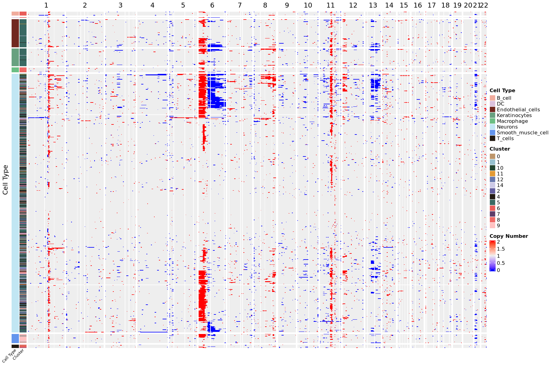
Heatmap Visualization
Visualize cell copy number variations with a heatmap. Copy number values around 2 indicate normal diploidy; values between 1 and 2 indicate chromatin deletion, with values closer to 1 indicating more severe deletion; values between 2 and 3 indicate chromatin amplification, with values closer to 3 indicating more severe amplification.
The above is a heatmap visualization of chromosomal copy number variations. The color bar on the left of the heatmap indicates cell arrangement by cell type and clustering. Each row represents a cell, each column represents a chromosome arm. Heatmap colors represent CNV scores, redder indicates more severe amplification, bluer indicates more severe deletion.Result Files
├── ./epiAneufinder_results/karyo_annotated.pngcnv_plots
Result Directory: Directory includes all images and tables involved in this analysis
Literature Case Analysis
《The chromatin landscape of high-grade serous ovarian cancer metastasis identifies regulatory drivers in post-chemotherapy residual tumour cells》
In this study, the authors used epiAneufinder for copy number variation analysis on scATAC-seq to distinguish tumor cells from non-tumor cells
References
[1] Nikolic A, Singhal D, Ellestad K, et al.Copy-scAT: Deconvoluting single-cell chromatin accessibility of genetic subclones in cancer[J].Science advances, 2021, 7(42):eabg6045.DOI: 10.1126/sciadv.abg6045.
Appendix
.txt: Result data table files, tab-separated. Unix/Linux/Mac users use less or more commands to view; Windows users use advanced text editors like Notepad++ to view, or open with Microsoft Excel.
.pdf: Result image files, vector graphics, can be zoomed in and out without distortion, convenient for users to view and edit, can use Adobe Illustrator for image editing, used for article publication, etc.
.rds: Seurat object containing gene activity assay, needs to be opened in R environment for viewing and further analysis.