scMethyl + RNA Multi-omics: Differential Analysis and Functional Enrichment Analysis

Author: SeekGene

Time: 82 min

Words: 16.6k words

Updated: 2026-03-18

Reads: 0 times

scMethyl + RNA-seq Notebooks

Module Introduction

This module integrates two core workflows: Single-cell Methylation Differential Analysis and Functional Enrichment Analysis, aiming to identify differentially methylated regions/genes and differentially expressed genes from single-cell multi-omics data, and further analyze their biological functions.

Analysis Overview

Part 1: Differential Analysis

• DMB (Differentially Methylated Bins): Analysis of differentially methylated bins, identifying genomic regions (20 kb windows) with significant differences in methylation levels between different cell types.
• DEG (Differentially Expressed Genes): Analysis of differentially expressed genes, identifying genes with significant differences in expression levels between different cell types.
• DMG (Differentially Methylated Genes): Analysis of differentially methylated genes, identifying genes with significant differences in methylation levels between different cell types (gene region ±2 kb).
• Multi-omics Association Analysis: Integrating transcriptome and methylation data to reveal regulatory relationships between epigenetic modifications and gene expression using Venn diagrams and Circos plots.

Part 2: Functional Enrichment Analysis

• GO Enrichment Analysis: Based on the Gene Ontology (GO) database, identifying biological processes (BP), molecular functions (MF), and cellular components (CC) enriched by differential genes.
• KEGG Enrichment Analysis: Based on the KEGG pathway database, identifying biological pathways enriched by differential genes.

Technical Features

• Statistical Methods: Using Wilcoxon Rank-Sum test for differential analysis, with multiple comparison correction (FDR) to control the false discovery rate.
• Automated Workflow: Integrating data preprocessing, differential analysis, functional enrichment, and visualization.
• Multi-omics Integration: Analyzing transcriptome and methylation data simultaneously to reveal epigenetic regulatory mechanisms.

💡 Note
This analysis workflow applies to single-cell multi-omics data with completed cell type annotation, requiring both transcriptome (RNA) and methylation data.

Input File Preparation

Required Files

This module requires the following input files:

File Type	File Format	Required Columns/Attributes	Description
Transcriptome Data	*.h5ad	obs['celltype'], var['gene_ids']	Annotated transcriptome data containing cell type information and gene IDs
Methylation Data	*.h5ad	obs['celltype'], obs['Sample']	Annotated methylation data containing cell type and sample information
MCDS Data	*.mcds	chrom20k, geneslop2k	Multi-sample MCDS data containing methylation information for 20 kb windows and gene regions ±2 kb

File Structure Requirements

Directory Structure Example:

data/
├── AY1768874914782
│   └── methylation
│       └── demoWTJW969-task-1
│           └── WTJW969
│               ├── allcools_generate_datasets
│               │   └── WTJW969.mcds # Methylation data
│               ├── filtered_feature_bc_matrix # Transcriptome expression matrix
│               └── split_bams
│                   ├── WTJW969_cells.csv
│                   └── filtered_barcode_reads_counts.csv
└── AY1768876253533
    └── methylation
        └── demo4WTJW880-task-1
            └── WTJW880
                ├── allcools_generate_datasets
                │   └── WTJW880.mcds # Methylation data
                ├── filtered_feature_bc_matrix # Transcriptome expression matrix
                └── split_bams
                    ├── WTJW880_cells.csv
                    └── filtered_barcode_reads_counts.csv

Data Preprocessing Requirements

1. Complete Annotation: Transcriptome and methylation data must contain complete cell type annotations (celltype column).
2. QC Completed: Transcriptome data needs to be normalized.
3. MCDS Preparation: MCDS data needs to contain chrom20k and geneslop2k dimensions.

⚠️ Important Note
Missing annotation information will prevent subsequent analysis. Please ensure all required columns exist and are formatted correctly.

import os
import re
import glob
from ALLCools.mcds import MCDS
from ALLCools.clustering import tsne, significant_pc_test, log_scale, lsi, binarize_matrix, filter_regions, cluster_enriched_features, ConsensusClustering, Dendrogram, get_pc_centers
from ALLCools.clustering.doublets import MethylScrublet
from ALLCools.plot import *
import scanpy as sc
import numpy as np
import pandas as pd
import matplotlib.pyplot as plt
import matplotlib.colors as mcolors
from matplotlib.lines import Line2D
import warnings
import xarray as xr
from ALLCools.clustering import one_vs_rest_dmg
import pybedtools
from scipy import sparse
from pycirclize import Circos
from pycirclize.utils import load_eukaryote_example_dataset

# Functional enrichment analysis related packages
import sys
import subprocess
from pathlib import Path
import gseapy as gp
from gseapy import barplot, dotplot
from IPython.display import display, HTML

# Differential analysis parameters
samples = ["WTJW969", "WTJW880"]
sample_path_config = {
    "WTJW969": {"top_dir": "AY1768874914782", "demo_dir": "demoWTJW969-task-1"},
    "WTJW880": {"top_dir": "AY1768876253533", "demo_dir": "demo4WTJW880-task-1"}
}
anno_col = 'celltype'  # Cell type annotation column name

# Functional enrichment analysis parameters
species = "human"  # Species: 'human' or 'mouse'
deg_file = "DEG.csv"  # Differential expression gene file path
dmg_file = "DMG.csv"  # Differential methylation gene file path
output_dir = "./enrichment_results/"  # Enrichment analysis result output directory

## Plotting palette
my_palette = [
    "#66C2A5", "#FC8D62", "#8DA0CB", "#E78AC3", 
    "#A6D854", "#FFD92F", "#E5C494", "#B3B3B3", 
    "#8DD3C7", "#BEBADA", "#FB8072", "#80B1D3", 
    "#FDB462", "#B3DE69", "#FCCDE5", "#BC80BD", 
    "#CCEBC5", "#FFED6F", "#A6CEE3", "#FB9A99"
]

Data Loading

Data loading is the first step of the analysis workflow, ensuring that both transcriptome and methylation data are correctly annotated and cell labels (barcodes) are consistent.

Read Transcriptome and Methylation Data

Read the annotated transcriptome and methylation h5ad files. These two files are the basis for all subsequent analyses.

Notes:

• Check if cell type annotations are complete; cells with missing annotations will not be included in subsequent analyses.
• It is recommended to check cell counts and cell type distribution after loading data to ensure data quality.

# Read transcriptome data
# Read h5ad format transcriptome data using scanpy
# h5ad is AnnData format, standard data format for single-cell analysis
adata_rna = sc.read_h5ad("adata_rna.h5ad")
print(f"Transcriptome data: {adata_rna.n_obs} cells, {adata_rna.n_vars} genes")

# Read methylation data
# Methylation data is also stored in h5ad format, containing cell type annotation and sample information
adata_met = sc.read_h5ad("adata_met.h5ad")
print(f"Methylation data: {adata_met.n_obs} cells")

# Check cell type annotation
# Verify if cell types in transcriptome and methylation data are consistent
# Ensure cell type annotation column exists in both datasets and contains same cell types
print(f"\nTranscriptome cell types: {adata_rna.obs[anno_col].unique()}")
print(f"Methylation cell types: {adata_met.obs[anno_col].unique()}")

output

转录组数据: 2226 个细胞, 2000 个基因
甲基化数据: 2226 个细胞

转录组细胞类型: ['Memory CD4+ T', 'CD8+ T', 'Navie CD4+ T', 'CD14+ Mono', 'FCGR3A+ Mono', 'NK', 'DC', 'B']
Categories (8, object): ['B', 'CD8+ T', 'CD14+ Mono', 'DC', 'FCGR3A+ Mono', 'Memory CD4+ T', 'NK', 'Navie CD4+ T']
甲基化细胞类型: ['CD8+ T', 'NK', 'B', 'CD14+ Mono', 'Memory CD4+ T', 'DC', 'FCGR3A+ Mono', 'Navie CD4+ T']
Categories (8, object): ['B', 'CD14+ Mono', 'CD8+ T', 'DC', 'FCGR3A+ Mono', 'Memory CD4+ T', 'NK', 'Navie CD4+ T']

Differentially Methylated Bins (DMB) Analysis

Differentially Methylated Bins (DMBs) refer to genomic regions where methylation levels differ significantly between different cell groups. Identifying DMBs helps discover cell-specific epigenetic regulatory elements.

Significance of DMB Analysis:

• Discover Regulatory Elements: DMBs are often located in gene regulatory regions (promoters, enhancers, etc.) and may affect gene expression.
• Cell Type Specificity: Different cell types have different methylation patterns, and DMBs reflect this specificity.
• Epigenetic Markers: DMBs can serve as epigenetic markers for cell type identification.

Analysis Strategy:

• Use 20 kb fixed windows (chrom20k) for genome-wide scanning to balance resolution and statistical power.
• Adopt a "one-vs-rest" strategy to identify specific methylation regions for each cell type relative to all other cell types.
• Combine statistical significance (FDR corrected P-value), Fold Change, and discrimination ability (AUROC) for comprehensive screening.

Merge Multi-sample MCDS at chrom20k Methylation Level

First, merge MCDS data from multiple samples at the 20 kb window (chrom20k) level. This is the foundational step for DMB analysis.

Merging Workflow:

1. Read Sample MCDS: Read the corresponding MCDS file from each sample directory, retaining only cell barcodes present in the methylation data.
2. Rename Cell Labels: Add sample identifier suffixes to each sample's cells to avoid barcode conflicts between samples.
3. Merge Data: Use xarray.concat to merge all samples' MCDS data along the cell dimension.
4. Add Annotation Info: Add sample information (Sample) and cell type information (anno_col) to the merged data for subsequent group analysis.

Key Parameters:

• obs_dim='cell': Specify cell dimension name.
• var_dim='chrom20k': Specify 20 kb window dimension name.
• use_obs=keep_barcodes: Only use cells present in the methylation data to ensure data consistency.

warnings.filterwarnings('ignore')
# Merge multi-sample MCDS data (chrom20k level)
# This step merges MCDS data from multiple samples into a unified dataset for subsequent differential analysis

mcds_list = []  # Store MCDS object for each sample
cell_number = []  # Record sample belonging for each cell

# Iterate through each sample, read corresponding MCDS data
for i in samples:
    # Extract cell barcode for this sample in methylation data (remove suffix, match MCDS barcode format)
    keep_barcodes = [ re.sub('\\-.*','',b) for b in adata_met.obs[adata_met.obs["Sample"] == i].index ] 
    
    # Open MCDS file, keep only cells present in methylation data
    # obs_dim='cell': Specify cell dimension name
    # var_dim="chrom20k": Specify 20kb window dimension name
    mcds = MCDS.open(os.path.join('../../','data', sample_path_config[i]['top_dir'], 'methylation', sample_path_config[i]['demo_dir'], i, 'allcools_generate_datasets', f'{i}.mcds'), 
                     obs_dim = 'cell', var_dim = "chrom20k", use_obs = keep_barcodes)
    
    # If multiple samples, add sample identifier suffix to each cell barcode to avoid barcode conflict
    suffix = samples.index(i)
    if len(samples) > 1:
        mcds = mcds.assign_coords(cell=[ f'{i}-{suffix}' for i in mcds.cell.values ])
    
    mcds_list.append(mcds)
    cell_number += [i]*len(mcds.cell.values)  # Record sample belonging for each cell

# Merge MCDS data from all samples
# Merge along cell dimension using xarray.concat
combined = xr.concat(mcds_list, dim='cell')

# Add sample information coordinates
combined = combined.assign_coords(Sample=('cell', cell_number))

# Add cell type annotation coordinates
combined = combined.assign_coords(anno_col=('cell', adata_met.obs[anno_col]))

# Set dimension attributes of MCDS object
combined.obs_dim = 'cell'
combined.var_dim = "chrom20k"

print(f"Merged MCDS data: {len(combined.cell)} cells, {len(combined.chrom20k)} 20kb windows")

output

合并后的MCDS数据: 2226 个细胞, 154423 个20kb窗口

Feature Filtering Workflow

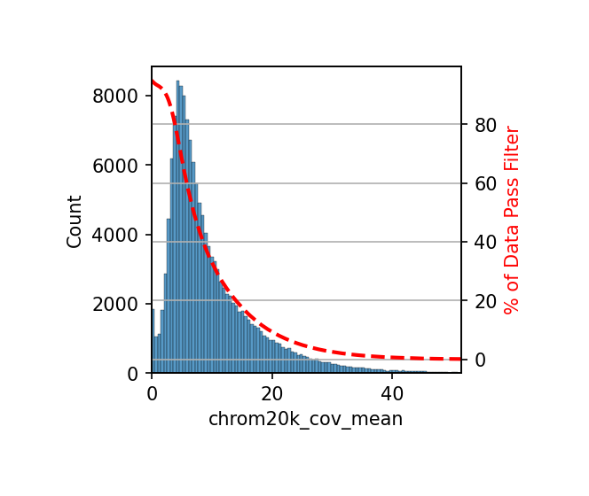
Filter features based on mean coverage to retain high-quality feature regions. This is a crucial step to ensure the quality of DMB analysis.

Importance of Feature Filtering:

• Improve Data Quality: Regions with low coverage may generate noise due to insufficient sequencing depth, affecting the accuracy of differential analysis.
• Reduce False Positives: Filtering out regions with insufficient coverage can lower the false positive rate and improve result reliability.
• Improve Computational Efficiency: Reduce the number of features to be analyzed, speeding up the analysis.

Filtering Workflow:

1. Calculate Mean Coverage: The add_feature_cov_mean() function calculates the average coverage of each 20 kb window across all cells.
2. Set Threshold: Set the min_cov parameter (default is 1) based on data quality, indicating at least 1 cell needs coverage in that region.
3. Filter Features: The filter_feature_by_cov_mean() function removes regions with mean coverage below the threshold.

Parameter Adjustment Suggestions:

• High-Quality Data: Can use min_cov=1 or higher to ensure all retained regions have sufficient coverage.
• Low-Quality Data: If too few features are retained, consider lowering min_cov (e.g., 0.5), but be aware of potential noise introduction.
• Balance: It is recommended to start with the default value; if too few features remain, consider lowering the threshold.

# Calculate feature coverage mean
# Coverage mean reflects average coverage of each 20kb window across all cells
# Used for subsequent feature filtering, filtering out low-quality regions with insufficient coverage

# Set matplotlib plotting parameters
plt.rcParams['figure.dpi'] = 150
plt.rcParams['figure.figsize'] = (3,3)

# Calculate average coverage of each 20kb window across all cells
# Results stored in combined.coords['chrom20k_cov_mean']
combined.add_feature_cov_mean()
print("Feature coverage mean calculation completed")

output

Feature chrom20k mean cov across cells added in MCDS.coords['chrom20k_cov_mean'].
特征覆盖度均值已计算完成

# Filter features based on coverage
# Filter out 20kb windows with average coverage below threshold to improve data quality

min_cov = 1  # Minimum coverage threshold, indicating at least 1 cell has coverage in this region
# If too few features retained, can appropriately lower this value (e.g., 0.5), but may introduce noise

# Filter features: remove windows with average coverage < min_cov
combined.filter_feature_by_cov_mean(min_cov=min_cov)
print(f"Coverage filtering completed, number of retained feature regions: {len(combined.chrom20k)}")

output

Before cov mean filter: 154423 chrom20k
After cov mean filter: 144048 chrom20k 93.3%
覆盖度筛选完成，保留的特征区域数量: 154423

Calculate Methylation Levels and Save MCDS Data

Calculate the methylation level (methylation fraction) for each 20 kb window and save the merged MCDS data for subsequent analysis.

# Calculate methylation fraction
# Methylation fraction = methylated sites / (methylated sites + unmethylated sites)
# Reflects methylation level of each 20kb window (0-1 range)

# normalize_per_cell=True: Normalize per cell to eliminate sequencing depth differences between cells
# clip_norm_value=10: Clip normalized values to within 10 to avoid influence of extreme values
combined.add_mc_frac(normalize_per_cell=True, clip_norm_value=10)

# Keep only methylation fraction data to reduce memory usage
combined = combined[['chrom20k_da_frac']]

# Convert to float32 type to save memory
combined['chrom20k_da_frac'] = combined['chrom20k_da_frac'].astype('float32')

# Save to load directly in subsequent analysis, avoiding recalculation
combined.write_dataset(output_path = 'merge_chrom20k.mcds')
print("MCDS data saved to merge_chrom20k.mcds")

output

Saving chrom20k
Saving chunk 0: 0 - 1000
Saving chunk 1: 1000 - 2000
Saving chunk 2: 2000 - 2226
MCDS数据已保存到 merge_chrom20k.mcds

Differentially Methylated Bins Analysis

Use the one_vs_rest_dmg function to perform differentially methylated bins analysis, identifying specific methylation regions for each cell type relative to other cell types.

设置差异分析参数

min_cov = 1 # 最小覆盖度（已在前面步骤中筛选） obs_dim = 'cell' # 观测维度（细胞） var_dim = 'chrom20k' # 变量维度（20kb窗口） mc_type = 'CGN' # 甲基化类型：CGN表示CG位点的甲基化 top_n = 1000 # 每个细胞类型保留的Top N个差异区间 auroc_cutoff = 0.1 # AUROC阈值，用于过滤区分度较弱的差异区间 adj_p_cutoff = 0.05 # 校正P值阈值（FDR < 0.05视为显著） fc_cutoff = np.inf # Fold Change阈值（设为无穷大表示不限制） max_cluster_cells = 5000 # 每个细胞类型用于分析的最大细胞数（超过会随机采样） max_other_fold = 5 # 其他细胞类型的最大倍数（用于平衡样本量） cpu = 16 # 并行计算的CPU核心数（实际使用中设置为1以避免阻塞）

执行差异甲基化区间分析

one_vs_rest_dmg函数采用"一对多"策略，识别每种细胞类型相对于其他所有细胞类型的特异性甲基化区域

使用Wilcoxon Rank-Sum test进行统计检验，并进行FDR校正

dmb_table = one_vs_rest_dmg(adata_met.obs, # 细胞元数据，包含细胞类型注释 group=anno_col, # 细胞类型注释列名 mcds_paths='merge_chrom20k.mcds', # MCDS数据路径 obs_dim=obs_dim, var_dim=var_dim, mc_type=mc_type, top_n=top_n, adj_p_cutoff=adj_p_cutoff, fc_cutoff=fc_cutoff, auroc_cutoff=auroc_cutoff, max_cluster_cells=max_cluster_cells, max_other_fold=max_other_fold, cpu=1) # 设置为1以避免阻塞

print(f"DMB分析完成，共识别 {len(dmb_table)} 个差异甲基化区间")

保存结果到HDF5格式（高效存储）

dmb_table.to_hdf(f'merge_{var_dim}.OneVsRestDMB.hdf', key='data')

cmd = f'/jp_envs/envs/seeksoulmethyl/bin/python ./run_dmg.py adata_met.h5ad celltype chrom20k merge_chrom20k.mcds'
os.system(cmd)

output

/jp_envs/envs/seeksoulmethyl/lib/python3.10/site-packages/anndata/_core/anndata.py:381: FutureWarning: The dtype argument is deprecated and will be removed in late 2024.
warnings.warn(
/jp_envs/envs/seeksoulmethyl/lib/python3.10/site-packages/anndata/_core/anndata.py:381: FutureWarning: The dtype argument is deprecated and will be removed in late 2024.
warnings.warn(
/jp_envs/envs/seeksoulmethyl/lib/python3.10/site-packages/anndata/_core/anndata.py:381: FutureWarning: The dtype argument is deprecated and will be removed in late 2024.
warnings.warn(
/jp_envs/envs/seeksoulmethyl/lib/python3.10/site-packages/anndata/_core/anndata.py:381: FutureWarning: The dtype argument is deprecated and will be removed in late 2024.
warnings.warn(
/jp_envs/envs/seeksoulmethyl/lib/python3.10/site-packages/anndata/_core/anndata.py:381: FutureWarning: The dtype argument is deprecated and will be removed in late 2024.
warnings.warn(
/jp_envs/envs/seeksoulmethyl/lib/python3.10/site-packages/anndata/_core/anndata.py:381: FutureWarning: The dtype argument is deprecated and will be removed in late 2024.
warnings.warn(
/jp_envs/envs/seeksoulmethyl/lib/python3.10/site-packages/anndata/_core/anndata.py:381: FutureWarning: The dtype argument is deprecated and will be removed in late 2024.
warnings.warn(
/jp_envs/envs/seeksoulmethyl/lib/python3.10/site-packages/anndata/_core/anndata.py:381: FutureWarning: The dtype argument is deprecated and will be removed in late 2024.
warnings.warn(


Calculating cluster B DMGs.
Calculating cluster NK DMGs.
Calculating cluster DC DMGs.
Calculating cluster FCGR3A+ Mono DMGs.
Calculating cluster Memory CD4+ T DMGs.
Calculating cluster CD14+ Mono DMGs.
Calculating cluster Navie CD4+ T DMGs.
Calculating cluster CD8+ T DMGs.
DC Finished.
FCGR3A+ Mono Finished.
B Finished.
CD14+ Mono Finished.
CD8+ T Finished.
NK Finished.
Memory CD4+ T Finished.
Navie CD4+ T Finished.





0

# Read DMB analysis results
dmb_table = pd.read_hdf('merge_chrom20k.OneVsRestDMB.hdf')

# Add genomic coordinate information for bins
bin_info = pd.DataFrame({
    'bin_id': combined["chrom20k"].values, 
    'chrom': combined['chrom20k_chrom'].values, 
    'start': combined['chrom20k_start'].values,
    'end': combined['chrom20k_end'].values}
)

# Merge results
dmb_table = dmb_table.merge(bin_info, left_index = True, right_on = 'bin_id')
# Sort by chrom and bin_id, table index starts from 0
dmb_table = dmb_table.sort_values(['chrom', 'bin_id']).reset_index(drop=True)
print(f"DMB results merged, total {len(dmb_table)} differential methylation bins")
print(dmb_table.head(n=10))

DMB Key Metrics Explanation:

• pvals_adj: P-value after multiple comparison correction (FDR) using Wilcoxon test, reflecting the significance of the bin in the "cluster vs. other cells" comparison.
• fc: Ratio of the average methylation fraction of cells within the cluster to that of cells outside the cluster (in/out fold change). fc < 1 indicates hypomethylation of the cluster relative to other cells.
• AUROC: AUC of the bin in distinguishing "cells within target cluster" vs. "other cells", symmetrized as abs(AUC-0.5)+0.5. Values closer to 1 indicate stronger discrimination.
• cluster: Target cluster.
• bin_id: ID of the bin.
• chrom, start, end: Chromosome number and genomic coordinates where the bin is located.

Differentially Expressed Genes (DEG) Analysis

Differentially Expressed Genes (DEGs) refer to genes with significantly different expression levels in different cell groups. Use the Wilcoxon Rank-Sum test to identify specific marker genes for each cell type.

Significance of DEG Analysis:

• Cell Type Markers: DEGs can serve as specific marker genes for cell type identification and annotation.
• Functional Characteristics: Highly expressed DEGs reflect the main functional characteristics and biological processes of the cell type.
• Multi-omics Integration: Joint analysis of DEGs and DMGs can reveal the regulatory role of epigenetic modifications on gene expression.

Statistical Methods:

• Wilcoxon Rank-Sum test: Non-parametric test method, no assumption on data distribution, suitable for single-cell data characteristics (sparsity, zero-inflation).
• Multiple Comparison Correction: Use Benjamini-Hochberg method for FDR correction to control false discovery rate.
• Effect Size Assessment: Use Log2 Fold Change to assess the magnitude of expression difference, usually filtering with |Log2FC| > 0.25.

Analysis Workflow:

1. Group Comparison: For each cell type, treat it as the target group and all other cell types as the control group.
2. Statistical Test: Perform Wilcoxon test for each gene to calculate significance P-value.
3. Multiple Correction: Perform FDR correction on P-values of all genes to get corrected P-values (pvals_adj).
4. Result Ranking: Rank results based on statistics (scores) or corrected P-values to identify the most significant differential genes.

# Perform differential expression gene analysis using scanpy
# rank_genes_groups function performs 'one-vs-rest' comparison for each cell type
# method='wilcoxon': Use Wilcoxon Rank-Sum test (non-parametric test, suitable for single-cell data)
# groupby=anno_col: Group by cell type
# pts=True: Calculate expression proportion of genes in target and reference groups
sc.tl.rank_genes_groups(adata_rna, method = 'wilcoxon', groupby = anno_col, pts = True)

# Extract differential expression gene results for all cell types
# group=None: Extract results for all cell types
DEG = sc.get.rank_genes_groups_df(adata_rna, group = None)
# Rename column group to cluster, consistent with subsequent analysis
DEG = DEG.rename(columns={'group': 'cluster'})

# Save results to CSV file
DEG.to_csv('DEG.csv', index = False)
print(f"DEG analysis completed, identified total {len(DEG)} differentially expressed genes")
print(DEG.head(n=10))

DEG Key Metrics Explanation:

• cluster: Target cell cluster.
• names: Gene name.
• scores: Z-score statistic; larger absolute values indicate more significant differences.
• logfoldchanges: Log2 Fold Change. Positive values indicate high expression in the target cluster, negative values indicate low expression.
• pvals: Original P-value.
• pvals_adj: P-value after Benjamini-Hochberg correction (FDR). Usually < 0.05 is used as the significance threshold.
• pct_nz_group: Proportion of cells expressing the gene in the target cluster.
• pct_nz_reference: Proportion of cells expressing the gene in other clusters.

Differentially Methylated Genes (DMG) Analysis

Differentially Methylated Genes (DMGs) refer to genes with significantly different methylation levels between different cell types. Analysis is based on methylation levels in the gene region ±2kb (geneslop2k).

Merge Multi-sample MCDS at geneslop2k Methylation Level

# Merge multi-sample MCDS data (geneslop2k level)
# This step is similar to chrom20k merge, but uses gene region ±2kb (geneslop2k) dimension
# geneslop2k dimension contains methylation information for each gene and its upstream/downstream 2kb regions
warnings.filterwarnings('ignore')
mcds_list = []  # Store MCDS object for each sample
cell_number = []  # Record sample belonging for each cell

# Iterate through each sample, read corresponding MCDS data
for i in samples:
    # Extract cell barcode for this sample in methylation data (remove suffix)
    keep_barcodes = [ re.sub('\\-.*','',b) for b in adata_met.obs[adata_met.obs["Sample"] == i].index ] 
    
    # Open MCDS file, use geneslop2k dimension (gene region ±2kb)
    # var_dim='geneslop2k': Specify gene region dimension name
    mcds = MCDS.open(os.path.join('../../','data', sample_path_config[i]['top_dir'], 'methylation', sample_path_config[i]['demo_dir'], i, 'allcools_generate_datasets', f'{i}.mcds'), 
                     obs_dim = 'cell', var_dim = 'geneslop2k', use_obs = keep_barcodes)
    
    # If multiple samples, add sample identifier suffix to each cell barcode
    suffix = samples.index(i)
    if len(samples) > 1:
        mcds = mcds.assign_coords(cell=[ f'{i}-{suffix}' for i in mcds.cell.values ])
    
    mcds_list.append(mcds)
    cell_number += [i]*len(mcds.cell.values)

# Merge MCDS data from all samples
combined_gene = xr.concat(mcds_list, dim="cell")

# Add sample information coordinates
combined_gene = combined_gene.assign_coords(Sample=("cell", cell_number))

# Set dimension attributes of MCDS object
combined_gene.obs_dim = 'cell'
combined_gene.var_dim = 'geneslop2k'

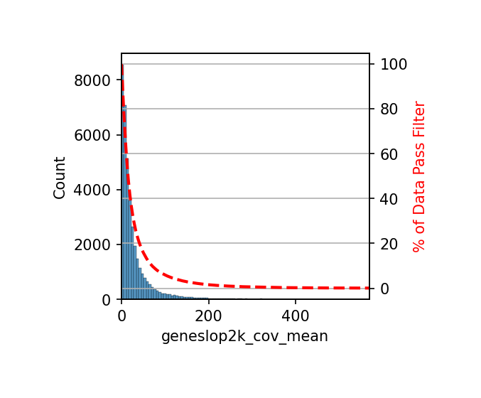
print(f"Merged MCDS data: {len(combined_gene.cell)} cells, {len(combined_gene.geneslop2k)} gene regions")

output

合并后的MCDS数据: 2226 个细胞, 38569 个基因区域

# Calculate feature coverage mean and filter
# Similar to chrom20k analysis, filter gene regions by coverage, retain high-quality regions

plt.rcParams['figure.dpi'] = 150
plt.rcParams['figure.figsize'] = (3,3)

# Calculate average coverage of each gene region across all cells
combined_gene.add_feature_cov_mean()

# Filter features: remove gene regions with average coverage < 1
combined_gene.filter_feature_by_cov_mean(min_cov=1)
print(f"Coverage filtering completed, number of retained gene regions: {len(combined_gene.geneslop2k)}")

output

Feature geneslop2k mean cov across cells added in MCDS.coords['geneslop2k_cov_mean'].
Before cov mean filter: 38569 geneslop2k
After cov mean filter: 37508 geneslop2k 97.2%
覆盖度筛选完成，保留的基因区域数量: 38569

# Calculate true methylation fraction (for subsequent visualization)
combined_gene.add_mc_frac(normalize_per_cell=False, clip_norm_value=None, da_suffix = 'true_frac')
geneslop2k_da_true_frac = combined_gene['geneslop2k_da_true_frac']

# Calculate normalized methylation fraction (for differential analysis)
combined_gene.add_mc_frac(normalize_per_cell=True, clip_norm_value=10)
combined_gene = combined_gene[[f'geneslop2k_da_frac']]
combined_gene[f'geneslop2k_da_frac'] = combined_gene[f'geneslop2k_da_frac'].astype('float32')

# Save merged MCDS data
combined_gene.write_dataset(output_path = 'merge_geneslop2k.mcds')
print("MCDS data saved to merge_geneslop2k.mcds")

output

Saving geneslop2k
Saving chunk 0: 0 - 1000
Saving chunk 1: 1000 - 2000
Saving chunk 2: 2000 - 2226
MCDS数据已保存到 merge_geneslop2k.mcds

Differentially Methylated Genes Analysis

Use the one_vs_rest_dmg function to perform differentially methylated genes (DMG) analysis for each cell type. This function adopts a "one-vs-rest" strategy to identify specific methylated genes for each cell type relative to all other cell types.

Analysis Methods:

• Statistical Test: Wilcoxon Rank-Sum test (Mann-Whitney U test), used to compare differences in methylation levels of gene regions between the target cell type and other cell types.
• Multiple Comparison Correction: Benjamini-Hochberg method (FDR correction), controlling false discovery rate.
• Screening Criteria: Comprehensive screening combining corrected P-value (adj_p_cutoff), Fold Change (fc_cutoff), and AUROC (auroc_cutoff).

设置差异分析参数

min_cov = 1 obs_dim = 'cell' var_dim = 'geneslop2k' mc_type = 'CGN' top_n = 1000 auroc_cutoff = 0.1 adj_p_cutoff = 0.05 fc_cutoff = np.inf max_cluster_cells = 5000 max_other_fold = 5 cpu = 16

执行差异甲基化基因分析

dmg_table = one_vs_rest_dmg(adata_met.obs, group=anno_col, mcds_paths='merge_geneslop2k.mcds', obs_dim='cell', var_dim='geneslop2k', mc_type=mc_type, top_n=top_n, adj_p_cutoff=adj_p_cutoff, fc_cutoff=fc_cutoff, auroc_cutoff=auroc_cutoff, max_cluster_cells=max_cluster_cells, max_other_fold=max_other_fold, cpu=1)

保存结果

dmg_table.to_hdf(f'merge_{anno_col}.OneVsRestDMG.hdf', key='data') print(f"DMG分析完成，共识别 {len(dmg_table)} 个差异甲基化基因")

# If running with external script, can use the following command
cmd = f'/jp_envs/envs/seeksoulmethyl/bin/python ./run_dmg.py adata_met.h5ad celltype geneslop2k merge_geneslop2k.mcds'
os.system(cmd)

output

/jp_envs/envs/seeksoulmethyl/lib/python3.10/site-packages/anndata/_core/anndata.py:381: FutureWarning: The dtype argument is deprecated and will be removed in late 2024.
warnings.warn(
/jp_envs/envs/seeksoulmethyl/lib/python3.10/site-packages/anndata/_core/anndata.py:381: FutureWarning: The dtype argument is deprecated and will be removed in late 2024.
warnings.warn(
/jp_envs/envs/seeksoulmethyl/lib/python3.10/site-packages/anndata/_core/anndata.py:381: FutureWarning: The dtype argument is deprecated and will be removed in late 2024.
warnings.warn(
/jp_envs/envs/seeksoulmethyl/lib/python3.10/site-packages/anndata/_core/anndata.py:381: FutureWarning: The dtype argument is deprecated and will be removed in late 2024.
warnings.warn(
/jp_envs/envs/seeksoulmethyl/lib/python3.10/site-packages/anndata/_core/anndata.py:381: FutureWarning: The dtype argument is deprecated and will be removed in late 2024.
warnings.warn(
/jp_envs/envs/seeksoulmethyl/lib/python3.10/site-packages/anndata/_core/anndata.py:381: FutureWarning: The dtype argument is deprecated and will be removed in late 2024.
warnings.warn(
/jp_envs/envs/seeksoulmethyl/lib/python3.10/site-packages/anndata/_core/anndata.py:381: FutureWarning: The dtype argument is deprecated and will be removed in late 2024.
warnings.warn(
/jp_envs/envs/seeksoulmethyl/lib/python3.10/site-packages/anndata/_core/anndata.py:381: FutureWarning: The dtype argument is deprecated and will be removed in late 2024.
warnings.warn(


Calculating cluster DC DMGs.
Calculating cluster FCGR3A+ Mono DMGs.
Calculating cluster CD14+ Mono DMGs.
Calculating cluster Navie CD4+ T DMGs.
Calculating cluster CD8+ T DMGs.
Calculating cluster NK DMGs.
Calculating cluster B DMGs.
Calculating cluster Memory CD4+ T DMGs.
DC Finished.
B Finished.
CD8+ T Finished.
CD14+ Mono Finished.
FCGR3A+ Mono Finished.
NK Finished.
Memory CD4+ T Finished.
Navie CD4+ T Finished.





0

# Read DMG analysis results
dmg_table = pd.read_hdf('merge_celltype.OneVsRestDMG.hdf', key='data')

# Save as CSV format
dmg_table.reset_index().to_csv('DMG.csv', index = False)
print(f"DMG results saved, total {len(dmg_table)} differentially methylated genes")
dmg_table = dmg_table.reset_index()
dmg_table['names'] = [ re.sub('.*_','',i) for i in dmg_table['names'] ]
print(dmg_table.head())

DMG Key Metrics Explanation:

• names: Gene name.
• pvals_adj: P-value after multiple comparison correction (FDR) using Wilcoxon test, reflecting the significance of the gene in the "cluster vs. other cells" comparison.
• fc: Ratio of the average methylation fraction of cells within the cluster to that of cells outside the cluster (in/out fold change). fc < 1 indicates hypomethylation of the cluster relative to other cells.
• AUROC: AUC of the gene in distinguishing "cells within target cluster" vs. "other cells", symmetrized as abs(AUC-0.5)+0.5. Values closer to 1 indicate stronger discrimination.
• cluster: Target cluster.

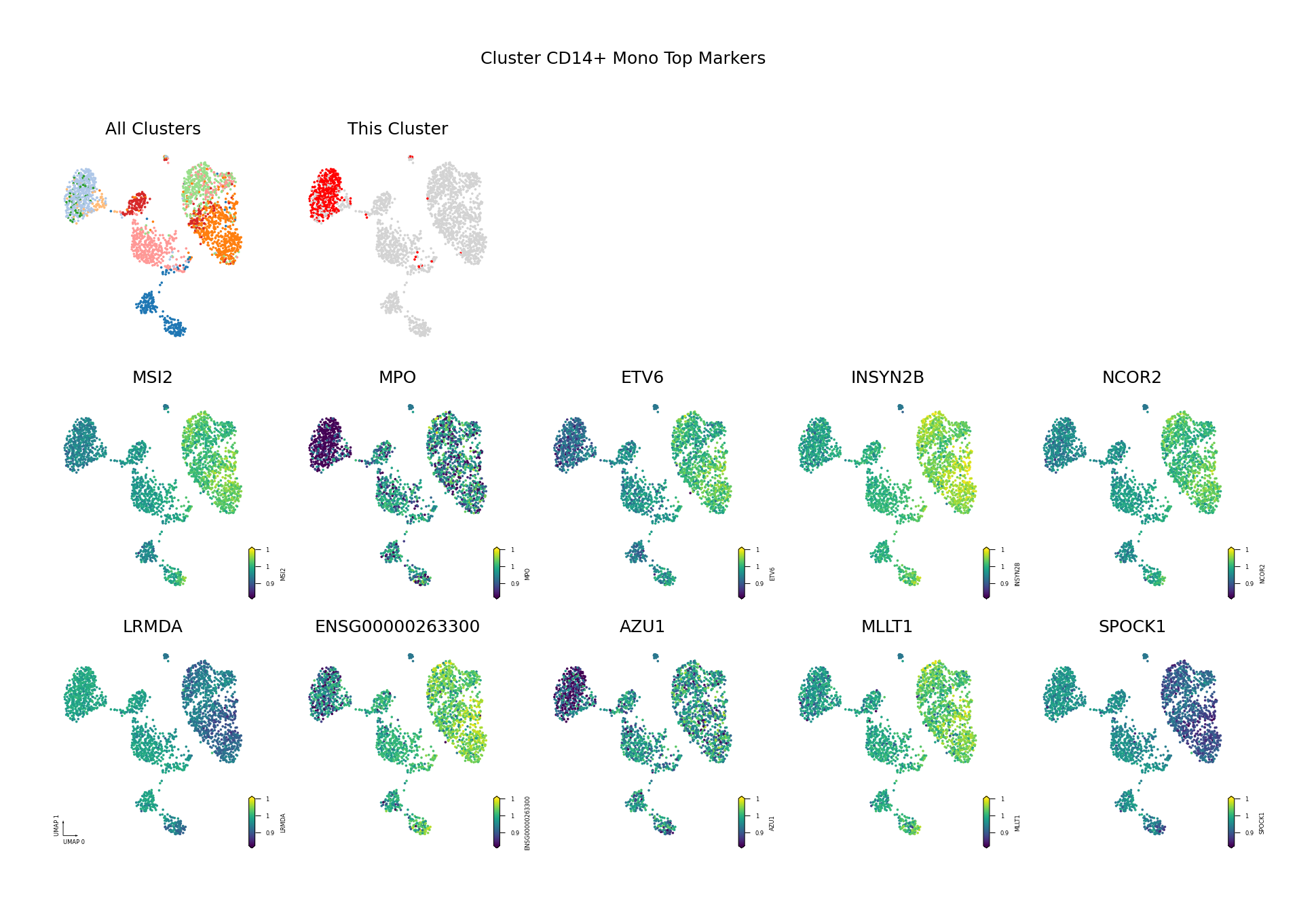
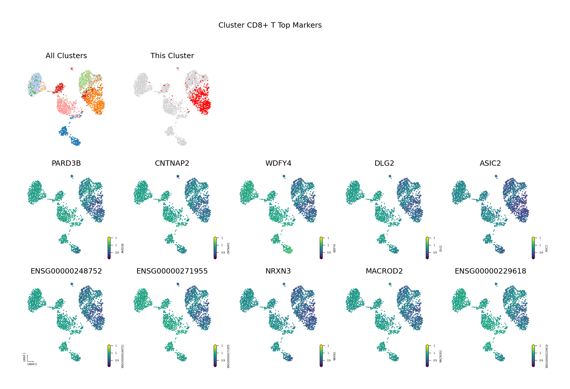
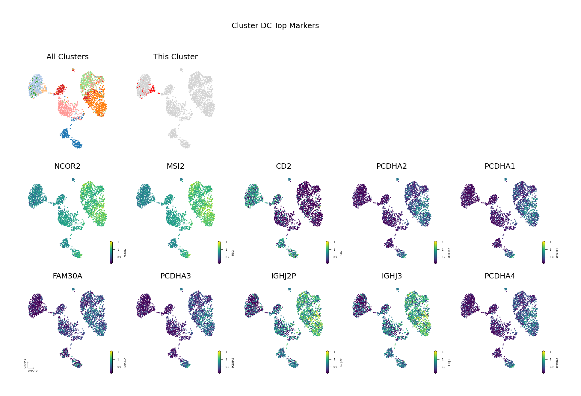
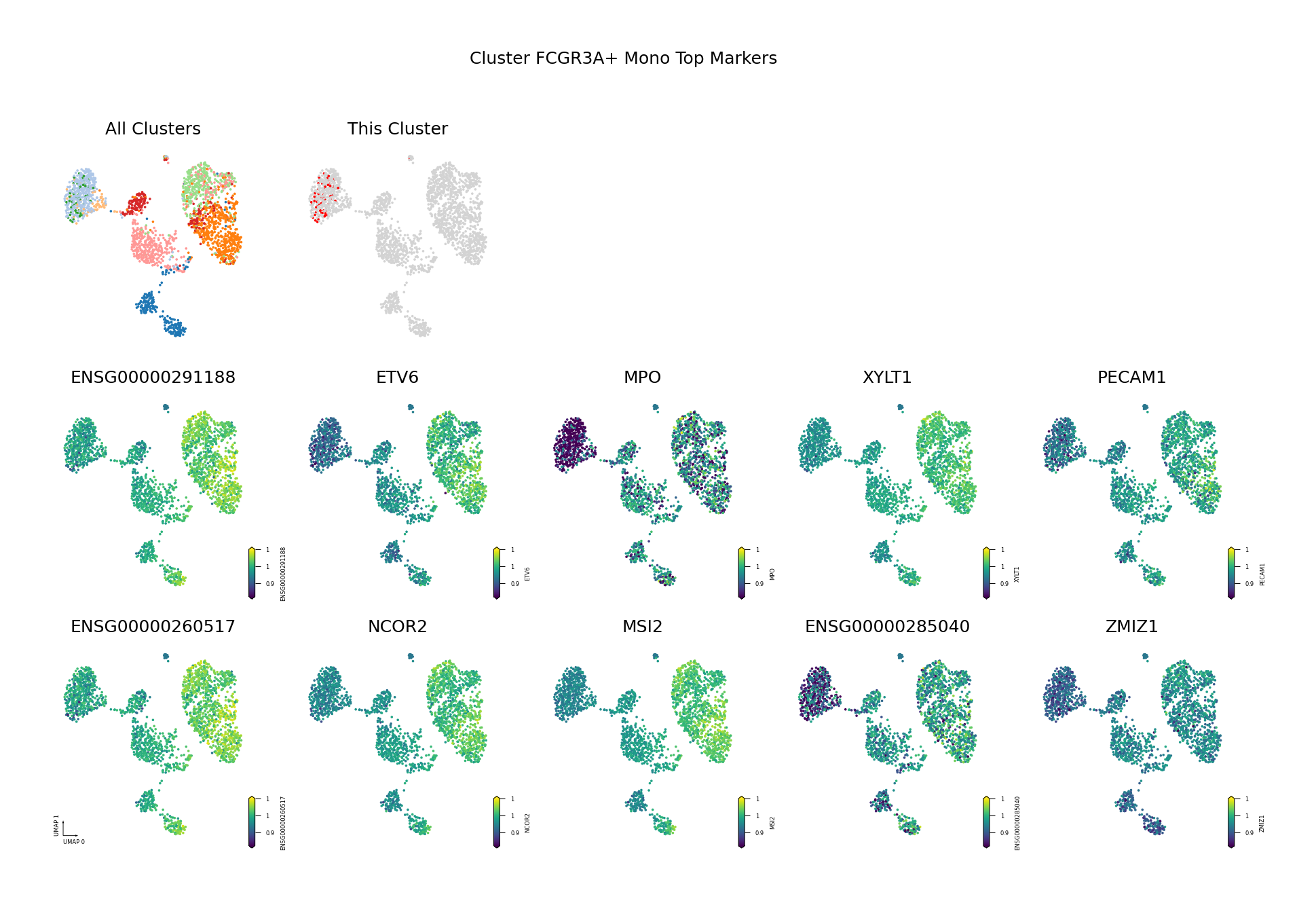
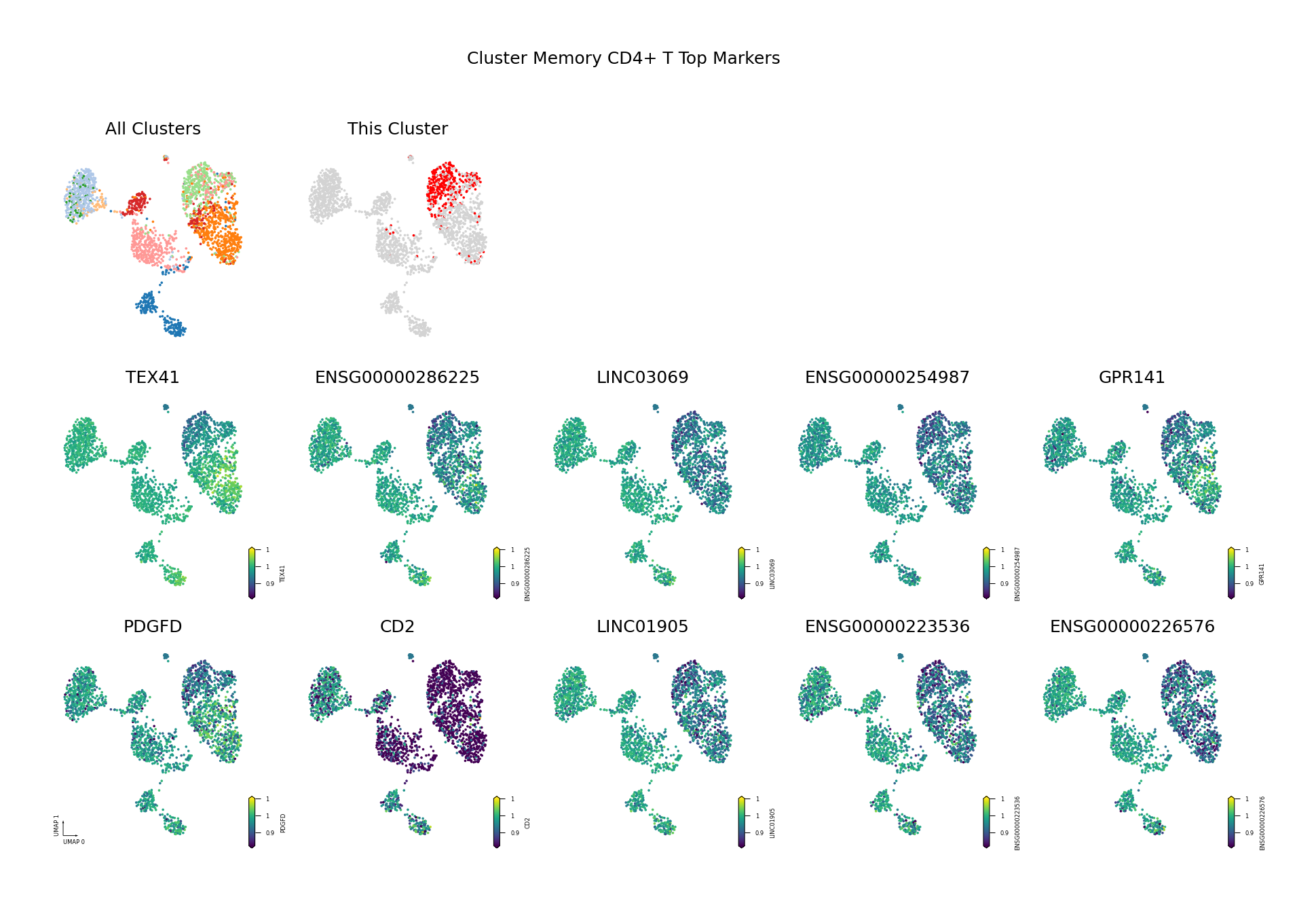
Visualization of Differentially Methylated Genes

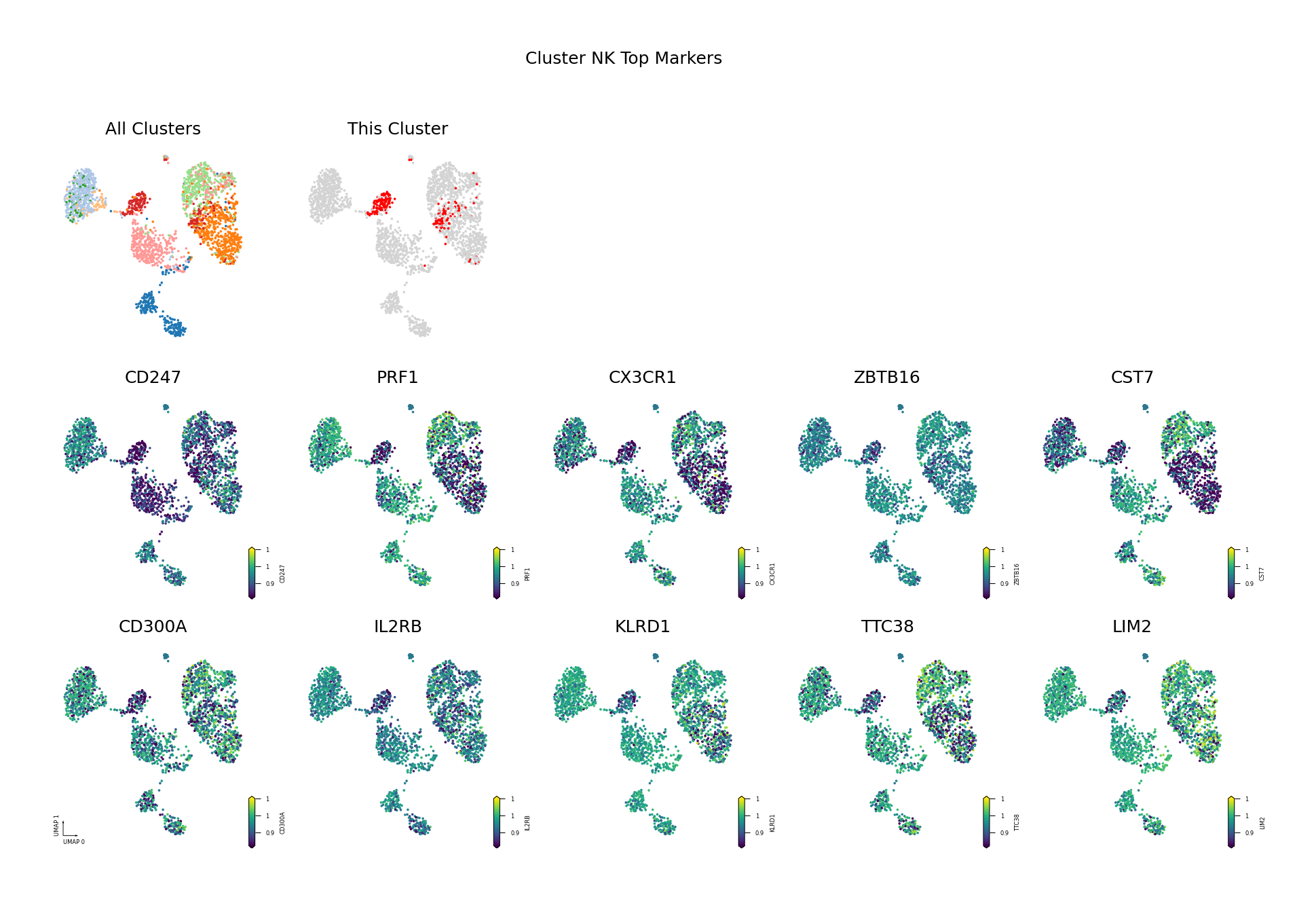
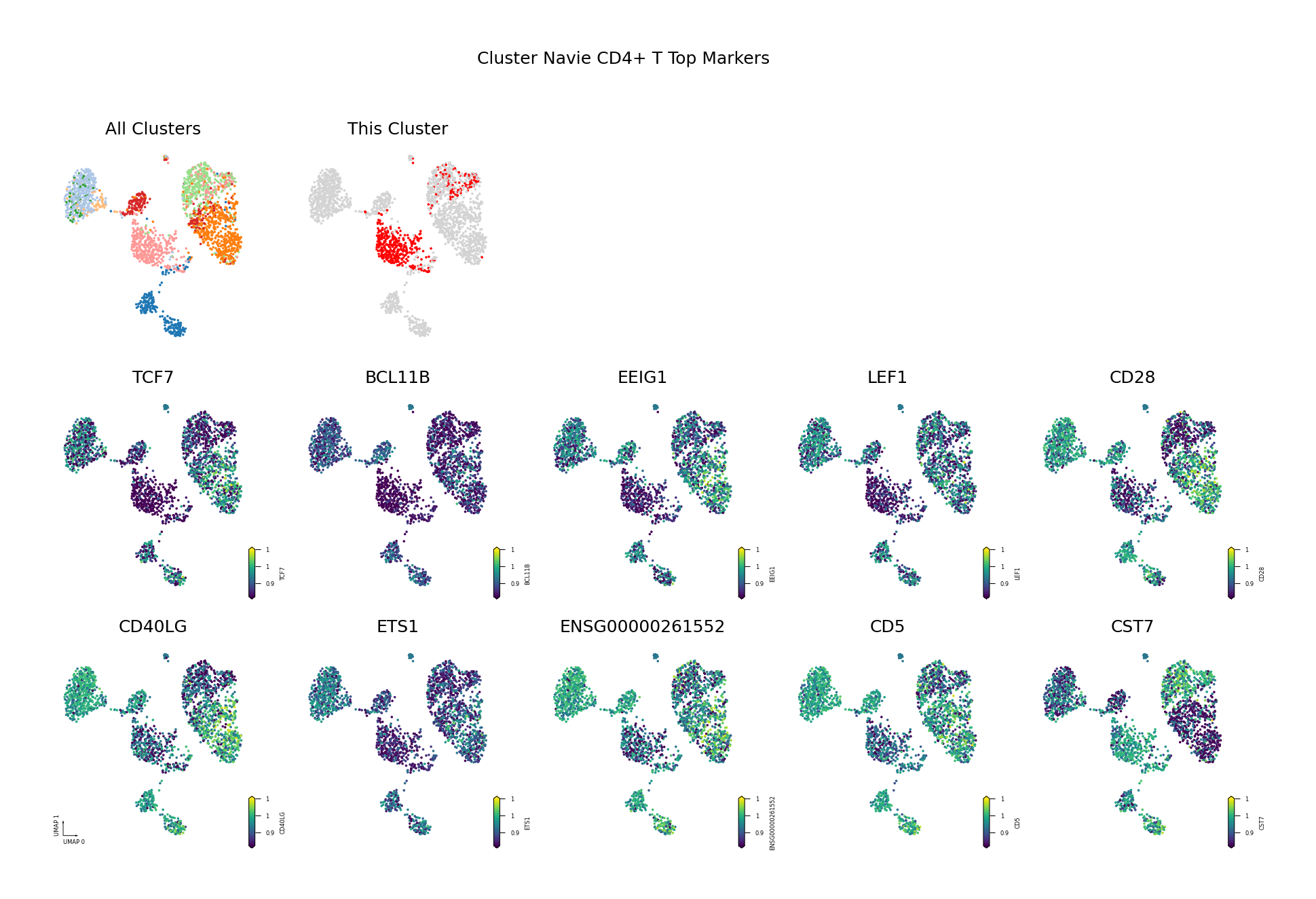
To visually display the identified differentially methylated genes, we project the methylation levels of the filtered Top DMGs (sorted by AUROC, showing only the top 10) onto the UMAP space.

Visualization Purpose:

• Verify Differential Patterns: Verify via UMAP visualization whether the identified DMGs indeed show specific methylation patterns in the target cell type.
• Spatial Distribution: Observe the distribution of DMG methylation levels in UMAP space and whether it aligns with cell type boundaries.
• Discover Patterns: Identify genes with similar methylation patterns that may participate in the same biological processes.

Screening Criteria: AUROC > 0.6 and (Fold Change < 0.9 or > 1.1)

• AUROC > 0.6: Ensure the gene has good discrimination ability to effectively distinguish the target cell type from other cell types.
• Fold Change Threshold: Screen for genes with obvious methylation differences.
  • FC < 0.9: Hypomethylated genes (lower methylation level in target cell type).
  • FC > 1.1: Hypermethylated genes (higher methylation level in target cell type).

Figure Legend: This figure shows the distribution of methylation levels of the Top 10 Differentially Methylated Genes (DMGs) for each cell type in the UMAP reduced dimensional space.

• First Row Left: UMAP plot of all cell types, with different colors representing different cell types, showing overall cell distribution and boundaries.
• First Row Right: UMAP plot of the target cell type, highlighting the target cell type in red and others in gray.
• Subsequent Subplots: Distribution of methylation levels for each Top 10 DMG in UMAP space, one gene per subplot.
• X/Y Axis: UMAP_1 and UMAP_2, representing the two principal dimensions after dimensionality reduction.
• Color: Represents methylation level (fraction); darker (red/yellow) indicates higher, lighter (blue/purple) indicates lower.
• Points: Each point represents a cell, and the position reflects similarity between cells.

def plot_cluster_and_genes(cluster, cell_meta, cluster_col, genes_data,
                           coord_base='umap', ncols=5, axes_size=3, dpi=150, hue_norm=(0.67, 1.5)):
    """Plot UMAP visualization of cell types and Top DMGs"""
    ncols = max(2, ncols)
    nrows = 1 + (genes_data.shape[1] - 1) // ncols + 1

    # figure
    fig = plt.figure(figsize=(ncols * axes_size, nrows * axes_size), dpi=dpi)
    gs = fig.add_gridspec(nrows=nrows, ncols=ncols)

    # cluster axes
    ax = fig.add_subplot(gs[0, 0])
    categorical_scatter(data=cell_meta,
                        ax=ax,
                        coord_base=coord_base,
                        axis_format=None,
                        hue=cluster_col,
                        palette='tab20')
    ax.set_title('All Clusters')
    ax = fig.add_subplot(gs[0, 1])
    categorical_scatter(data=cell_meta,
                        ax=ax,
                        coord_base=coord_base,
                        hue=cell_meta.obs[cluster_col] == cluster,
                        axis_format=None,
                        palette={
                            True: 'red',
                            False: 'lightgray'
                        })
    ax.set_title('This Cluster')

    # gene axes
    for i, (gene, data) in enumerate(genes_data.items()):
        col = i % ncols
        row = i // ncols + 1
        ax = fig.add_subplot(gs[row, col])

        if ax.get_subplotspec().is_first_col() and ax.get_subplotspec().is_last_row():
            axis = 'tiny'
        else:
            axis = None

        continuous_scatter(ax=ax,
                           data=cell_meta,
                           hue=data,
                           axis_format=axis,
                           hue_norm=hue_norm,
                           coord_base=coord_base)
        ax.set_title(f'{data.name}')
    fig.suptitle(f'Cluster {cluster} Top Markers')
    return fig

# Prepare gene annotation information
dmg_table = pd.read_csv("DMG.csv",index_col=0)
clusters = sorted(set(dmg_table['cluster']))
geneslop2k_bed = pd.DataFrame({
    'geneslop2k_id': combined_gene['geneslop2k'].values,
    'geneslop2k_gene_ids': [ re.sub('_.*','',i) for i in combined_gene['geneslop2k'].values ],
    'geneslop2k_name': [ re.sub('.*_','',i) for i in combined_gene['geneslop2k'].values],
    'geneslop2k_chrom': combined_gene['geneslop2k_chrom'].values,
    'geneslop2k_start': combined_gene['geneslop2k_start'].values,
    'geneslop2k_end':combined_gene['geneslop2k_end'].values,
})

gene_name_to_gene_id = {v.geneslop2k_name:v.geneslop2k_id for idx, v in geneslop2k_bed.iterrows()}
geneslop2k_bed = geneslop2k_bed.set_index('geneslop2k_id')

# Filter significant DMGs
dmg_table_plot = dmg_table[(dmg_table.AUROC > 0.6) & ((dmg_table.fc < 0.9) | (dmg_table.fc > 1.1))]

# Downsample to save memory
downsample = 30000
if downsample and (adata_met.n_obs > downsample):
    use_cells = adata_met.obs.sample(downsample, random_state=0).index
    adata_met_subset = adata_met[adata_met.obs_names.isin(use_cells), :].copy()
else:
    use_cells = adata_met.obs_names
    adata_met_subset = adata_met

# Load gene methylation data
gene_frac_da = MCDS.open(f'merge_geneslop2k.mcds',use_obs=use_cells)[f'geneslop2k_da_frac']
gene_frac_da = gene_frac_da.load()

# Plot Top DMGs for each cluster
for cluster in clusters:
    genes = dmg_table_plot[dmg_table_plot['cluster'] == cluster].sort_values('AUROC', ascending=False)[:10]
    if genes.shape[0] < 1:
        continue
    else:
        genes_data = gene_frac_da.sel(geneslop2k=genes.index).to_pandas()
        genes_data.columns = genes_data.columns.map(geneslop2k_bed['geneslop2k_name'])
        fig = plot_cluster_and_genes(cluster=cluster,
                             cell_meta=adata_met,
                             cluster_col=anno_col,
                             genes_data=genes_data,
                             coord_base='umap',
                             ncols=5,
                             axes_size=3,
                             dpi=150)
        # Optional: Save figure
        # fig.savefig(f'figures/{cluster.replace(" ","_")}.TopDMG.pdf',dpi=300,  bbox_inches='tight')
        # fig.savefig(f'figures/{cluster.replace(" ","_")}.TopDMG.png', dpi=300, bbox_inches='tight')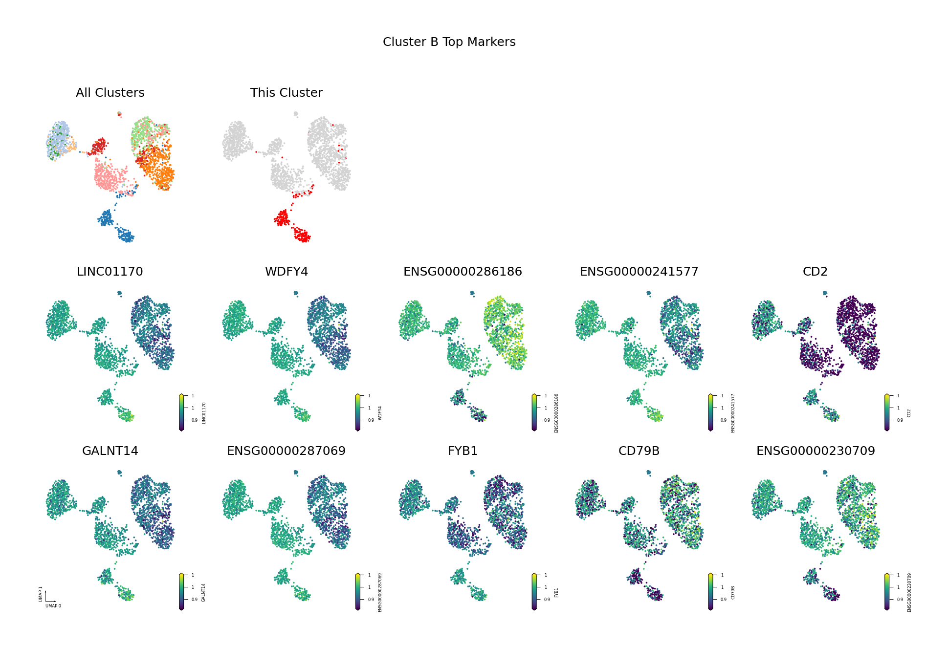

Multi-omics Association Analysis

Integrate transcriptome (RNA) and methylation (Methylation) data to reveal the regulatory relationship between epigenetic modifications and gene expression. Typically, hypermethylation in the gene promoter region inhibits gene expression (negative correlation), but the relationship between gene body methylation and expression may be more complex.

Significance of Multi-omics Association Analysis:

• Reveal Regulatory Mechanisms: Integrating transcriptome and methylation data helps identify the regulatory role of epigenetic modifications on gene expression.
• Discover Key Genes: Genes with both differential expression and differential methylation may be key regulators of cell type differentiation and function.
• Understand Biological Processes: Multi-omics integration helps understand the epigenetic basis of cell type-specific functions.

Association Patterns Between Methylation and Expression:

• Promoter Hypermethylation → Low Expression: Most common negative correlation pattern; hypermethylation in the promoter region usually inhibits gene transcription.
• Promoter Hypomethylation → High Expression: Hypomethylation in the promoter region usually promotes gene transcription.
• Gene Body Methylation: The relationship between gene body methylation and expression is complex and may vary by gene type.
• Enhancer Methylation: Methylation changes in enhancer regions may affect the expression of distant genes.

Analysis Content:

1. Overlap Analysis: Identify genes with both DEG and DMG status; these genes may be key targets of epigenetic regulation.
2. Directionality Analysis: Analyze the association pattern between expression change direction (high/low expression) and methylation change direction (hyper/hypo-methylation).
3. Visualization: Visually display the association of multi-omics data using Venn diagrams and Circos plots.

# Prepare DMG data
dmg_table['met_status'] = ['hypo_met' if i < 1 else 'hyper_met' for i in dmg_table['fc']]
dmg_table['gene_ids'] = [ re.sub('_.*','',i) for i in dmg_table.index ]
dmg_table['gene_names'] = [ re.sub('.*_','',i) for i in dmg_table.index ]

# Prepare DEG data
deg_table = DEG.copy()
deg_table = deg_table.merge(adata_rna.var[['gene_ids']], left_on = 'names', right_index = True, how = 'left')
deg_table['cluster_gene'] = deg_table['cluster'].str.cat(deg_table['gene_ids'],sep = '_')
deg_table = deg_table[(deg_table.pvals_adj < 0.05) & (abs(deg_table.logfoldchanges) > 0.25)]
deg_table['exp_status'] = np.where(deg_table['logfoldchanges'] > 0, 'high_exp', 
                                    np.where(deg_table['logfoldchanges'] < 0, 'low_exp', 'neutral'))

# Merge DEG and DMG data
rename_col = {}
for i in dmg_table.columns:
    rename_col[i] = f'met_{i}'
dmg_table_renamed = dmg_table.rename(columns = rename_col)
dmg_table_renamed['cluster_gene'] = dmg_table_renamed['met_cluster'].str.cat(dmg_table_renamed['met_gene_ids'], sep = '_')

merge_deg_dmg = deg_table.merge(dmg_table_renamed, how = 'outer', left_on = 'cluster_gene', right_on = 'cluster_gene')
conditions = [
    (merge_deg_dmg['logfoldchanges'].notna() & merge_deg_dmg['met_fc'].isna()),
    (merge_deg_dmg['logfoldchanges'].isna() & merge_deg_dmg['met_fc'].notna()),
    (merge_deg_dmg['logfoldchanges'].notna() & merge_deg_dmg['met_fc'].notna()),
    (merge_deg_dmg['logfoldchanges'].isna() & merge_deg_dmg['met_fc'].isna()),
]
choices = ['DEG', 'DMG', 'Both', 'Both']
merge_deg_dmg['status'] = np.select(conditions, choices, default='Both')

# Save genes with both DEG and DMG
merge_deg_dmg[merge_deg_dmg['status'] == 'Both'].to_csv('DEG_DMG.csv', index = False)
print(f"Multi-omics association analysis completed, total {len(merge_deg_dmg[merge_deg_dmg['status'] == 'Both'])} genes with both DEG and DMG")

# Add genomic coordinate information
dmg_table_renamed = dmg_table_renamed.merge(geneslop2k_bed, right_on = 'geneslop2k_gene_ids', left_on = 'met_gene_ids', how = 'left')
deg_table = deg_table.merge(geneslop2k_bed, right_on = 'geneslop2k_gene_ids', left_on = 'gene_ids', how = 'left')

output

多组学关联分析完成，共 360 个同时具有DEG和DMG的基因

Overlap Analysis of Differential Genes and Differentially Methylated Genes (Venn Diagrams)

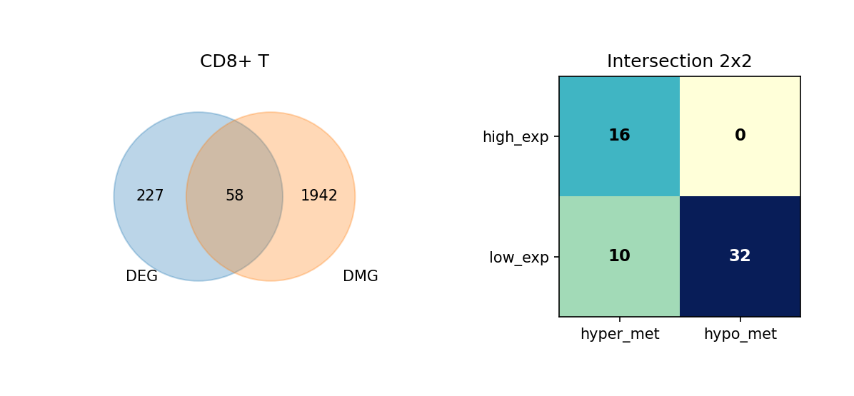
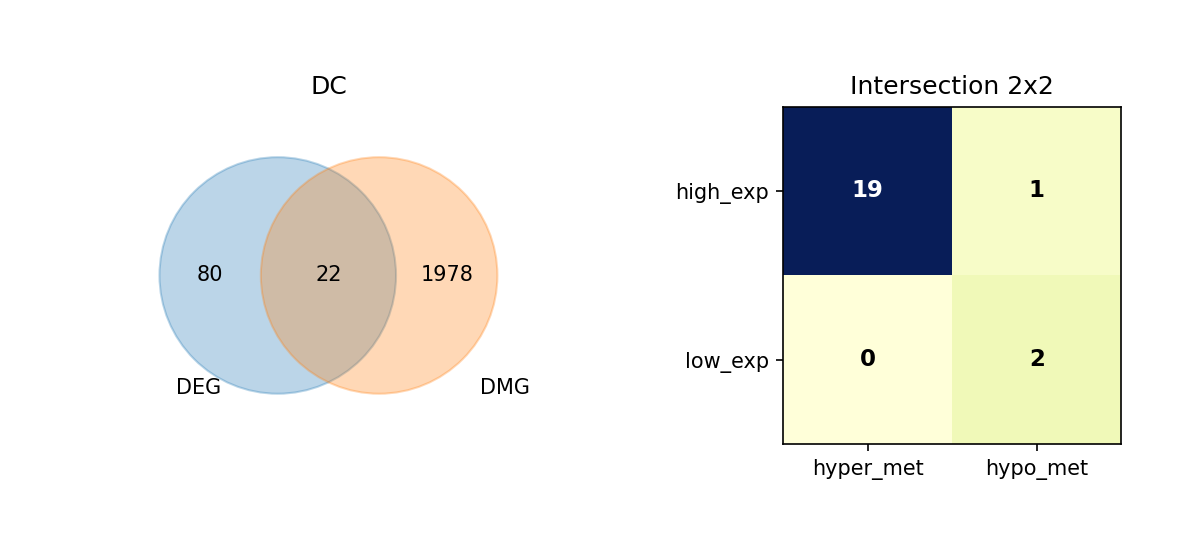
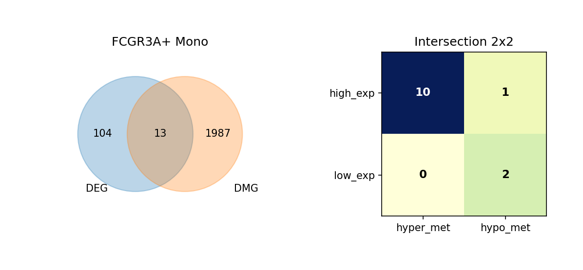
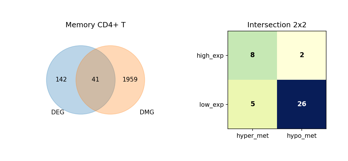
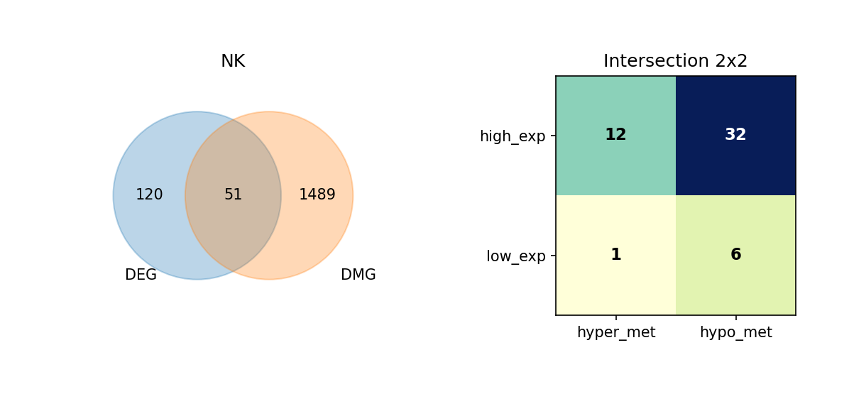
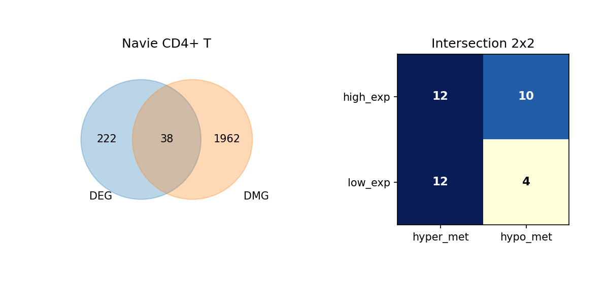
Using Venn diagrams, we display the intersection of DEGs and DMGs in each cell type and further subdivide the expression and methylation change directions of these overlapping genes.

Significance of Overlap Analysis:

• Identify Key Genes: Genes with both differential expression and differential methylation may be key regulators of cell type differentiation and function.
• Epigenetic Regulation: Overlapping genes may be regulated by epigenetic modifications, serving as important clues for understanding epigenetic-transcriptional regulation relationships.
• Functional Association: Overlapping genes may participate in cell type-specific biological processes, worthy of further in-depth study.

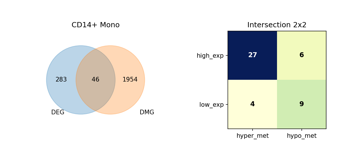
Figure Legend: This figure shows the overlap of DEGs and DMGs in each cell type, as well as the expression and methylation change directions of overlapping genes.

• Left Venn Diagram: Overlap of DEG and DMG; left is DEG only, right is DMG only, middle is the number of overlapping genes.
• Right 2×2 Matrix Heatmap: Overlapping genes subdivided by expression and methylation directions.
  • Rows: Expression direction (high_exp, low_exp).
  • Columns: Methylation direction (hyper_met, hypo_met).
  • Cell Value: Number of genes in that combination; darker color (blue) indicates higher quantity.

HAS_VENN = False
def make_plot_for_cluster(cluster, deg_df, dmg_df, outdir):
    """Plot Venn diagram and 2x2 matrix for each cluster"""
    deg_sub = deg_df[deg_df['cluster'] == cluster].copy()
    dmg_sub = dmg_df[dmg_df['met_cluster'] == cluster].copy()
    deg_set = set(deg_sub['gene_ids'])
    dmg_set = set(dmg_sub['met_gene_ids'])
    inter = deg_set & dmg_set
    deg_only = len(deg_set - inter)
    dmg_only = len(dmg_set - inter)
    inter_count = len(inter)
    
    if 'met_status' not in dmg_sub.columns and 'met_fc' in dmg_sub.columns:
        dmg_sub['met_status'] = np.where(dmg_sub['met_fc'] >= 1, 'hyper_met', 'hypo_met')
    
    inter_df = pd.merge(deg_sub[['gene_ids','exp_status']], 
                        dmg_sub[['met_gene_ids','met_status']], 
                        left_on='gene_ids', right_on='met_gene_ids', how='inner')
    inter_df = inter_df[inter_df['exp_status'] != 'neutral']
    
    def count(exp, met):
        return int(((inter_df['exp_status'] == exp) & (inter_df['met_status'] == met)).sum())
    
    counts = {
      ('high_exp','hyper_met'): count('high_exp','hyper_met'),
      ('high_exp','hypo_met'): count('high_exp','hypo_met'),
      ('low_exp','hyper_met'): count('low_exp','hyper_met'),
      ('low_exp','hypo_met'): count('low_exp','hypo_met')
    }
    
    fig, axes = plt.subplots(1, 2, figsize=(8, 3), dpi = 150)
    ax = axes[0]
    
    if HAS_VENN:
        from matplotlib_venn import venn2
        v = venn2(subsets=(deg_only, dmg_only, inter_count), set_labels=('DEG', 'DMG'), ax=ax)
    else:
        from matplotlib.patches import Circle
        ax.set_aspect('equal')
        c1 = Circle((0.6, 0.5), 0.35, color='C0', alpha=0.3)
        c2 = Circle((0.9, 0.5), 0.35, color='C1', alpha=0.3)
        ax.add_patch(c1)
        ax.add_patch(c2)
        ax.text(0.4, 0.5, str(deg_only), ha='center', va='center')
        ax.text(0.75, 0.5, str(inter_count), ha='center', va='center')
        ax.text(1.1, 0.5, str(dmg_only), ha='center', va='center')
        ax.set_xlim(0, 1.5)
        ax.set_ylim(0, 1)
        ax.axis('off')
        ax.text(0.3, 0.15, 'DEG')
        ax.text(1.2, 0.15, 'DMG')
    
    ax.set_title(cluster)
    ax2 = axes[1]
    matrix = np.array([[counts[('high_exp','hyper_met')], counts[('high_exp','hypo_met')]],
                       [counts[('low_exp','hyper_met')], counts[('low_exp','hypo_met')]]])
    im = ax2.imshow(matrix, cmap='YlGnBu')
    thr = matrix.max() / 2 if matrix.max() > 0 else 0
    for i in range(2):
        for j in range(2):
            color = 'white' if matrix[i, j] > thr else 'black'
            ax2.text(j, i, matrix[i, j], ha='center', va='center', color=color, fontsize=11, fontweight='bold')
    ax2.set_xticks([0, 1])
    ax2.set_xticklabels(['hyper_met', 'hypo_met'])
    ax2.set_yticks([0, 1])
    ax2.set_yticklabels(['high_exp', 'low_exp'])
    ax2.set_title('Intersection 2x2')
    fig.tight_layout()
    plt.show()
    return {'deg_only': deg_only, 'dmg_only': dmg_only, 'inter': inter_count, 'counts': counts}

# Plot Venn diagram for each cluster
results = {}
for cluster in clusters:
    results[cluster] = make_plot_for_cluster(cluster, deg_table, dmg_table_renamed, "./")

# Generate summary table
summary_df = pd.DataFrame.from_dict({k: v['counts'] for k, v in results.items()}, orient='index')
summary_df.columns = [ (f"{c[0]}|{c[1]}" if isinstance(c, tuple) else str(c)) for c in summary_df.columns ]
summary_df.to_csv('summary_counts.csv')
print("Venn diagram analysis completed, results saved to summary_counts.csv")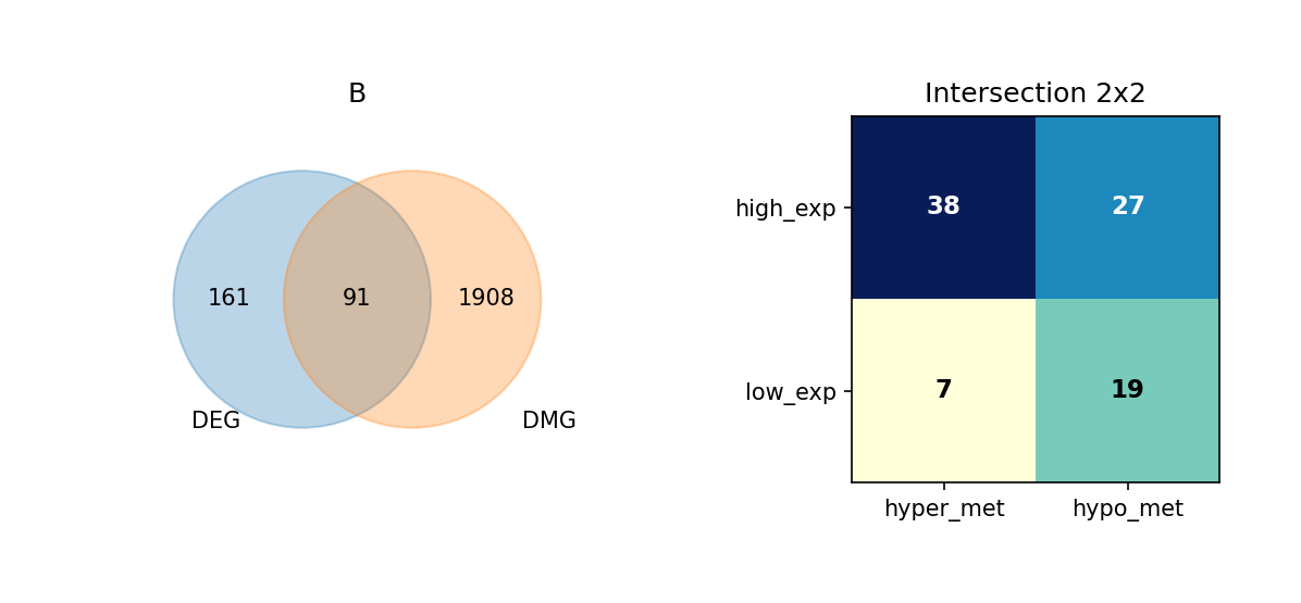

Venn图分析完成，结果已保存到 summary_counts.csv

Figure Legend: This figure summarizes the expression/methylation directions of DEG and DMG overlapping genes across all cell types.

• X-axis: Combinations of expression and methylation directions (e.g., high_exp|hyper_met, low_exp|hypo_met, etc.).
• Y-axis: Cell type (celltype).
• Heatmap Color: Represents gene count; darker (blue) is more, lighter (yellow/white) is less.
• Cell Value: Number of genes for that cell type in that direction combination; color bar on the right shows the value range.

# Plot summary heatmap
cols_order = ['high_exp|hyper_met','high_exp|hypo_met','low_exp|hyper_met','low_exp|hypo_met']
plot_df = summary_df.reindex(columns=cols_order)
fig, ax = plt.subplots(figsize=(4,4))
im = ax.imshow(plot_df.values, cmap='YlGnBu', aspect='auto')
ax.set_xticks(range(len(cols_order)))
ax.set_xticklabels(cols_order, rotation=45, ha='right')
ax.set_yticks(range(len(plot_df)))
ax.set_yticklabels(plot_df.index)
thr = plot_df.values.max() / 2 if plot_df.values.max() > 0 else 0
for i in range(plot_df.shape[0]):
    for j in range(plot_df.shape[1]):
        val = int(plot_df.values[i,j])
        color = 'white' if val > thr else 'black'
        ax.text(j, i, val, ha='center', va='center', color=color, fontsize=10, fontweight='bold')
fig.colorbar(im, ax=ax, fraction=0.046, pad=0.04)
fig.tight_layout()
plt.show()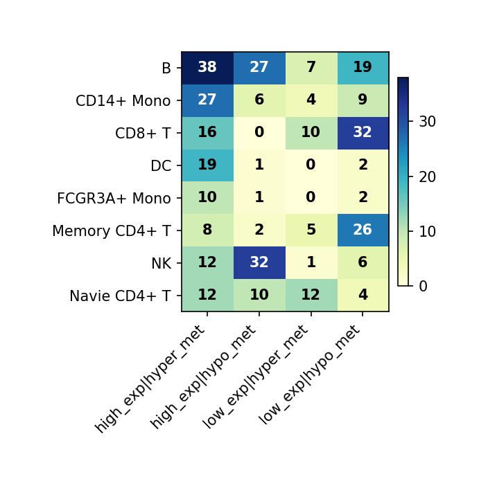

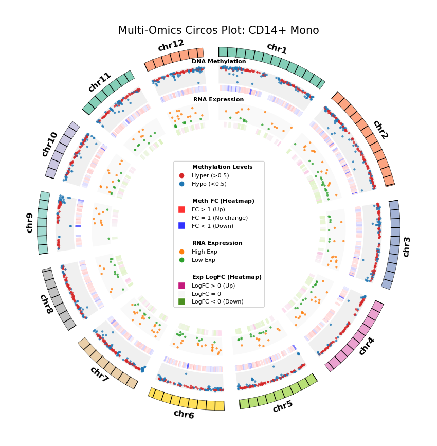
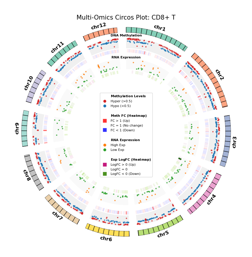
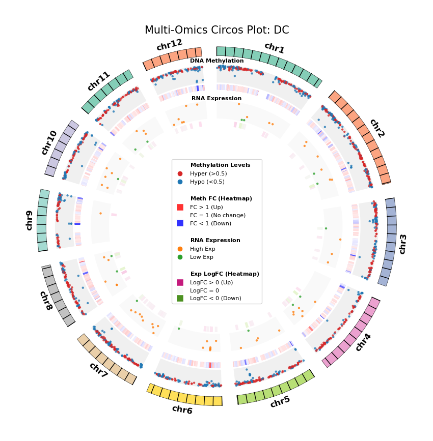
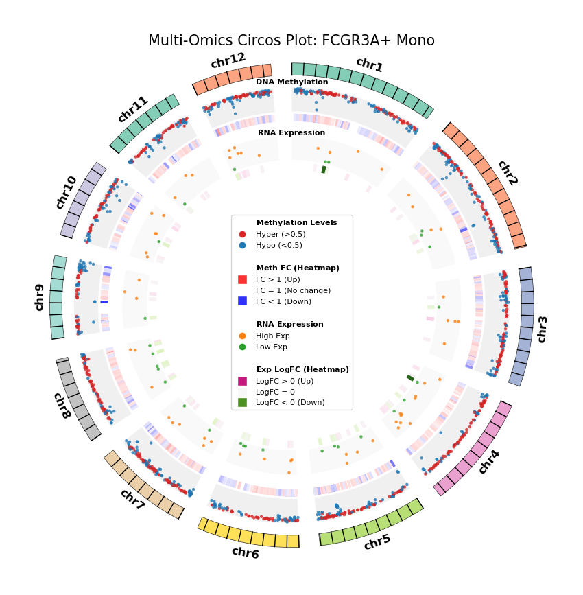
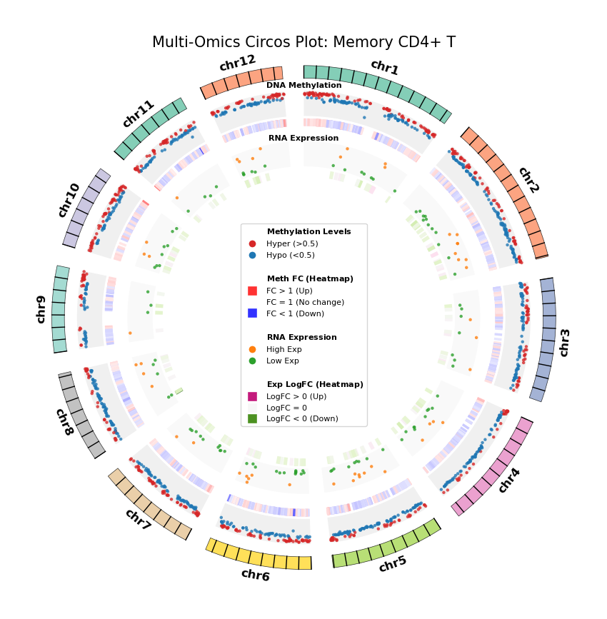
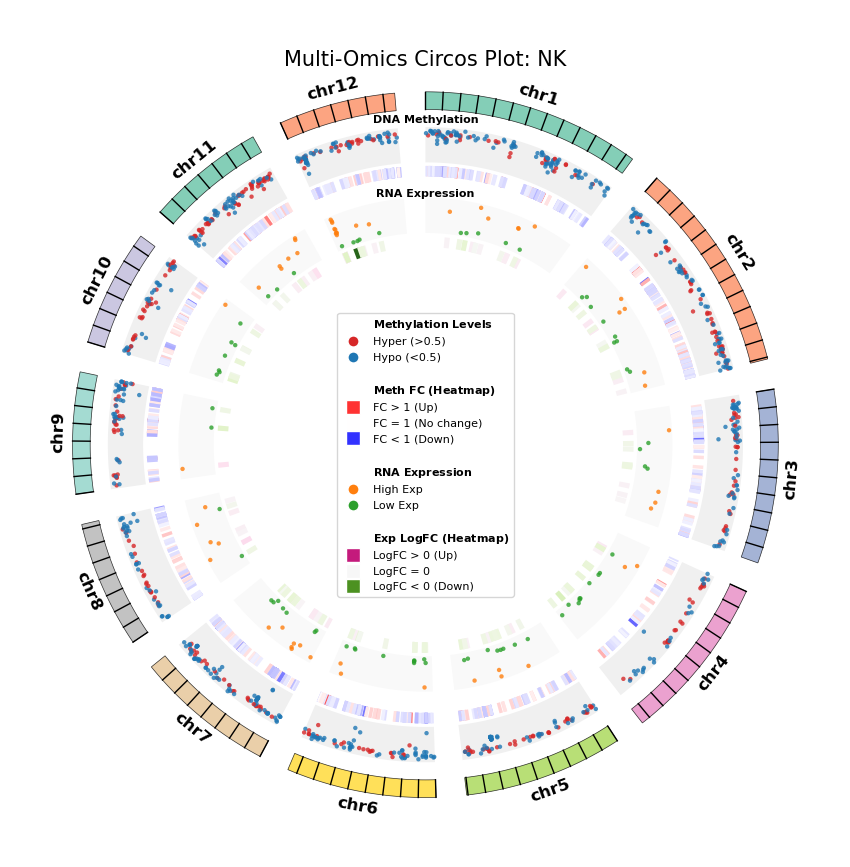
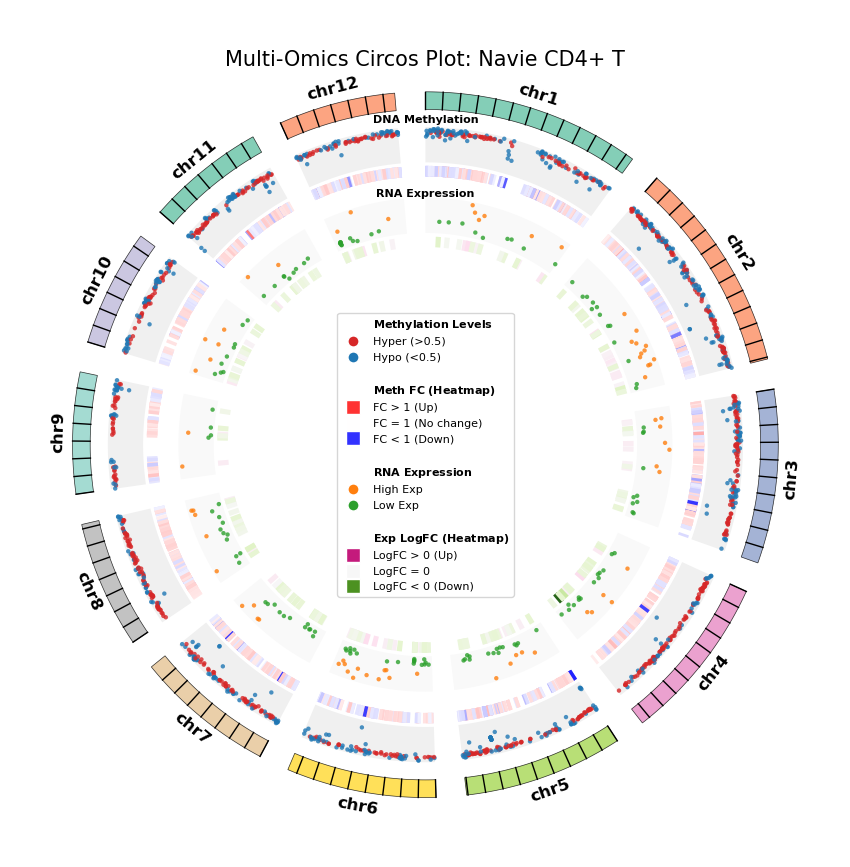
Circos Plot Display of Differential Genes and Differentially Methylated Genes

We use Circos plots to display the distribution and correspondence of DEGs and DMGs on a genome-wide scale. This circular visualization simultaneously shows chromosomal positions, methylation changes, and gene expression changes, intuitively revealing the spatial association of multi-omics data.

Advantages of Circos Plot:

• Genome-wide Perspective: Can display data from all chromosomes simultaneously, providing a global view.
• Spatial Association: Can visually see the positional relationship of DEGs and DMGs on the genome, identifying co-localization patterns.
• Multi-dimensional Information: Display position, methylation level, and expression level in one plot, facilitating discovery of associations.

Figure Legend: Genome-wide Joint Distribution of DNA Methylation Differential Genes (DMG) and RNA Differentially Expressed Genes (DEG) (Circos Plot)

This figure shows the correspondence and spatial distribution characteristics of DNA methylation and gene expression differences on a genome-wide scale (selecting representative chromosomes).

• Outer Circle (Chromosome): Displays chromosome numbers and coordinate scales, with different colors distinguishing each chromosome.
• Middle Layer (DNA Methylation):
  • Scatter Plot: Displays average methylation level (0–1) of DMGs. Red represents hypermethylation (Hyper), blue represents hypomethylation (Hypo).
  • Heatmap Ring: Displays Fold Change of DMGs. Red bands indicate upregulated methylation levels (FC > 1), blue bands indicate downregulated (FC < 1), color intensity reflects the magnitude of difference.
• Inner Layer (RNA Expression):
  • Scatter Plot: Displays average gene expression level of DEGs. Orange represents high expression (High Exp), green represents low expression (Low Exp).
  • Heatmap Ring: Displays Log2 Fold Change of DEGs. Red/pink bands indicate upregulated expression (Log2FC > 0), green bands indicate downregulated (Log2FC < 0), color intensity reflects the magnitude of difference.

# ==========================================
# Prepare data for Circos plot
# ==========================================
# This step prepares data for Circos plot, including:
# 1. Calculate average methylation level of DMG genes in each cell type
# 2. Calculate average expression level of DEG genes in each cell type
# 3. Merge methylation and expression data, add genomic coordinate information

warnings.filterwarnings('ignore')

# ==========================================
# Part 1: Prepare methylation data (DMG)
# ==========================================

# Filter methylation data, keep only cells present in combined_gene
# Ensure methylation data is consistent with gene region data
adata_met = adata_met[adata_met.obs.index.isin(combined_gene.cell.values)]

# Add cell type annotation coordinates to geneslop2k_da_true_frac
# geneslop2k_da_true_frac is previously calculated true methylation fraction (unnormalized)
geneslop2k_da_true_frac.coords["celltype"] = ('cell', adata_met.obs["celltype"])

# Construct geneslop2k_ids: connect gene ID and gene name with underscore
# Format: gene_id_gene_name (e.g., ENSG00000128731_HERC2)
dmg_table_renamed['geneslop2k_ids'] = dmg_table_renamed['met_gene_ids'].str.cat(dmg_table_renamed['met_gene_names'], sep = '_')

# Calculate average methylation level of each DMG gene in each cell type
# groupby("celltype").mean(dim='cell'): Group by cell type, calculate average methylation level of each gene
# sel(geneslop2k=...): Select only genes in DMG table
geneslop2k_da_true_frac = geneslop2k_da_true_frac.groupby("celltype").mean(dim='cell').sel(geneslop2k = list(set(dmg_table_renamed['geneslop2k_ids'])))

# Convert xarray data to DataFrame for easier merging
df = geneslop2k_da_true_frac.compute().to_dataframe().reset_index()

# Merge average methylation level into DMG table
# Add average methylation level of each DMG gene in each cell type (geneslop2k_da_true_frac column)
dmg_table2 = dmg_table_renamed.merge(df[["celltype",'geneslop2k', 'geneslop2k_da_true_frac']], left_on=['met_cluster', 'geneslop2k_ids'], right_on = ["celltype", 'geneslop2k'], how = 'left')

# ==========================================
# Part 2: Prepare expression data (DEG)
# ==========================================

# Add geneslop2k_ids to transcriptome data for matching with methylation data
adata_rna.var['geneslop2k_ids'] = adata_rna.var['gene_ids'].str.cat(adata_rna.var.index, sep = '_')

# Get all cell types
cell_types = adata_rna.obs["celltype"].unique()

# Create DataFrame to store average expression of each gene in each cell type
# Rows: cell types, Columns: gene IDs
mean_expression = pd.DataFrame(index=cell_types, columns=adata_rna.var['gene_ids'])

# Calculate average expression of each gene in each cell type
for ct in cell_types:
    # Extract all cells of this cell type
    subset = adata_rna[adata_rna.obs["celltype"] == ct].X
    
    # Handle both sparse and dense matrix cases
    if sparse.issparse(subset):
        # Sparse matrix: use .A1 to convert result to 1D array
        mean_val = subset.mean(axis=0).A1
    else:
        # Dense matrix: calculate mean directly
        mean_val = subset.mean(axis=0)
        
    # Store in DataFrame
    mean_expression.loc[ct] = mean_val

# Convert wide format to long format for easier merging
# melt operation: convert rows (cell types) and columns (genes) to rows, each row containing a cell type-gene pair average expression
mean_expression = mean_expression.reset_index().melt(
    id_vars='index',  # Retain cell type column (index)
    var_name='gene_ids',  # Gene ID column name
    value_name='mean_exp')  # Average expression column name

# Merge average expression into DEG table
# Add average expression of each DEG gene in each cell type (mean_exp column)
deg_table2 = deg_table.merge(mean_expression, left_on = ['cluster', 'geneslop2k_gene_ids'], right_on = ['index', 'gene_ids'], how = 'left').drop(['gene_ids_y','index'], axis = 1).rename(columns = {'gene_ids_x':'gene_ids'})

for target_cell_type in clusters:
    # Filter data
    plot_meth = dmg_table2[dmg_table2['met_cluster'] == target_cell_type].copy()
    plot_exp = deg_table2[deg_table2['cluster'] == target_cell_type].copy()

    chrom_sizes = pd.read_table(os.path.join('../../','data', sample_path_config[samples[0]]['top_dir'], 'methylation', sample_path_config[samples[0]]['demo_dir'], samples[0], 'allcools_generate_datasets', f'{samples[0]}.mcds', 'chrom_sizes.txt'), header = None, sep = '\t')

    # chrom_sizes has two columns (chromosome name, length), build sectors by row, and convert length to int for Circos
    def natural_sort_key(chrom_name):
        # Remove 'chr' prefix (if any) and try to convert to number
        # e.g. "chr1" -> 1, "chr10" -> 10
        # "chrX" -> 23, "chrY" -> 24 (Assign a large number to non-numeric chromosomes to place them at the end)
        
        import re
        
        # Extract numeric part from name
        match = re.search(r'(\d+)', chrom_name)
        if match:
            return int(match.group(1))
        
        # If no number (e.g., X, Y, M), manually specify order
        special_chroms = {'X': 100, 'Y': 101, 'M': 102, 'MT': 102, 
                          'chrX': 100, 'chrY': 101, 'chrM': 102}
        return special_chroms.get(chrom_name, 999) # Unknown ones placed at the end
    
    # 2. Read and sort
    sectors_all = {str(row[0]): int(row[1]) for _, row in chrom_sizes.iterrows()} 
    sorted_keys = sorted(sectors_all.keys(), key=natural_sort_key)

    top_n = 12
    sectors = {k: sectors_all[k] for k in sorted_keys[:top_n]}
    circos = Circos(sectors, space=5)
    # ==========================================
    # Prepare Color Maps
    # ==========================================

    # 1. Methylation Fold Change Color Map (Center = 1)
    # 0 (low) -> 1 (white/gray) -> >1 (high)
    min_meth = plot_meth['met_fc'].min()
    max_meth = plot_meth['met_fc'].max()
    
    delta_meth = max(abs(1 - min_meth), abs(max_meth - 1))
    
    # Shrink range slightly (e.g., *0.9) to saturate extreme colors, not waiting for max value to turn red
    limit_meth = delta_meth * 0.9  
    
    norm_meth_fc = mcolors.TwoSlopeNorm(
        vmin=1 - limit_meth, 
        vcenter=1, 
        vmax=1 + limit_meth
    )
    cmap_meth_fc = plt.get_cmap('bwr') # Blue-White-Red
    
    chr_cmap = mcolors.ListedColormap(my_palette)
    sector_colors = {name: chr_cmap(i % 10) for i, name in enumerate(sectors.keys())}
        
    min_exp = plot_exp['logfoldchanges'].min()
    max_exp = plot_exp['logfoldchanges'].max()
    
    # LogFC center is 0
    # Take max absolute value to ensure 0 is white
    limit_exp = max(abs(min_exp), abs(max_exp)) * 0.9 # Also *0.9 to enhance saturation
    
    norm_exp_fc = mcolors.TwoSlopeNorm(
        vmin=-limit_exp, 
        vcenter=0, 
        vmax=limit_exp
    )
    cmap_exp_fc = plt.get_cmap('PiYG_r') # Purple-Green
    # ==========================================
    # 4. Plot Tracks
    # ==========================================
    
    # --- Track 1: Chromosome Name and Ticks ---
    for sector in circos.sectors:
        # 1. Chromosome Name (Bold, slightly moved outward)
        # sector.text(sector.name, r=102, size=12, weight='bold', color=sector_colors[sector.name])
        sector.text(sector.name, r=102, size=12, weight='bold', color="black")

        # 2. Chromosome Band (Use our assigned colors)
        track = sector.add_track((95, 100))
        track.axis(fc=sector_colors[sector.name], alpha=0.8) # 80% opacity, good texture
        
        # 3. Add Ticks (One large tick every 20Mb, with numbers)
        # interval unit is bp, set to 20,000,000 (20Mb) here
        # label_size controls number size, label_orientation adjusts direction
        interval = 20 * 10**6
        limit = int(sector.end - sector.start)
        for pos in range(0, limit, int(interval)):
            # [0, 0.3] means draw line at inner 30% of band width (0 is inner edge, 1 is outer edge)
            track.line([pos, pos], [0, 0.3], color='black', lw=1)
    # ==========================================
    # region A: DNA Methylation Data Area
    # ==========================================
    # Plan:
    # r=90-95: Scatter Plot (Level)
    # r=86-89: Heatmap Band (Fold Change)
    
    for sector in circos.sectors:
        # Get data
        sub_meth = plot_meth[plot_meth['geneslop2k_chrom'] == sector.name]
        
        # --- Track A1: Methylation Level Scatter Plot ---
        track_scatter = sector.add_track((80, 90))
        track_scatter.axis(fc='#f0f0f0', ec='none') 
        
        # Add region label (only add once in the first sector, or find a fixed angle to add)
        if sector.name == circos.sectors[0].name:
            circos.text('DNA Methylation', r=92, size=8, color='black', weight='bold')
    
        if not sub_meth.empty:
            x = sub_meth['geneslop2k_start'].values
            y = sub_meth['geneslop2k_da_true_frac'].values
            status = sub_meth['met_met_status'].values
            colors = np.where(status == 'hyper_met', '#d62728', '#1f77b4')
            track_scatter.scatter(x, y, color=colors, s=10, alpha=0.8, vmin=0, vmax=1)
    
        # --- Track A2: Methylation FC Heatmap Band ---
        track_heatmap = sector.add_track((76, 79))
        # track_heatmap.axis(fc="none", ec="none") # Heatmap background transparent
        
        if not sub_meth.empty:
            # Iterate to draw rectangles (simulate heatmap)
            # width set to 2000 (geneslop2k) or slightly wider for visibility
            for _, row in sub_meth.iterrows():
                
                # Draw rectangle: rect(start, end, ...)
                center = (row['geneslop2k_start'] + row['geneslop2k_end']) / 2
                width = 5000000 # 1Mb
                
                new_start = center - (width / 2)
                new_end = center + (width / 2)
                
                # 2. Critical Fix: Prevent Out of Bounds (Clip)
                # Must be limited within [sector.start, sector.end]
                new_start = max(new_start, sector.start)
                new_end = min(new_end, sector.end)
                
                # 3. If start >= end after clipping, skip drawing 
                if new_start >= new_end:
                 continue
                
                val = row['met_fc'] 
                color = cmap_meth_fc(norm_meth_fc(val)) 
                
                track_heatmap.rect(new_start, new_end, color=color, lw=0) 
    
    # ==========================================
    # region B: RNA Expression Data Area
    # ==========================================
    # Plan:
    # r=70-75: Scatter Plot (Level)
    # r=66-69: Heatmap Band (LogFC)
    
    for sector in circos.sectors:
        sub_exp = plot_exp[plot_exp['geneslop2k_chrom'] == sector.name]
    
        # --- Track B1: Expression Level Scatter Plot ---
        track_scatter = sector.add_track((60, 70))
        track_scatter.axis(fc='#f9f9f9', ec='none')
    
        # Add region label
        if sector.name == circos.sectors[0].name:
            circos.text('RNA Expression', r=71, size=8, color='black', weight='bold')

        if not sub_exp.empty:
            x = sub_exp['geneslop2k_start'].values
            y = sub_exp['mean_exp'].values
            status = sub_exp['exp_status'].values
            colors = np.where(status == 'high_exp', '#ff7f0e', '#2ca02c')
    
            # Solution 1: Manually set appropriate vmin and vmax
            y_min, y_max = y.min(), y.max()
            # Add some margin to ensure all points are within range
            margin = 0.1 * (y_max - y_min) if y_max != y_min else 0.1
            vmin = y_min - margin
            vmax = y_max + margin
    
            # Fix: Add vmin and vmax parameters
            track_scatter.scatter(x, y, color=colors, s=10, alpha=0.8, vmin=vmin, vmax=vmax)
    
        # --- Track B2: Expression LogFC Heatmap Band ---
        track_heatmap = sector.add_track((56, 59))
        
        if not sub_exp.empty:
            for _, row in sub_exp.iterrows():
                center = (row['geneslop2k_start'] + row['geneslop2k_end']) / 2
                width = 10000000 # 5Mb
                
                new_start = center - (width / 2)
                new_end = center + (width / 2)
                
                # 2. Critical Fix: Prevent Out of Bounds (Clip)
                # Must be limited within [sector.start, sector.end]
                new_start = max(new_start, sector.start)
                new_end = min(new_end, sector.end)
                
                if new_start >= new_end:
                 continue
                
                val = row['logfoldchanges'] 
                color = cmap_exp_fc(norm_exp_fc(val)) 
                
                track_heatmap.rect(new_start, new_end, color=color, lw=0) 
    
    # ==========================================
    # 5. Add Legend
    # ==========================================
    fig = circos.plotfig()
    
    # --- Construct complex composite legend ---
    legend_elements = [
        # Title 1
        Line2D([0], [0], color='w', label=r'$\bf{Methylation\ Levels}$', markersize=0),
        Line2D([0], [0], marker='o', color='w', label='Hyper (>0.5)', markerfacecolor='#d62728', markersize=8),
        Line2D([0], [0], marker='o', color='w', label='Hypo (<0.5)', markerfacecolor='#1f77b4', markersize=8),
        
        # Title 2 (FC Heatmap)
        Line2D([0], [0], color='w', label=' ', markersize=0), # Empty line
        Line2D([0], [0], color='w', label=r'$\bf{Meth\ FC\ (Heatmap)}$', markersize=0),
        Line2D([0], [0], marker='s', color='w', label='FC > 1 (Up)', markerfacecolor=cmap_meth_fc(0.9), markersize=10),
        Line2D([0], [0], marker='s', color='w', label='FC = 1 (No change)', markerfacecolor=cmap_meth_fc(0.5), markersize=10),
        Line2D([0], [0], marker='s', color='w', label='FC < 1 (Down)', markerfacecolor=cmap_meth_fc(0.1), markersize=10),
    
        # Title 3
        Line2D([0], [0], color='w', label=' ', markersize=0), # Empty line
        Line2D([0], [0], color='w', label=r'$\bf{RNA\ Expression}$', markersize=0),
        Line2D([0], [0], marker='o', color='w', label='High Exp', markerfacecolor='#ff7f0e', markersize=8),
        Line2D([0], [0], marker='o', color='w', label='Low Exp', markerfacecolor='#2ca02c', markersize=8),
    
        # Title 4 (LogFC Heatmap)
        Line2D([0], [0], color='w', label=' ', markersize=0), # Empty line
        Line2D([0], [0], color='w', label=r'$\bf{Exp\ LogFC\ (Heatmap)}$', markersize=0),
        Line2D([0], [0], marker='s', color='w', label='LogFC > 0 (Up)', markerfacecolor=cmap_exp_fc(0.9), markersize=10),
        Line2D([0], [0], marker='s', color='w', label='LogFC = 0', markerfacecolor=cmap_exp_fc(0.5), markersize=10),
        Line2D([0], [0], marker='s', color='w', label='LogFC < 0 (Down)', markerfacecolor=cmap_exp_fc(0.1), markersize=10),
    ]
    
    # Legend position
    fig.legend(handles=legend_elements, bbox_to_anchor=(0.5, 0.475), loc='center', fontsize=8, borderaxespad=0.)
    
    plt.title(f"Multi-Omics Circos Plot: {target_cell_type}", fontsize=15)
    plt.tight_layout()
    #plt.savefig(f"figures/circos_{target_cell_type.replace(' ','_')}.pdf", bbox_inches='tight')
    #plt.savefig(f"figures/circos_{target_cell_type.replace(' ','_')}.png", bbox_inches='tight')
    plt.show()
    plt.close()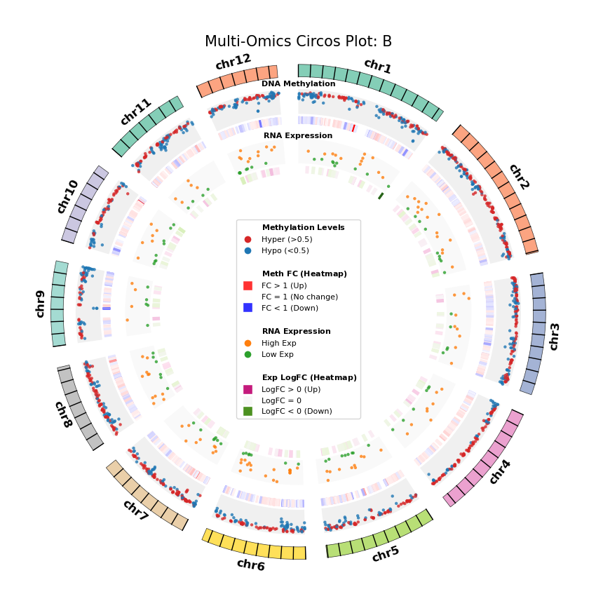

Functional Enrichment Analysis Overview

Functional enrichment analysis is used to identify the enrichment of Differentially Expressed Genes (DEGs) and Differentially Methylated Genes (DMGs) in biological functions, pathways, etc., helping to understand the biological significance of differential genes.

Analysis Content:

1. GO Enrichment Analysis: Identify Gene Ontology (GO) functional annotations enriched by differential genes.
   • GO_Biological_Process (BP): Biological Process.
   • GO_Cellular_Component (CC): Cellular Component.
   • GO_Molecular_Function (MF): Molecular Function.
2. KEGG Enrichment Analysis: Identify KEGG pathways enriched by differential genes.

Data Requirements:

• DEG.csv: Differentially expressed gene data, containing columns: cluster, names, scores, logfoldchanges, pvals, pvals_adj, pct_nz_group, pct_nz_reference.
• DMG.csv: Differentially methylated gene data, containing columns: names, pvals_adj, fc, AUROC, cluster.

💡 Note
This notebook uses the Python package gseapy for gene set functional enrichment analysis. Using gseapy allows automatic handling of gene sets, calling Enrichr or completing annotations based on local GOA/KEGG databases, and outputting standardized result tables and visualization charts.

Usage Suggestions

Please note the following before performing functional enrichment analysis:

• Prerequisites: It is recommended to complete differential analysis first and obtain DEG and DMG results before performing functional enrichment.
• Network Connection: Ensure a normal network connection as Enrichr API access is required.
• Gene Count: If the number of genes for a cell type is too small (< 5), the analysis for that cell type will be automatically skipped.
• Result Saving: Enrichment analysis results will be automatically saved to the specified output directory, including CSV tables and visualization images.

GO Functional Enrichment Analysis

# 1. Automatically Detect Table Type
def detect_table_type(df):
    """Automatically detect table type (DEG or DMG)"""
    if 'logfoldchanges' in df.columns:
        return 'DEG'
    elif 'fc' in df.columns:
        return 'DMG'
    else:
        raise ValueError("Cannot detect table type: missing logfoldchanges or fc column")

# 2. Preprocess Gene Names (DMG specific)
def clean_gene_name(gene):
    """Clean DMG gene names, extract gene name part"""
    if "_" in gene:
        return gene.split("_")[-1]
    return gene

# 3. Extract Gene List
def extract_genes(df, table_type, direction='up', logfc_cutoff=0.25, padj_cutoff=0.05):
    """Extract gene list from differential analysis results"""
    df = df.copy()

    if table_type == 'DEG':
        if direction == 'up':
            return df[(df['logfoldchanges'] > logfc_cutoff) & (df['pvals_adj'] < padj_cutoff)]['names'].tolist()
        elif direction == 'down':
            return df[(df['logfoldchanges'] < -logfc_cutoff) & (df['pvals_adj'] < padj_cutoff)]['names'].tolist()

    elif table_type == 'DMG':
        df['gene'] = df['names'].apply(clean_gene_name)
        if direction == 'up':
            return df[(df['fc'] > 1) & (df['pvals_adj'] < padj_cutoff)]['gene'].tolist()
        elif direction == 'down':
            return df[(df['fc'] < 1) & (df['pvals_adj'] < padj_cutoff)]['gene'].tolist()

    raise ValueError("direction must be up or down")

# 4. enrichr enrichment
def run_enrichr(gene_list, species, analysis_type):
    """Perform functional enrichment analysis using Enrichr"""
    sp = species.lower()

    if sp in ["human"]:
        kegg_lib = "KEGG_2021_Human"
    elif sp in ["mouse"]:
        kegg_lib = "KEGG_2019_Mouse"
    else:
        kegg_lib = "KEGG_2016"

    if analysis_type == 'GO':
        # Define each GO database separately
        go_databases = [
            'GO_Biological_Process_2025',
            'GO_Cellular_Component_2025',
            'GO_Molecular_Function_2025'
        ]
        
        # Call each database separately
        all_results = []
        for db_name in go_databases:
            try:
                enr = gp.enrichr(
                    gene_list=gene_list,
                    gene_sets=[db_name],
                    organism=species,
                    outdir=None
                )
                
                if enr is None or enr.results is None:
                    continue
                
                # Process returned results
                if isinstance(enr.results, pd.DataFrame):
                    df = enr.results.copy()
                elif isinstance(enr.results, dict):
                    if db_name in enr.results:
                        df = enr.results[db_name].copy()
                    else:
                        df = list(enr.results.values())[0].copy() if enr.results else pd.DataFrame()
                else:
                    continue
                
                if len(df) > 0:
                    df['Gene_set'] = db_name
                    all_results.append(df)
                    
            except Exception as e:
                print(f"Warning: {db_name} Analysis failed: {e}")
                continue
        
        # Merge all results
        if all_results:
            return pd.concat(all_results, ignore_index=True)
        else:
            return pd.DataFrame()
    
    elif analysis_type == 'KEGG':
        # KEGG has only one database, call directly
        enr = gp.enrichr(
            gene_list=gene_list,
            gene_sets=[kegg_lib],
            organism=species,
            outdir=None
        )
        
        if enr is None or enr.results is None:
            return pd.DataFrame()
        
        # Process returned results
        if isinstance(enr.results, pd.DataFrame):
            return enr.results
        elif isinstance(enr.results, dict):
            if kegg_lib in enr.results:
                return enr.results[kegg_lib]
            else:
                return list(enr.results.values())[0] if enr.results else pd.DataFrame()
        else:
            return pd.DataFrame()
    
    else:
        return pd.DataFrame()

# 5. Enrichment Entry Point
def run_enrichment(gene_list, species, analysis_type, method):
    """Enrichment analysis entry function"""
    if method != 'enrichr':
        raise ValueError("Current script only supports method='enrichr'")
    return run_enrichr(gene_list, species, analysis_type)

# 6. Loop Enrichment by Cell Type + Auto Plotting
def loop_enrichment(df, table_type, species='human', analysis_type='GO', method='enrichr',
                    direction='up', output_dir="./output", top_term=15, 
                    figsize=(4, 10), fontsize=6, dpi=300, max_term_length=50):
    """Loop enrichment analysis by cell type and auto plot"""
    os.makedirs(output_dir, exist_ok=True)
    all_results = []

    celltype_col = 'cluster'  # Both DEG and DMG tables use cluster column

    # Set matplotlib parameters
    plt.rcParams.update({
        'font.size': fontsize,
        'axes.titlesize': fontsize,
        'axes.labelsize': fontsize-3,
        'xtick.labelsize': fontsize - 1,
        'ytick.labelsize': fontsize-3,
        'legend.fontsize': fontsize - 1,
        'figure.dpi': dpi,
        'savefig.dpi': dpi,
    })

    for celltype, sub_df in df.groupby(celltype_col):
        gene_list = extract_genes(sub_df, table_type, direction=direction)

        if len(gene_list) < 5:
            continue

        try:
            res_df = run_enrichment(gene_list, species, analysis_type, method)
            
            if len(res_df) == 0:
                print(f"[WARNING] {celltype} {direction} No enrichment results, skipping")
                continue
            
            res_df['celltype'] = celltype
            res_df['direction'] = direction
            res_df['analysis_type'] = analysis_type
            all_results.append(res_df)

            # Auto plotting
            safe_name = str(celltype).replace("/", "_").replace(" ", "_")
            
            # Clean Term names
            res_df = res_df.copy()
            if 'Term' in res_df.columns:
                res_df['Term'] = res_df['Term'].str.split(" \(GO").str[0]
                res_df['Term'] = res_df['Term'].str.split(" \(REACTOME").str[0]
                res_df['Term'] = res_df['Term'].str.split(" \(KEGG").str[0]
                
                # Handle overly long term names
                def wrap_term(term, max_len=max_term_length):
                    if len(term) <= max_len:
                        return term
                    words = term.split()
                    lines = []
                    current_line = ""
                    for word in words:
                        test_line = current_line + " " + word if current_line else word
                        if len(test_line) <= max_len:
                            current_line = test_line
                        else:
                            if current_line:
                                lines.append(current_line)
                            current_line = word
                    if current_line:
                        lines.append(current_line)
                    return '\n'.join(lines) if len(lines) > 1 else term[:max_len-3] + '...'
                
                res_df['Term'] = res_df['Term'].apply(wrap_term)
            
            # Sort by p-value and take top N
            pval_col = 'Adjusted P-value' if 'Adjusted P-value' in res_df.columns else 'P-value'
            plot_df = res_df.sort_values(pval_col).head(top_term)
            
            dot_path = os.path.join(output_dir, f"{safe_name}_{direction}_dotplot.png")
            bar_path = os.path.join(output_dir, f"{safe_name}_{direction}_barplot.png")
            
            # Dotplot
            plt.figure(figsize=figsize, dpi=dpi)
            try:
                dotplot(plot_df, cmap='viridis_r', size=7, figsize=figsize, top_term=top_term)
                fig = plt.gcf()
                ax = plt.gca()
                fig.set_size_inches(figsize[0], figsize[1])
                ax.tick_params(axis='y', labelsize=fontsize)
                for label in ax.get_yticklabels():
                    label.set_fontsize(fontsize)
                ax.xaxis.label.set_fontsize(fontsize-3)
                ax.tick_params(axis='x', labelsize=fontsize-1)
                fig.savefig(dot_path, dpi=dpi, bbox_inches='tight', pad_inches=0.1)
            except Exception as e:
                print(f"Dotplot plotting failed {celltype}: {e}")
            finally:
                plt.close('all')

            # Barplot
            plt.figure(figsize=figsize, dpi=dpi)
            try:
                barplot(plot_df, cmap='viridis_r', size=4, color='darkred', figsize=figsize, top_term=top_term)
                fig = plt.gcf()
                ax = plt.gca()
                fig.set_size_inches(figsize[0], figsize[1])
                ax.tick_params(axis='y', labelsize=fontsize)
                for label in ax.get_yticklabels():
                    label.set_fontsize(fontsize)
                ax.xaxis.label.set_fontsize(fontsize-3)
                ax.tick_params(axis='x', labelsize=fontsize-1)
                fig.savefig(bar_path, dpi=dpi, bbox_inches='tight', pad_inches=0.1)
            except Exception as e:
                print(f"Barplot plotting failed {celltype}: {e}")
            finally:
                plt.close('all')

            print(f"[OK] {celltype} {direction} plots saved to {output_dir} (showing {len(plot_df)} terms)")

        except Exception as e:
            print(f"Enrichment failed {celltype}: {e}")
            import traceback
            traceback.print_exc()
            plt.close('all')

    return pd.concat(all_results, ignore_index=True) if all_results else pd.DataFrame()

# 7. Master Control Function
def run_full_pipeline(df, species='human', analysis_type='GO', method='enrichr',
                      direction='both', output_dir="./output", 
                      top_term=15, figsize=(4, 7), fontsize=10, dpi=300):
    """Functional enrichment analysis master control function"""
    table_type = detect_table_type(df)

    if direction == 'both':
        up = loop_enrichment(df, table_type, species, analysis_type, method,
                             direction='up', output_dir=output_dir, 
                             top_term=top_term, figsize=figsize, fontsize=fontsize, dpi=dpi)
        down = loop_enrichment(df, table_type, species, analysis_type, method,
                               direction='down', output_dir=output_dir,
                               top_term=top_term, figsize=figsize, fontsize=fontsize, dpi=dpi)

        results = []
        if not up.empty:
            results.append(up)
        if not down.empty:
            results.append(down)

        return pd.concat(results, ignore_index=True) if results else pd.DataFrame()

    else:
        return loop_enrichment(df, table_type, species, analysis_type, method,
                               direction=direction, output_dir=output_dir,
                               top_term=top_term, figsize=figsize, fontsize=fontsize, dpi=dpi)

print("Functional enrichment analysis function definition completed")

output

功能富集分析函数定义完成

What is GO Enrichment Analysis

Gene Ontology (GO) is a standardized vocabulary system describing gene functions. GO enrichment analysis is a commonly used functional annotation method to identify biological functions significantly enriched in a differential gene set.

Basic Principle of GO Enrichment Analysis:

• Compare the distribution of the differential gene set and the background gene set in a GO term using hypergeometric test or Fisher's exact test.
• Calculate p-value to evaluate whether differential genes are significantly enriched in that function.
• Use multiple testing correction (e.g., FDR) to control false positive rate.

Figure Legend: This figure shows the GO functional enrichment results of differential genes (Dotplot + Barplot).

• Dotplot: X-axis is Combined Score, Y-axis is GO term name (sorted by Adjusted P-value); dot size represents gene proportion (%Genes in set), color represents significance (log(Adjusted P-value), darker is more significant).
• Barplot: X-axis is Adjusted P-value (negative log), Y-axis is GO term name.
• Note: The figure displays Top 15 GO terms (BP/CC/MF) by default, all satisfying Adjusted P-value < 0.05.

# Read DEG data
df_deg = pd.read_csv(deg_file)
DEG_up_GO_dir = os.path.join(output_dir, "DEG", "GO_up_plots")
os.makedirs(DEG_up_GO_dir, exist_ok=True)
output_path = os.path.join(output_dir, "DEG")
os.makedirs(output_path, exist_ok=True)

# Execute GO enrichment analysis (Upregulated genes)
result = run_full_pipeline(
    df_deg, 
    output_dir=DEG_up_GO_dir,
    species=species,        # Species: 'human'=Human, 'mouse'=Mouse
    analysis_type='GO',     # 'GO', 'KEGG'
    method='enrichr',       # 'enrichr'
    direction='up'          # 'up', 'down', 'both'
)

# Save results
DEG_up_GO_file_path = os.path.join(output_path, "GO_up_enrichment.csv")
if not result.empty:
    result.to_csv(DEG_up_GO_file_path, index=False)
    print(f"DEG upregulated gene GO enrichment analysis completed, results saved to {DEG_up_GO_file_path}")
else:
    print("No significant results found for DEG upregulated gene GO enrichment analysis")

output

[OK] B up 图已保存到 ./enrichment_results/DEG/GO_up_plots (显示 15 个term)
[OK] CD14+ Mono up 图已保存到 ./enrichment_results/DEG/GO_up_plots (显示 15 个term)
[OK] CD8+ T up 图已保存到 ./enrichment_results/DEG/GO_up_plots (显示 15 个term)
[OK] DC up 图已保存到 ./enrichment_results/DEG/GO_up_plots (显示 15 个term)
[OK] FCGR3A+ Mono up 图已保存到 ./enrichment_results/DEG/GO_up_plots (显示 15 个term)
[OK] Memory CD4+ T up 图已保存到 ./enrichment_results/DEG/GO_up_plots (显示 15 个term)
[OK] NK up 图已保存到 ./enrichment_results/DEG/GO_up_plots (显示 15 个term)
[OK] Navie CD4+ T up 图已保存到 ./enrichment_results/DEG/GO_up_plots (显示 15 个term)
DEG上调基因GO富集分析完成，结果已保存到 ./enrichment_results/DEG/GO_up_enrichment.csv

High Expression Gene GO Functional Enrichment Analysis

Analyze GO functional enrichment of upregulated genes (logfoldchanges > 0.25, padj < 0.05) in Differentially Expressed Genes (DEGs).

# Define image display function (Markdown table version, compatible with VitePress)
def display_go_plots_html_table(output_dir):
    """Read saved dotplot/barplot images from output_dir, display using Markdown table to avoid HTML/Vue conflict"""
    from IPython.display import display as ipy_display, Markdown
    import base64
    import os
    import re
    import pandas as pd
    
    if not os.path.exists(output_dir):
        print(f"Directory does not exist: {output_dir}")
        return
    
    # Match filename format: celltype_direction_plot.png
    pattern = re.compile(r"^(.+)_(up|down)_(dotplot|barplot)\.png$")
    png_files = [f for f in os.listdir(output_dir) if f.endswith(".png")]
    
    if len(png_files) == 0:
        print(f"Warning: No PNG image files found in directory {output_dir}")
        print(f"Tip: Please ensure enrichment analysis code has run and image files were successfully generated")
        return
    
    # Structure: {celltype: {"dotplot": None, "barplot": None}}
    plot_dict = {}
    
    for f in png_files:
        m = pattern.match(f)
        if not m:
            continue
        
        celltype = m.group(1)
        plot_type = m.group(3)
        abs_path = os.path.join(output_dir, f)
        
        if celltype not in plot_dict:
            plot_dict[celltype] = {"dotplot": None, "barplot": None}
        
        plot_dict[celltype][plot_type] = abs_path
    
    if len(plot_dict) == 0:
        print(f"Warning: Found {len(png_files)} PNG files in directory {output_dir}, but none match expected format")
        return
    
    # Generate rows for Markdown table
    rows = []
    for celltype, plots in plot_dict.items():
        dot_html = "Image not found"
        bar_html = "Image not found"
        
        if plots["dotplot"] is not None and os.path.exists(plots["dotplot"]):
            with open(plots["dotplot"], "rb") as img_file:
                img_data = base64.b64encode(img_file.read()).decode()
                img_ext = os.path.splitext(plots["dotplot"])[1][1:]
                dot_html = f'<img src="/placeholder.svg" style="max-width: 100%; height: auto;" />'
        
        if plots["barplot"] is not None and os.path.exists(plots["barplot"]):
            with open(plots["barplot"], "rb") as img_file:
                img_data = base64.b64encode(img_file.read()).decode()
                img_ext = os.path.splitext(plots["barplot"])[1][1:]
                bar_html = f'<img src="/placeholder.svg" style="max-width: 100%; height: auto;" />'
        
        rows.append({
            "Cluster": celltype,
            "GO_dot": dot_html,
            "GO_bar": bar_html
        })
    
    rows.sort(key=lambda x: x["Cluster"])
    
    md_table = "| Cluster | GO_dot | GO_bar |\n| :--- | :--- | :--- |\n"
    for row in rows:
        md_table += f"| {row['Cluster']} | {row['GO_dot']} | {row['GO_bar']} |\n"
    
    ipy_display(Markdown(md_table))

Figure Legend: This figure shows the GO enrichment results for upregulated genes (logfoldchanges > 0.25, padj < 0.05); figure elements meaning see "GO Functional Enrichment Analysis Visualization Figure" legend above.

# Execute GO enrichment analysis (Downregulated genes)
df_deg = pd.read_csv(deg_file)
DEG_down_GO_dir = os.path.join(output_dir, "DEG", "GO_down_plots")
os.makedirs(DEG_down_GO_dir, exist_ok=True)

result = run_full_pipeline(
    df_deg, 
    output_dir=DEG_down_GO_dir,
    species=species,
    analysis_type='GO',
    method='enrichr',
    direction='down'
)

# Save results
DEG_down_GO_file_path = os.path.join(output_path, "GO_down_enrichment.csv")
if not result.empty:
    result.to_csv(DEG_down_GO_file_path, index=False)
    print(f"DEG downregulated gene GO enrichment analysis completed, results saved to {DEG_down_GO_file_path}")
else:
    print("No significant results found for DEG downregulated gene GO enrichment analysis")

output

[OK] B down 图已保存到 ./enrichment_results/DEG/GO_down_plots (显示 15 个term)
[OK] CD14+ Mono down 图已保存到 ./enrichment_results/DEG/GO_down_plots (显示 15 个term)
[OK] CD8+ T down 图已保存到 ./enrichment_results/DEG/GO_down_plots (显示 15 个term)
[OK] DC down 图已保存到 ./enrichment_results/DEG/GO_down_plots (显示 15 个term)
[OK] FCGR3A+ Mono down 图已保存到 ./enrichment_results/DEG/GO_down_plots (显示 15 个term)
[OK] Memory CD4+ T down 图已保存到 ./enrichment_results/DEG/GO_down_plots (显示 15 个term)
[OK] NK down 图已保存到 ./enrichment_results/DEG/GO_down_plots (显示 15 个term)
[OK] Navie CD4+ T down 图已保存到 ./enrichment_results/DEG/GO_down_plots (显示 15 个term)
DEG下调基因GO富集分析完成，结果已保存到 ./enrichment_results/DEG/GO_down_enrichment.csv

Low Expression Gene GO Functional Enrichment Analysis

Analyze GO functional enrichment of downregulated genes (logfoldchanges < -0.25, padj < 0.05) in Differentially Expressed Genes (DEGs).

# Display DEG downregulated gene GO enrichment results
if os.path.exists(DEG_down_GO_file_path):
    display_go_plots_html_table(DEG_down_GO_dir)

Figure Legend: This figure shows the GO enrichment results for downregulated genes (logfoldchanges < -0.25, padj < 0.05); figure elements meaning see "GO Functional Enrichment Analysis Visualization Figure" legend above.

# Read DMG data
df_dmg = pd.read_csv(dmg_file)
DMG_up_GO_dir = os.path.join(output_dir, "DMG", "GO_up_plots")
os.makedirs(DMG_up_GO_dir, exist_ok=True)
output_path_dmg = os.path.join(output_dir, "DMG")
os.makedirs(output_path_dmg, exist_ok=True)

# Execute GO enrichment analysis (Hypermethylated genes)
result = run_full_pipeline(
    df_dmg, 
    output_dir=DMG_up_GO_dir,
    species=species,
    analysis_type='GO',
    method='enrichr',
    direction='up'
)

# Save results
DMG_up_GO_file_path = os.path.join(output_path_dmg, "GO_up_enrichment.csv")
if not result.empty:
    result.to_csv(DMG_up_GO_file_path, index=False)
    print(f"DMG hypermethylated gene GO enrichment analysis completed, results saved to {DMG_up_GO_file_path}")
else:
    print("No significant results found for DMG hypermethylated gene GO enrichment analysis")

output

[OK] B up 图已保存到 ./enrichment_results/DMG/GO_up_plots (显示 15 个term)
[OK] CD14+ Mono up 图已保存到 ./enrichment_results/DMG/GO_up_plots (显示 15 个term)
[OK] CD8+ T up 图已保存到 ./enrichment_results/DMG/GO_up_plots (显示 15 个term)
[OK] DC up 图已保存到 ./enrichment_results/DMG/GO_up_plots (显示 15 个term)
[OK] FCGR3A+ Mono up 图已保存到 ./enrichment_results/DMG/GO_up_plots (显示 15 个term)
[OK] Memory CD4+ T up 图已保存到 ./enrichment_results/DMG/GO_up_plots (显示 15 个term)
Dotplot绘图失败 NK: Warning: No enrich terms when cutoff = 0.05
Barplot绘图失败 NK: Warning: No enrich terms when cutoff = 0.05
[OK] NK up 图已保存到 ./enrichment_results/DMG/GO_up_plots (显示 15 个term)
[OK] Navie CD4+ T up 图已保存到 ./enrichment_results/DMG/GO_up_plots (显示 15 个term)
DMG高甲基化基因GO富集分析完成，结果已保存到 ./enrichment_results/DMG/GO_up_enrichment.csv

Hypermethylated Gene GO Functional Enrichment Analysis

Analyze GO functional enrichment of hypermethylated genes (fc > 1, padj < 0.05) in Differentially Methylated Genes (DMGs).

💡 Note
The script automatically handles gene name formats in DMG data (e.g., ENSG00000128731_HERC2), extracting the gene name part (HERC2) for analysis.

# Display DMG hypermethylated gene GO enrichment results
if os.path.exists(DMG_up_GO_file_path):
    display_go_plots_html_table(DMG_up_GO_dir)

Figure Legend: This figure shows the GO enrichment results for hypermethylated genes (fc > 1, padj < 0.05); figure elements meaning see "GO Functional Enrichment Analysis Visualization Figure" legend above.

# Execute GO enrichment analysis (Hypomethylated genes)
df_dmg = pd.read_csv(dmg_file)
DMG_down_GO_dir = os.path.join(output_dir, "DMG", "GO_down_plots")
os.makedirs(DMG_down_GO_dir, exist_ok=True)

result = run_full_pipeline(
    df_dmg, 
    output_dir=DMG_down_GO_dir,
    species=species,
    analysis_type='GO',
    method='enrichr',
    direction='down'
)

# Save results
DMG_down_GO_file_path = os.path.join(output_path_dmg, "GO_down_enrichment.csv")
if not result.empty:
    result.to_csv(DMG_down_GO_file_path, index=False)
    print(f"DMG hypomethylated gene GO enrichment analysis completed, results saved to {DMG_down_GO_file_path}")
else:
    print("No significant results found for DMG hypomethylated gene GO enrichment analysis")

output

Dotplot绘图失败 B: Warning: No enrich terms when cutoff = 0.05
Barplot绘图失败 B: Warning: No enrich terms when cutoff = 0.05
[OK] B down 图已保存到 ./enrichment_results/DMG/GO_down_plots (显示 15 个term)
Dotplot绘图失败 CD14+ Mono: Warning: No enrich terms when cutoff = 0.05
Barplot绘图失败 CD14+ Mono: Warning: No enrich terms when cutoff = 0.05
[OK] CD14+ Mono down 图已保存到 ./enrichment_results/DMG/GO_down_plots (显示 15 个term)
[OK] CD8+ T down 图已保存到 ./enrichment_results/DMG/GO_down_plots (显示 15 个term)
[OK] DC down 图已保存到 ./enrichment_results/DMG/GO_down_plots (显示 15 个term)
Dotplot绘图失败 FCGR3A+ Mono: Warning: No enrich terms when cutoff = 0.05
Barplot绘图失败 FCGR3A+ Mono: Warning: No enrich terms when cutoff = 0.05
[OK] FCGR3A+ Mono down 图已保存到 ./enrichment_results/DMG/GO_down_plots (显示 15 个term)
[OK] Memory CD4+ T down 图已保存到 ./enrichment_results/DMG/GO_down_plots (显示 15 个term)
Dotplot绘图失败 NK: Warning: No enrich terms when cutoff = 0.05
Barplot绘图失败 NK: Warning: No enrich terms when cutoff = 0.05
[OK] NK down 图已保存到 ./enrichment_results/DMG/GO_down_plots (显示 15 个term)
[OK] Navie CD4+ T down 图已保存到 ./enrichment_results/DMG/GO_down_plots (显示 15 个term)
DMG低甲基化基因GO富集分析完成，结果已保存到 ./enrichment_results/DMG/GO_down_enrichment.csv

Hypomethylated Gene GO Functional Enrichment Analysis

Analyze GO functional enrichment of hypomethylated genes (fc < 1, padj < 0.05) in Differentially Methylated Genes (DMGs).

# Display DMG hypomethylated gene GO enrichment results
if os.path.exists(DMG_down_GO_file_path):
    display_go_plots_html_table(DMG_down_GO_dir)

Figure Legend: This figure shows the GO enrichment results for hypomethylated genes (fc < 1, padj < 0.05); figure elements meaning see "GO Functional Enrichment Analysis Visualization Figure" legend above.

KEGG Functional Enrichment Analysis

What is KEGG Functional Enrichment Analysis

KEGG (Kyoto Encyclopedia of Genes and Genomes) is a comprehensive database integrating genomic, chemical, and systemic functional information. KEGG enrichment analysis is used to identify biological pathways significantly enriched in differential gene sets.

Main Content of KEGG Database:

1. KEGG PATHWAY: Biological pathway maps, including metabolic pathways, signal transduction pathways, disease-related pathways, etc.
2. KEGG GENES: Functional annotation of genes and proteins.
3. KEGG COMPOUND: Compound database.
4. KEGG DISEASE: Disease-related pathways.

Basic Principle of KEGG Enrichment Analysis:

• Similar to GO enrichment analysis, compare the distribution of differential gene set and background gene set in a KEGG pathway using statistical tests (e.g., hypergeometric test).
• Identify biological pathways significantly enriched by differential genes.
• Help understand biological processes and pathway regulatory mechanisms involved by differential genes.

# Execute KEGG enrichment analysis (Upregulated genes)
df_deg = pd.read_csv(deg_file)
DEG_up_KEGG_dir = os.path.join(output_dir, "DEG", "KEGG_up_plots")
os.makedirs(DEG_up_KEGG_dir, exist_ok=True)

result = run_full_pipeline(
    df_deg, 
    output_dir=DEG_up_KEGG_dir,
    species=species,
    analysis_type='KEGG',
    method='enrichr',
    direction='up'
)

# Save results
DEG_up_KEGG_file_path = os.path.join(output_path, "KEGG_up_enrichment.csv")
if not result.empty:
    result.to_csv(DEG_up_KEGG_file_path, index=False)
    print(f"DEG upregulated gene KEGG enrichment analysis completed, results saved to {DEG_up_KEGG_file_path}")
else:
    print("No significant results found for DEG upregulated gene KEGG enrichment analysis")

output

[OK] B up 图已保存到 ./enrichment_results/DEG/KEGG_up_plots (显示 15 个term)
[OK] CD14+ Mono up 图已保存到 ./enrichment_results/DEG/KEGG_up_plots (显示 15 个term)
[OK] CD8+ T up 图已保存到 ./enrichment_results/DEG/KEGG_up_plots (显示 15 个term)
[OK] DC up 图已保存到 ./enrichment_results/DEG/KEGG_up_plots (显示 15 个term)
[OK] FCGR3A+ Mono up 图已保存到 ./enrichment_results/DEG/KEGG_up_plots (显示 15 个term)
[OK] Memory CD4+ T up 图已保存到 ./enrichment_results/DEG/KEGG_up_plots (显示 15 个term)
[OK] NK up 图已保存到 ./enrichment_results/DEG/KEGG_up_plots (显示 15 个term)
[OK] Navie CD4+ T up 图已保存到 ./enrichment_results/DEG/KEGG_up_plots (显示 15 个term)
DEG上调基因KEGG富集分析完成，结果已保存到 ./enrichment_results/DEG/KEGG_up_enrichment.csv

Figure Legend: This figure shows the KEGG pathway enrichment results of differential genes (Dotplot + Barplot).

• Dotplot: X-axis is Combined Score, Y-axis is KEGG pathway name (sorted by Adjusted P-value); dot size represents gene proportion (%Genes in set), color represents significance (log(Adjusted P-value), darker is more significant).
• Barplot: X-axis is Adjusted P-value (negative log), Y-axis is KEGG pathway name.
• Note: The figure displays Top 15 pathways by default, all satisfying Adjusted P-value < 0.05; pathway IDs (e.g., hsa04010) can be queried on the KEGG website for details.

# Display DEG upregulated gene KEGG enrichment results
if os.path.exists(DEG_up_KEGG_file_path):
    display_go_plots_html_table(DEG_up_KEGG_dir)

High Expression Gene KEGG Functional Enrichment Analysis

Analyze KEGG pathway enrichment of upregulated genes (logfoldchanges > 0.25, padj < 0.05) in Differentially Expressed Genes (DEGs).

# Execute KEGG enrichment analysis (Downregulated genes)
df_deg = pd.read_csv(deg_file)
DEG_down_KEGG_dir = os.path.join(output_dir, "DEG", "KEGG_down_plots")
os.makedirs(DEG_down_KEGG_dir, exist_ok=True)

result = run_full_pipeline(
    df_deg, 
    output_dir=DEG_down_KEGG_dir,
    species=species,
    analysis_type='KEGG',
    method='enrichr',
    direction='down'
)

# Save results
DEG_down_KEGG_file_path = os.path.join(output_path, "KEGG_down_enrichment.csv")
if not result.empty:
    result.to_csv(DEG_down_KEGG_file_path, index=False)
    print(f"DEG downregulated gene KEGG enrichment analysis completed, results saved to {DEG_down_KEGG_file_path}")
else:
    print("No significant results found for DEG downregulated gene KEGG enrichment analysis")

output

[OK] B down 图已保存到 ./enrichment_results/DEG/KEGG_down_plots (显示 15 个term)
[OK] CD14+ Mono down 图已保存到 ./enrichment_results/DEG/KEGG_down_plots (显示 15 个term)
[OK] CD8+ T down 图已保存到 ./enrichment_results/DEG/KEGG_down_plots (显示 15 个term)
[OK] DC down 图已保存到 ./enrichment_results/DEG/KEGG_down_plots (显示 15 个term)
[OK] FCGR3A+ Mono down 图已保存到 ./enrichment_results/DEG/KEGG_down_plots (显示 15 个term)
[OK] Memory CD4+ T down 图已保存到 ./enrichment_results/DEG/KEGG_down_plots (显示 15 个term)
[OK] NK down 图已保存到 ./enrichment_results/DEG/KEGG_down_plots (显示 15 个term)
[OK] Navie CD4+ T down 图已保存到 ./enrichment_results/DEG/KEGG_down_plots (显示 15 个term)
DEG下调基因KEGG富集分析完成，结果已保存到 ./enrichment_results/DEG/KEGG_down_enrichment.csv

Figure Legend: This figure shows the KEGG pathway enrichment results for upregulated genes (logfoldchanges > 0.25, padj < 0.05); figure elements meaning see "KEGG Functional Enrichment Analysis Visualization Figure" legend above.

# Display DEG downregulated gene KEGG enrichment results
if os.path.exists(DEG_down_KEGG_file_path):
    display_go_plots_html_table(DEG_down_KEGG_dir)

Low Expression Gene KEGG Functional Enrichment Analysis

Analyze KEGG pathway enrichment of downregulated genes (logfoldchanges < -0.25, padj < 0.05) in Differentially Expressed Genes (DEGs).

# Execute KEGG enrichment analysis (Hypermethylated genes)
df_dmg = pd.read_csv(dmg_file)
DMG_up_KEGG_dir = os.path.join(output_dir, "DMG", "KEGG_up_plots")
os.makedirs(DMG_up_KEGG_dir, exist_ok=True)

result = run_full_pipeline(
    df_dmg, 
    output_dir=DMG_up_KEGG_dir,
    species=species,
    analysis_type='KEGG',
    method='enrichr',
    direction='up'
)

# Save results
DMG_up_KEGG_file_path = os.path.join(output_path_dmg, "KEGG_up_enrichment.csv")
if not result.empty:
    result.to_csv(DMG_up_KEGG_file_path, index=False)
    print(f"DMG hypermethylated gene KEGG enrichment analysis completed, results saved to {DMG_up_KEGG_file_path}")
else:
    print("No significant results found for DMG hypermethylated gene KEGG enrichment analysis")

output

Dotplot绘图失败 B: Warning: No enrich terms when cutoff = 0.05
Barplot绘图失败 B: Warning: No enrich terms when cutoff = 0.05
[OK] B up 图已保存到 ./enrichment_results/DMG/KEGG_up_plots (显示 15 个term)
[OK] CD14+ Mono up 图已保存到 ./enrichment_results/DMG/KEGG_up_plots (显示 15 个term)
Dotplot绘图失败 CD8+ T: Warning: No enrich terms when cutoff = 0.05
Barplot绘图失败 CD8+ T: Warning: No enrich terms when cutoff = 0.05
[OK] CD8+ T up 图已保存到 ./enrichment_results/DMG/KEGG_up_plots (显示 15 个term)
Dotplot绘图失败 DC: Warning: No enrich terms when cutoff = 0.05
Barplot绘图失败 DC: Warning: No enrich terms when cutoff = 0.05
[OK] DC up 图已保存到 ./enrichment_results/DMG/KEGG_up_plots (显示 15 个term)
Dotplot绘图失败 FCGR3A+ Mono: Warning: No enrich terms when cutoff = 0.05
Barplot绘图失败 FCGR3A+ Mono: Warning: No enrich terms when cutoff = 0.05
[OK] FCGR3A+ Mono up 图已保存到 ./enrichment_results/DMG/KEGG_up_plots (显示 15 个term)
Dotplot绘图失败 Memory CD4+ T: Warning: No enrich terms when cutoff = 0.05
Barplot绘图失败 Memory CD4+ T: Warning: No enrich terms when cutoff = 0.05
[OK] Memory CD4+ T up 图已保存到 ./enrichment_results/DMG/KEGG_up_plots (显示 15 个term)
Dotplot绘图失败 NK: Warning: No enrich terms when cutoff = 0.05
Barplot绘图失败 NK: Warning: No enrich terms when cutoff = 0.05
[OK] NK up 图已保存到 ./enrichment_results/DMG/KEGG_up_plots (显示 15 个term)
Dotplot绘图失败 Navie CD4+ T: Warning: No enrich terms when cutoff = 0.05
Barplot绘图失败 Navie CD4+ T: Warning: No enrich terms when cutoff = 0.05
[OK] Navie CD4+ T up 图已保存到 ./enrichment_results/DMG/KEGG_up_plots (显示 15 个term)
DMG高甲基化基因KEGG富集分析完成，结果已保存到 ./enrichment_results/DMG/KEGG_up_enrichment.csv

Figure Legend: This figure shows the KEGG pathway enrichment results for downregulated genes (logfoldchanges < -0.25, padj < 0.05); figure elements meaning see "KEGG Functional Enrichment Analysis Visualization Figure" legend above.

# Display DMG hypermethylated gene KEGG enrichment results
if os.path.exists(DMG_up_KEGG_file_path):
    display_go_plots_html_table(DMG_up_KEGG_dir)

Hypermethylated Gene KEGG Functional Enrichment Analysis

Analyze KEGG pathway enrichment of hypermethylated genes (fc > 1, padj < 0.05) in Differentially Methylated Genes (DMGs).

# Execute KEGG enrichment analysis (Hypomethylated genes)
df_dmg = pd.read_csv(dmg_file)
DMG_down_KEGG_dir = os.path.join(output_dir, "DMG", "KEGG_down_plots")
os.makedirs(DMG_down_KEGG_dir, exist_ok=True)

result = run_full_pipeline(
    df_dmg, 
    output_dir=DMG_down_KEGG_dir,
    species=species,
    analysis_type='KEGG',
    method='enrichr',
    direction='down'
)

# Save results
DMG_down_KEGG_file_path = os.path.join(output_path_dmg, "KEGG_down_enrichment.csv")
if not result.empty:
    result.to_csv(DMG_down_KEGG_file_path, index=False)
    print(f"DMG hypomethylated gene KEGG enrichment analysis completed, results saved to {DMG_down_KEGG_file_path}")
else:
    print("No significant results found for DMG hypomethylated gene KEGG enrichment analysis")

output

[OK] B down 图已保存到 ./enrichment_results/DMG/KEGG_down_plots (显示 15 个term)
Dotplot绘图失败 CD14+ Mono: Warning: No enrich terms when cutoff = 0.05
Barplot绘图失败 CD14+ Mono: Warning: No enrich terms when cutoff = 0.05
[OK] CD14+ Mono down 图已保存到 ./enrichment_results/DMG/KEGG_down_plots (显示 15 个term)
Dotplot绘图失败 CD8+ T: Warning: No enrich terms when cutoff = 0.05
Barplot绘图失败 CD8+ T: Warning: No enrich terms when cutoff = 0.05
[OK] CD8+ T down 图已保存到 ./enrichment_results/DMG/KEGG_down_plots (显示 15 个term)
Dotplot绘图失败 DC: Warning: No enrich terms when cutoff = 0.05
Barplot绘图失败 DC: Warning: No enrich terms when cutoff = 0.05
[OK] DC down 图已保存到 ./enrichment_results/DMG/KEGG_down_plots (显示 15 个term)
Dotplot绘图失败 FCGR3A+ Mono: Warning: No enrich terms when cutoff = 0.05
Barplot绘图失败 FCGR3A+ Mono: Warning: No enrich terms when cutoff = 0.05
[OK] FCGR3A+ Mono down 图已保存到 ./enrichment_results/DMG/KEGG_down_plots (显示 15 个term)
Dotplot绘图失败 Memory CD4+ T: Warning: No enrich terms when cutoff = 0.05
Barplot绘图失败 Memory CD4+ T: Warning: No enrich terms when cutoff = 0.05
[OK] Memory CD4+ T down 图已保存到 ./enrichment_results/DMG/KEGG_down_plots (显示 15 个term)
[OK] NK down 图已保存到 ./enrichment_results/DMG/KEGG_down_plots (显示 15 个term)
[OK] Navie CD4+ T down 图已保存到 ./enrichment_results/DMG/KEGG_down_plots (显示 15 个term)
DMG低甲基化基因KEGG富集分析完成，结果已保存到 ./enrichment_results/DMG/KEGG_down_enrichment.csv

Figure Legend: This figure shows the KEGG pathway enrichment results for hypermethylated genes (fc > 1, padj < 0.05); figure elements meaning see "KEGG Functional Enrichment Analysis Visualization Figure" legend above.

# Display DMG hypomethylated gene KEGG enrichment results
if os.path.exists(DMG_down_KEGG_file_path):
    display_go_plots_html_table(DMG_down_KEGG_dir)