scMethyl + RNA Multi-omics: Integration Analysis Tutorial Based on MOFA+ Algorithm

Author: SeekGene

Time: 39 min

Words: 7.6k words

Updated: 2026-03-30

Reads: 0 times

scMethyl + RNA-seq Notebooks

Module Introduction

This tutorial details how to use the MOFA+ (Multi-Omics Factor Analysis v2) framework for multi-omics integration analysis of single-cell methylation (DNA Methylation) and transcriptome (RNA) data.

MOFA+ Analysis Principles

MOFA+ is an unsupervised statistical framework designed to infer latent low-dimensional factors (Latent Factors) from multi-omics data. Its core idea is to decompose data from different omics modalities (Views) into a set of shared or private latent factors.

• Input Data: Matrices containing multiple omics modalities (such as RNA and DNA Methylation), where rows represent aligned cells and columns represent their respective features (genes or methylation regions).
• Latent Factors: The model extracts low-dimensional factors driving data variation through matrix factorization.
  • Shared Factors: Capture biological variation co-existing in multiple omics modalities (such as cell type, cell cycle, etc.), explaining the variance of both RNA and methylation data simultaneously.
  • Private Factors: Capture variation existing only in a single omics modality (such as technical noise specific to one omics, batch effects, or specific biological signals).
• Model Reconstruction: The data is decomposed into the product of a Factor Matrix and a Weight Matrix. The weight matrix measures the contribution of each feature to a specific factor.
• Sparsity: MOFA+ introduces sparsity priors, so each factor is associated with only a small number of key features (genes or methylation regions). This regularization not only prevents overfitting but also significantly improves the biological interpretability of the model.

Analysis Objectives

1. Multi-omics Dimensionality Reduction: Compress high-dimensional RNA and methylation data into a small number of latent factors, retaining the main biological variation.
2. Variance Explanation: Quantify and assess the contribution of each factor to the overall variance of different omics modalities (Variance Explained).
3. Joint Clustering: Construct a neighbor graph based on the extracted low-dimensional factor space for more robust joint dimensionality reduction (UMAP) and cell clustering (Leiden).

Preparation

Import Dependencies and Define Helper Functions

This section primarily completes the following tasks:

1. Import Analysis Libraries: Including standard single-cell analysis libraries (scanpy, muon), methylation analysis library (ALLCools), and plotting library (matplotlib).
2. Define Data Loading and Processing Functions:
   • mcds_to_adata: Convert MCDS format (methylation storage format) to AnnData object.
   • mcds_get_mc_frac_adata: Read and process Methylation Fraction matrix, supporting blacklist region filtering and highly variable feature calculation.
   • compute_cg_ch_level: Calculate global CG and CH methylation levels for each cell.
   • check_barcode_overlap: Check cell Barcode overlap between RNA and Methylation data to ensure multi-omics data comes from the same batch of cells.
   • parse_gtf: Parse GTF annotation file to extract gene type information.

import os
# Set environment variables to ensure the correct conda environment and binaries are used
os.environ['PATH'] =  "/PROJ/home/weiqiuxia/micromamba/envs/muon_env/bin:/opt/conda/bin:/opt/conda/condabin:/usr/local/sbin:/usr/local/bin:/usr/sbin:/usr/bin:/sbin:/bin:/PROJ2/FLOAT/public/bin"
r_base_path = '/PROJ/home/weiqiuxia/micromamba/envs/muon_env'
os.environ['R_HOME'] = os.path.join(r_base_path, 'lib', 'R')    
# Set shared library path
os.environ['LD_LIBRARY_PATH'] = os.path.join(r_base_path, 'lib', 'R', 'lib') + ':' + os.environ.get('LD_LIBRARY_PATH', '')
# Set R library paths
r_lib_path = os.path.join(r_base_path, 'lib', 'R', 'library')
os.environ['R_LIBS'] = r_lib_path
os.environ['R_LIBS_USER'] = r_lib_path
os.environ['R_LIBS_SITE'] = r_lib_path

import re
import glob
from ALLCools.mcds import MCDS 
from ALLCools.clustering import tsne, significant_pc_test, log_scale, lsi, binarize_matrix, filter_regions, cluster_enriched_features, ConsensusClustering, Dendrogram, get_pc_centers
from ALLCools.clustering.doublets import MethylScrublet
from ALLCools.plot import *
import scanpy as sc 
import scanpy.external as sce
from harmonypy import run_harmony 
import numpy as np
import pandas as pd
import matplotlib.pyplot as plt
import matplotlib.colors as mcolors
from matplotlib.lines import Line2D
import warnings
import xarray as xr
from ALLCools.clustering import one_vs_rest_dmg
from scipy import sparse
import muon as mu 
from muon import atac as ac
from skmisc.loess import loess
import mofax as mfx 
import re
from collections import defaultdict

sc.settings.verbosity = 0
warnings.filterwarnings('ignore')

try:
    from matplotlib_venn import venn2
    HAS_VENN = True
except Exception:
    HAS_VENN = False

plt.rcParams['figure.dpi'] = 80  
plt.rcParams['savefig.dpi'] = 300      
plt.rcParams['figure.figsize'] = (5,5)

def mcds_to_adata(mcds_path, var_dim = 'chrom20k', mc_type = 'CGN', quant_type = 'hypo-score'):
    '''
    Convert the hypo-score matrix to an AnnData object
    '''
    # Read MCDS file
    mcds = MCDS.open(mcds_path, obs_dim = 'cell', var_dim = var_dim)
    # Get the score matrix and convert to AnnData
    adata = mcds.get_score_adata(mc_type=mc_type, quant_type=quant_type, sparse = True)
    return(adata)

def mcds_get_mc_frac_adata(mcds_path, var_dim = 'chrom20k', mc_type = 'CGN', obs_dim = 'cell',
                           min_cov = 1, met_matrix_type = 'mc_frac', hvf_method='SVR' ,n_top_feature = 2000, 
                           clip_norm_value = 10,
                           black_list_path = None, ):
    '''
    Convert the methylation fraction matrix or M-value matrix to an AnnData object
    '''
    # 1. Open MCDS dataset
    mcds = MCDS.open(
        mcds_path, 
        obs_dim = 'cell', 
        var_dim = var_dim
    )
    # 2. Compute mean coverage per feature (Coverage Mean)
    if "mc_type" in mcds[f'{var_dim}_da'].dims:
        feature_cov_mean = mcds.sel(count_type="cov").sum(dim="mc_type").mean(dim=obs_dim).squeeze().to_pandas()
    else:
        feature_cov_mean = mcds[f'{var_dim}_da'].sel(count_type="cov").mean(dim=obs_dim).squeeze().to_pandas()
        
    mcds.coords[f'{var_dim}_cov_mean'] = (var_dim, feature_cov_mean)
    # Filter out low-coverage features
    mcds = mcds.filter_feature_by_cov_mean(min_cov=min_cov)
    
    # 3. (Optional) Remove blacklist regions (Blacklist Regions)
    if black_list_path:
        mcds = mcds.remove_black_list_region(
            black_list_path = black_list_path,
            f = 0.2
        )
    load = True
    obs_dim = 'cell'
    # 4. Compute methylation matrix (M-value or Methylation Fraction)
    if met_matrix_type == 'mvalue':
        mcds.add_m_value(var_dim=var_dim)
        da_suffix = 'mvalue'
    else:
        if met_matrix_type == 'mc_frac':
            mcds.add_mc_frac(var_dim=var_dim,clip_norm_value=clip_norm_value,normalize_per_cell=True)
        else:
            clip_norm_value = None
            mcds.add_mc_frac(var_dim=var_dim,clip_norm_value=clip_norm_value,normalize_per_cell=False)
        da_suffix = 'frac'
    
    # Load data into memory
    if load and (mcds.get_index(obs_dim).size < 20000):
        mcds[f'{var_dim}_da_{da_suffix}'].load()
        
    # 5. Compute highly variable features (Highly Variable Features)
    if hvf_method == 'SVR':
        mcg_hvf = mcds.calculate_hvf_svr(
        var_dim = var_dim,
        mc_type = mc_type,
        da_suffix = da_suffix,
        n_top_feature = n_top_feature,
        plot = False)
    else:
        mcg_hvf = mcds.calculate_hvf(
        var_dim = var_dim,
        mc_type = mc_type,
        da_suffix = da_suffix,
        n_top_feature = n_top_feature,
        plot = False)
        
    # 6. Create AnnData object and merge HVF metadata
    mcg_adata = mcds.get_adata(
    mc_type=mc_type,
    var_dim = var_dim,
    select_hvf = True,
    da_suffix = da_suffix)
    mcg_adata.var = mcg_adata.var.merge(mcg_hvf, right_index = True, left_index = True)
    return mcg_adata
    
def compute_cg_ch_level(df):
    '''
    Compute CG and CH methylation levels
    ''' 
    # Select coverage (cov) and methylation (mc) columns for CG and CH contexts
    cg_cov_col = [i for i in df.columns[df.columns.str.startswith('CG')].to_list() if i.endswith('_cov')]
    cg_mc_col = [i for i in df.columns[df.columns.str.startswith('CG')].to_list() if i.endswith('_mc')]
    ch_cov_col = [i for i in df.columns[df.columns.str.contains('^(CT|CC|CA)')].to_list() if i.endswith('_cov')]
    ch_mc_col = [i for i in df.columns[df.columns.str.contains('^(CT|CC|CA)')].to_list() if i.endswith('_mc')]
    
    # Compute global CG methylation fraction
    df['CpG_cov'] = df[cg_cov_col].sum(axis=1)
    df['CpG_mc'] = df[cg_mc_col].sum(axis=1)
    df['CpG%'] = round(df['CpG_mc'] * 100 / df['CpG_cov'], 2)
    
    # Compute global CH methylation fraction
    df['CH_cov'] = df[ch_cov_col].sum(axis=1)
    df['CH_mc'] = df[ch_mc_col].sum(axis=1)
    df['CH%'] = round(df['CH_mc'] * 100 / df['CH_cov'], 2)

    return df

def check_barcode_overlap(rna_adata, met_adata, barcode_map = None):
    '''
    Check barcode overlap between transcriptome and methylation data, and reset RNA barcodes to the corresponding methylation barcodes.
    '''
    # Compute barcode overlap rate
    rna_adata.obs['original_barcode'] = [ re.sub('_.*', '', i) for i in rna_adata.obs.index ]
    met_adata.obs['original_barcode'] = [ re.sub('_.*', '', i) for i in met_adata.obs.index ]
    overlap_rate = len(set(rna_adata.obs['original_barcode']) & set(met_adata.obs['original_barcode'])) / met_adata.shape[0]
    
    # If overlap rate is low (<10%), try converting barcodes using the mapping table
    if overlap_rate < 0.1:
        met2rna_barcode = barcode_map[barcode_map['m_cb'].isin(met_adata.obs['original_barcode'])]
        rna_adata = rna_adata[rna_adata.obs['original_barcode'].obs.index.isin(met2rna_barcode['gex_cb'])]
        met2rna_barcode = met2rna_barcode.set_index('gex_cb')
        rna_adata.obs['gex_cb'] = rna_adata.obs.index
        rna_adata.obs.index = met2rna_barcode.loc[rna_adata.obs['original_barcode'],'m_cb']
        
        # Re-check overlap rate
        overlap_rate_test = len(set(rna_adata.obs.index) & set(met_adata.obs.index)) / met_adata.shape[0]
        chemistry = 'DD-MET3'
        if overlap_rate_test < 0.1:
            raise Exception('The overlap rate between RNA data and MET data barcode is less than 10%')
    else:
        chemistry = 'DD-MET5'
        rna_adata.obs.index = rna_adata.obs['original_barcode']
        met_adata.obs.index = met_adata.obs['original_barcode']
        
    # Keep only cells shared by both modalities
    common_index = list(set(rna_adata.obs.index) & set(met_adata.obs.index))
    rna_adata = rna_adata[rna_adata.obs.index.isin(common_index)]
    rna_adata.obs['chemistry'] = chemistry
    met_adata = met_adata[met_adata.obs.index.isin(common_index)]
    met_adata.obs['chemistry'] = chemistry
    return rna_adata, met_adata, chemistry 


def parse_gtf(gtf_file, output_file):
    '''
    Read GTF, get gene_type information for genes.
    '''
    with open(gtf_file, 'r') as f_in, open(output_file, 'w') as f_out:
        for line in f_in:
            if line.startswith('#'):
                continue
            parts = line.strip().split('\t')
            if len(parts) < 9:
                continue
            
            feature_type = parts[2]
            if feature_type != 'gene':
                continue
            
            attributes = parts[8]
            attr_dict = {}
            # Basic parsing of GTF attributes: key "value"; key "value";
            for attr in attributes.split(';'):
                attr = attr.strip()
                if not attr:
                    continue
                if ' ' in attr:
                    key, value = attr.split(' ', 1)
                    value = value.strip('"')
                    attr_dict[key] = value
            
            gene_id = attr_dict.get('gene_id', '')
            gene_name = attr_dict.get('gene_name', '')
            gene_type = attr_dict.get('gene_type', '')
            
            # Construct the first column
            if gene_id and gene_name:
                col1 = f"{gene_id}_{gene_name}"
            elif gene_id:
                col1 = gene_id
            else:
                col1 = gene_name # Should not happen based on GTF spec but good to handle
                
            f_out.write(f"{col1}\t{gene_type}\n")

def rds_to_matrix(filepath, outdir):
    import rpy2.robjects as robjects
    robjects.globalenv['rdsfile'] = filepath
    robjects.globalenv['outdir'] = outdir
    
    print(f"R_HOME: {os.environ['R_HOME']}")
    print(f"R_LIBS: {os.environ['R_LIBS']}")
    print(f"LD_LIBRARY_PATH: {os.environ['LD_LIBRARY_PATH']}")
    # Run R code and retrieve results
    robjects.r('''
    library(Seurat)
    library(qs)
    if(endsWith(rdsfile, ".rds")){
        obj <- readRDS(rdsfile)
    }else{
        obj <- qread(rdsfile)
    }
    dir.create(outdir, recursive = TRUE)

    Matrix::writeMM(GetAssayData(obj, assay = "RNA", layer = "counts"), file = file.path(outdir, "matrix.mtx") )
    cmd <- paste0("gzip ", file.path(outdir, "matrix.mtx"))
    system(cmd)
    
    features <- data.frame(Feature_id = rownames(obj), Feature_name = rownames(obj), Feature_type = "Gene Expression")
    write.table(features, file.path(outdir, "features.tsv"), row.names = F, col.names = F, sep = "\t", quote = F)
    cmd <- paste0("gzip ", file.path(outdir, "features.tsv"))
    system(cmd)
    
    
    barcodes <- data.frame(Barcode = colnames(obj))
    write.table(barcodes, file.path(outdir, "barcodes.tsv"), row.names = F, col.names = F, sep = "\t", quote = F)
    cmd <- paste0("gzip ", file.path(outdir, "barcodes.tsv"))
    system(cmd)

    meta <- obj@meta.data
    write.table(tibble::rownames_to_column(meta, "barcode"), file.path(outdir, "meta.csv"), row.names = FALSE, col.names = TRUE, sep = ",", quote = F)
    
''')

Input Directory Structure Description

Important Note: This workflow has specific requirements for the input directory structure. The program will automatically retrieve RNA and methylation-related input files based on the indir parameter. It is recommended to organize the data as follows:

data/AY1768874914782/ (indir)
├── input.rds                                          # Transcriptome data (Seurat object or qs format)
└── methylation                                        # Methylation data root directory 
    └── demoWTJW969-task-1                             # Task/Batch name
        └── WTJW969                                    # Sample name
            ├── allcools_generate_datasets
            │   └── WTJW969.mcds                       # MCDS dataset folder
            │       ├── chrom100k
            │       ├── chrom10k
            │       ├── chrom20k                       # Methylation score matrix for 20kb windows
            │       └── ...
            └── split_bams
                ├── filtered_barcode_reads_counts.csv  # Filtered Barcode mapped reads counts
                └── WTJW969_cells.csv                  # Filtered cell QC information (CpG count, coverage, etc.)

• RNA Data Retrieval: Match .rds or .qs files under the indir path.
• Methylation Data Retrieval: Retrieve MCDS files and associated QC CSV files under the indir/methylation path.

# indir: input directory
indir = '/home/weiqiuxia/workspace/data/AY1768874914782/'
# outdir: output directory for results
outdir = '/home/weiqiuxia/workspace/project/weiqiuxia/MOFA_results'
# dd_met3_barcode_map: barcode mapping table for DD-MET3
dd_met3_barcode_map = '/home/weiqiuxia/workspace/project/weiqiuxia/DD-M_bUCB3_whitelist.csv'
# black_list_path: regions to filter (BED). Regions with 20% overlap will be removed from methylation features
black_list_path = '/home/weiqiuxia/workspace/project/weiqiuxia/hg38-blacklist-sort.v2.bed'
# resolution: clustering resolution for methylation (float > 0)
resolution = 1
# anno_col: cell annotation column name in RNA metadata
anno_col = 'CellAnnotation'
# sample_col: sample column name (default `Sample`); should match sample names under `indir`
sample_col = 'Sample'
# rna_n_top_feature: number of highly variable genes for RNA
rna_n_top_feature = 2000
# matrix_type: methylation matrix type. Options: hypo-score | mvalue
met_matrix_type = 'mvalue'
# var_dim: methylation feature dimension(s). Multiple values are allowed
var_dim = ['geneslop2k']
# total_cpg_number_cutoff: CpG count cutoff
total_cpg_number_cutoff = 500
# mc_type: methylation type: CGN. Currently only CGN is supported
mc_type = 'CGN'
# min_cov: filter out features with mean coverage below this value
min_cov = 10
# normalize_per_cell: whether to use posterior estimation for methylation fraction. True denoises/implicates; False uses raw methylation levels
normalize_per_cell=True
# met_n_top_feature: method for selecting highly variable features. Possible values: SVR | Based
hvf_method='SVR'
# met_n_top_feature: number of highly variable features to select for methylation
met_n_top_feature = 2500
# total_cpg_number_cutoff: CpG count cutoff
total_cpg_number_cutoff = 500

os.makedirs(outdir, exist_ok=True)

# Read DD-MET3 barcode mapping table
dd_met3_barcode_map_df = pd.read_csv(dd_met3_barcode_map, header = 0)

# First locate the input .qs/.rds file, convert it to a matrix, then load with scanpy
for i in os.listdir(indir):
    if i.endswith('.qs'):
        rds_to_matrix(os.path.join(indir, i), os.path.join(outdir, 'input_matrix'))
        break

output

R_HOME: /PROJ/home/weiqiuxia/micromamba/envs/muon_env/lib/R
R_LIBS: /PROJ/home/weiqiuxia/micromamba/envs/muon_env/lib/R/library
LD_LIBRARY_PATH: /PROJ/home/weiqiuxia/micromamba/envs/muon_env/lib/R/lib:

# Load RNA data with scanpy
adata_rna = sc.read_10x_mtx(f'{outdir}/input_matrix/')
meta = pd.read_csv(f'{outdir}/input_matrix/meta.csv', index_col = 0, header = 0)
adata_rna.obs = meta
adata_rna.obs['CellAnnotation'] = adata_rna.obs['CellAnnotation'].astype('category')

Methylation Data Preprocessing

Single-cell methylation data is highly sparse and has distinct signal distribution characteristics, so specific preprocessing strategies are needed for the specified methylation matrix type (met_matrix_type) to ensure downstream analysis accuracy.

We support the following two common data types and their corresponding processing workflows:

• Hypo-score Matrix:

  • Binarization: Use binarize_matrix function to convert continuous Hypo-score to binary signals. We consider sites with hypo-score > 0.95 as significantly hypomethylated (labeled as 1), and the rest as background (labeled as 0). This helps reduce technical noise and highlight biological signals.
  • TF-IDF Transformation: Apply TF-IDF (Term Frequency-Inverse Document Frequency) algorithm. This is a standard method for handling sparse binary data (similar to scATAC-seq analysis), effectively correcting sequencing depth differences and reducing the weight of ubiquitous features to extract cell-specific information.

• M-value Matrix:

  • Logit Transformation: Based on raw Methylation Fraction, calculate M-value using the formula np.log2((frac + alpha) / (1 - frac + alpha)). This transformation maps the [0, 1] methylation rate interval to the real number domain, providing better variance stability, making it more suitable for linear models and dimensionality reduction analysis.

Subsequently, we will perform Feature Selection based on the processed matrix, screening for methylation regions with the largest variation across cells, to prepare for subsequent multi-modal integration.

# Load methylation data and take the intersection with transcriptome data to ensure cells and barcodes match
keep_col = ['barcode', 'total_cpg_number', 'genome_cov', 'reads_counts', 'CpG%', 'CH%']
obj_met_list = defaultdict(defaultdict)
obj_rna_list = defaultdict()
indirs = indir.split(',')
samples = []
mcds_paths = {}
sample_path = {}
analysis_batch_dir = os.listdir(os.path.join(indir, 'methylation'))
for i in analysis_batch_dir:
    if os.path.isdir(os.path.join(indir, 'methylation', i)):
        a_batch_dir = os.path.join(indir, 'methylation', i)
        # Get all samples under the analysis batch
        samples.extend([ i for i in os.listdir(a_batch_dir)])
        for s in samples:
            mcds_path = os.path.join(a_batch_dir, f'{s}','allcools_generate_datasets', f'{s}.mcds')
            mcds_paths[s] = mcds_path 
            sample_path[s] = a_batch_dir        
            
            # Read methylation QC results
            s_cells_meta = pd.read_csv(os.path.join(a_batch_dir, s, 'split_bams', f'{s}_cells.csv'), header = 0)
            s_cells_meta['barcode'] = [b.replace('_allc.gz','') for b in s_cells_meta['cell_barcode']]
            # Read mapped reads per cell
            s_reads_counts = pd.read_csv(os.path.join(a_batch_dir, s, 'split_bams', 'filtered_barcode_reads_counts.csv'), header = 0)
            s_merged_df = s_cells_meta.merge(s_reads_counts, how = 'inner', left_on = 'barcode', right_on = 'barcode')
            # Merge the dataframes above
            s_merged_df = compute_cg_ch_level(s_merged_df)
            s_merged_df = s_merged_df[keep_col]
            s_merged_df = s_merged_df.set_index('barcode')

            # Read methylation matrix and build AnnData
            if met_matrix_type == 'hypo-score':
                # Handle hypo-score data
                if isinstance(var_dim, list):
                    for vd in var_dim:
                        # Convert MCDS to AnnData
                        obj = mcds_to_adata(
                            mcds_path,
                            var_dim = vd)
                        # Merge metadata
                        obj.obs = obj.obs.merge(s_merged_df, left_index = True, right_index = True)
                        # Filter low-quality cells
                        obj = obj[obj.obs['total_cpg_number'] >= total_cpg_number_cutoff ]
                        obj.obs['Sample'] = s
                        # Check whether RNA and methylation barcodes match within the same sample; take intersection
                        adata_rna_s = adata_rna[adata_rna.obs['orig.ident'] == s]
                        obj_rna_list[s], obj, chemistry = check_barcode_overlap(adata_rna_s, obj, dd_met3_barcode_map_df)
                        obj_met_list[vd][s] = obj
                else:
                    obj = mcds_to_adata(
                            mcds_path,
                            var_dim = var_dim)
                    obj.obs = obj.obs.merge(s_merged_df, left_index = True, right_index = True)
                    obj = obj[obj.obs['total_cpg_number'] >= total_cpg_number_cutoff ]
                    obj.obs['Sample'] = s
                    adata_rna_s = adata_rna[adata_rna.obs['orig.ident'] == s]
                    obj_rna_list[s], obj, chemistry = check_barcode_overlap(adata_rna_s, obj, dd_met3_barcode_map_df)
                    obj_met_list[var_dim][s] = obj          
            else:
                # Handle mc_frac or mvalue data
                if isinstance(var_dim, list):
                    for vd in var_dim:
                        obj = mcds_get_mc_frac_adata(
                            mcds_path,
                            var_dim = vd, 
                            mc_type = mc_type, 
                            min_cov = min_cov, 
                            met_matrix_type = met_matrix_type,
                            hvf_method=hvf_method ,
                            n_top_feature = met_n_top_feature, 
                            black_list_path = black_list_path
                        )
                        obj.obs = obj.obs.merge(s_merged_df, left_index = True, right_index = True)
                        obj = obj[obj.obs['total_cpg_number'] >= total_cpg_number_cutoff ]
                        obj.obs['Sample'] = s
                        adata_rna_s = adata_rna[adata_rna.obs['orig.ident'] == s]
                        obj_rna_list[s], obj, chemistry = check_barcode_overlap(adata_rna_s, obj, dd_met3_barcode_map_df)
                        obj_met_list[vd][s] = obj
                        
                else:
                    obj = mcds_get_mc_frac_adata(
                            mcds_path,
                            var_dim = var_dim, 
                            mc_type = mc_type, 
                            min_cov = min_cov, 
                            met_matrix_type = met_matrix_type,
                            hvf_method=hvf_method ,
                            n_top_feature = met_n_top_feature, 
                            black_list_path = black_list_path
                        )
                    obj.obs = obj.obs.merge(s_merged_df, left_index = True, right_index = True)
                    obj = obj[obj.obs['total_cpg_number'] >= total_cpg_number_cutoff ]
                    obj.obs['Sample'] = s
                    adata_rna_s = adata_rna[adata_rna.obs['orig.ident'] == s]
                    obj_rna_list[s], obj, chemistry = check_barcode_overlap(adata_rna_s, obj, dd_met3_barcode_map_df)
                    obj_met_list[var_dim][s] = obj
    else:
        raise Exception('file not found!')

output

Before cov mean filter: 38569 geneslop2k
After cov mean filter: 25666 geneslop2k 66.5%
261 geneslop2k features removed due to overlapping (bedtools intersect -f 0.2) with black list regions.
Fitting SVR with gamma 0.0417, predicting feature dispersion using mc_frac_mean and cov_mean.
Total Feature Number: 25405
Highly Variable Feature: 2500 (9.8%)
select_hvf is True, but no highly variable feature results found, use all features instead.

# If there are multiple samples, concatenate the matrices
if len(obj_rna_list) > 1:
    adata_rna = obj_rna_list[samples[0]].concatenate([obj_rna_list[i] for i in samples[1:] ])
else:
    adata_rna = obj_rna_list[samples[0]]
del obj_rna_list

adata_met_list = {}
for i in obj_met_list.keys():
    if len(obj_met_list[i]) > 1:
        adata_met_list[i] = obj_met_list[i][samples[0]].concatenate([obj_met_list[i][s] for s in samples[1:] ])
    else:
        adata_met_list[i] = obj_met_list[i][samples[0]].copy()
del obj_met_list

for i in adata_met_list.keys():
    if met_matrix_type == 'hypo-score':
        # 1. Binarization: convert continuous hypo-score to a binary signal (0/1), cutoff=0.95
        binarize_matrix(adata_met_list[i], cutoff=0.95)
        # 2. Region filtering: remove low-quality or uninformative genomic regions
        filter_regions(adata_met_list[i])
        # Save raw data to layers
        adata_met_list[i].layers['raw'] = adata_met_list[i].X.copy()
        # 3. TF-IDF normalization: correct sequencing depth and emphasize modality-specific signal (scale_factor=1e4)
        ac.pp.tfidf(adata_met_list[i], scale_factor=1e4)
        # 4. Feature selection: select highly variable methylation regions (Highly Variable Features)
        sc.pp.highly_variable_genes(adata_met_list[i], flavor='seurat_v3', n_top_genes=met_n_top_feature, batch_key='Sample')
        # 5. LSI dimensionality reduction: SVD-based method suitable for sparse data
        ac.tl.lsi(adata_met_list[i])
    else:
        # Processing logic for non hypo-score data
        min_samples = 2 if adata_met_list[i].obs[sample_col].value_counts().shape[0] > 1 else 1
        feature_select_cols = [col for col in adata_met_list[i].var.columns if col.startswith('feature_select')]
        adata_met_list[i].var['highly_variable'] = adata_met_list[i].var[feature_select_cols].sum(axis=1) >= min_samples

RNA Data Preprocessing

RNA data preprocessing follows the standard Scanpy workflow, aiming to remove noise and preserve biological signals:

1. Quality Control (QC):
   • sc.pp.filter_cells: Filter out low-quality cells with too few detected genes.
   • sc.pp.filter_genes: Filter out genes expressed in very few cells.
2. Normalization:
   • sc.pp.normalize_total: Eliminate technical effects caused by sequencing depth (library size) differences, typically scaling each cell to 10,000 reads.
3. Log Transformation:
   • sc.pp.log1p: Perform $log(x+1)$ transformation. This makes the data distribution closer to normal, stabilizes variance, and compresses the dynamic range of expression levels.
4. Feature Selection:
   • sc.pp.highly_variable_genes: Select highly variable genes (HVGs) with significant biological variation. These genes contain the main information distinguishing different cell types and are used for subsequent dimensionality reduction analysis.

# Mark mitochondrial genes (Mitochondrial genes)
# Use "MT-" for human, and "Mt-" for mouse
adata_rna.var["mt"] = adata_rna.var_names.str.startswith("MT-")

# Mark ribosomal genes (Ribosomal genes)
adata_rna.var["ribo"] = adata_rna.var_names.str.startswith(("RPS", "RPL"))

# Mark hemoglobin genes (Hemoglobin genes)
adata_rna.var["hb"] = adata_rna.var_names.str.contains("^HB[^(P)]")

# Compute QC metrics (Quality Control Metrics)
# qc_vars: gene sets for which to compute percentages (e.g. mitochondrial fraction)
sc.pp.calculate_qc_metrics(adata_rna, qc_vars=["mt", "ribo", "hb"], inplace=True, log1p=True)

# 1. Backup raw count data
adata_rna.layers["counts"] = adata_rna.X.copy()

# 2. Total-count normalization (Normalization)
# Normalize each cell's library size to the median to remove sequencing depth effects
sc.pp.normalize_total(adata_rna)

# 3. Log transformation (Log transformation)
# Apply log(x+1) to make the distribution closer to normal and reduce skewness
sc.pp.log1p(adata_rna)

# 4. Select highly variable genes (Highly Variable Genes)
# Identify genes with the highest variability across cells for downstream dimensionality reduction and clustering
sc.pp.highly_variable_genes(adata_rna, flavor='seurat_v3', n_top_genes=2000, batch_key="Sample")

Here, we previously performed separate batch correction, dimensionality reduction, and clustering annotation on the transcriptome data. This step aims to establish a Single-modality Baseline, to subsequently compare with the MOFA+ multi-modal integration analysis results and assess whether introducing methylation data improves cell clustering clarity or biological interpretability.

#sc.pp.scale(adata_rna, max_value=10)
sc.tl.pca(adata_rna)

if len(samples) > 1:
    ho = run_harmony(
        adata_rna.obsm['X_pca'],
        meta_data=adata_rna.obs,
        vars_use='Sample',
        random_state=0,
        max_iter_harmony=20)
    adata_rna.obsm['X_pca_harmony'] = ho.Z_corr
    rna_reduc_use = 'X_pca_harmony'
else:
    rna_reduc_use = 'X_pca'
sc.pp.neighbors(adata_rna,use_rep = rna_reduc_use, random_state = 20)
sc.tl.umap(adata_rna, random_state = 20)
sc.tl.tsne(adata_rna,use_rep=rna_reduc_use, random_state = 20)
sc.tl.leiden(adata_rna, resolution=resolution, random_state=20)

Figure Legend: This figure shows the UMAP plot of cell clustering based on transcriptome data.

• Left Panel: Each dot represents a cell, and colors represent different cell clusters (Leiden).
• Right Panel: Each dot represents a cell, and colors represent different samples (Sample).

sc.set_figure_params(scanpy=True, fontsize=12, facecolor='white', figsize=(5, 5), dpi=80)
sc.pl.umap(adata_rna, color = ['leiden','Sample'], wspace=0.3)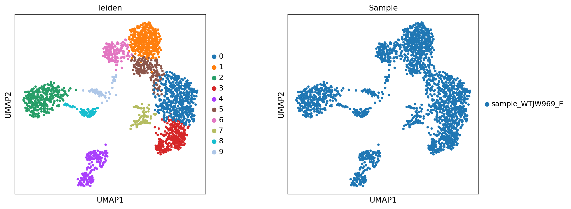

Figure Legend: This figure shows the expression distribution of specific marker genes in the UMAP dimensionality reduction space of RNA data.

• X and Y axes: The two main dimensions after UMAP reduction (UMAP1 and UMAP2).
• Color: Color depth indicates expression levels of marker genes; darker means higher expression. Markers shown include: CD3D, THEMIS (T cells), NKG7 (NK cells), CD8A (CD8+ T cells), CD4 (CD4+ T cells), CD79A and MS4A1 (B cells), JCHAIN (Plasma cells), LYZ (Monocytes), LILRA4 (pDC cells).
• Dots: Each dot represents an individual cell.
• Purpose: Through marker gene expression patterns, different cell types can be preliminarily identified and validated to assist in cell type annotation.

colors = ["#F5E6CC", "#FDBB84", "#E34A33", "#7F0000"]
my_warm_cmap = mcolors.LinearSegmentedColormap.from_list("white_orange_red", colors, N=256)

marker_names = ["CD3D", "THEMIS", "NKG7", "CD8A", "CD4", "IL7R", "S100A4", "CCR7",
                "CD79A","MS4A1","JCHAIN",
                "LYZ","FCN1","FCGR3A","CST3","MKI67"]
sc.pl.umap(
    adata_rna, 
    color=marker_names, 
    ncols=4,            
    color_map=my_warm_cmap, 
    vmax='p99',         
    s=10,               
    frameon=False,      
    vmin=0,
    show=False 
)

plt.gcf().set_size_inches(12, 8) 
plt.show()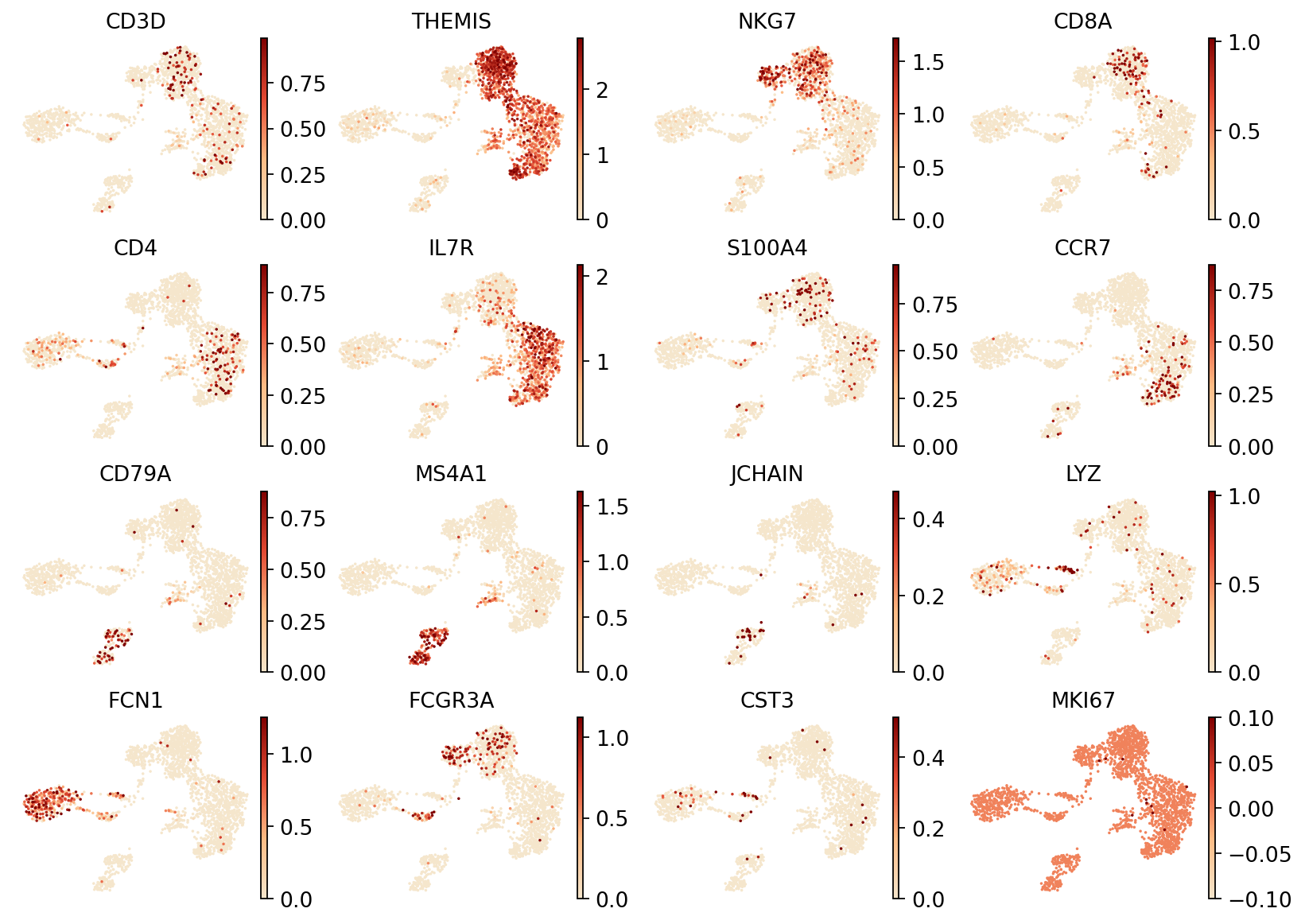

celltype = {
    '0': 'Navie CD4+ T',
    '1': 'CD8+ T',
    '2': 'CD14+ Mono',
    '3': 'Memory CD4+ T',
    '4': 'B',
    '5': 'T',
    '6': 'NK',
    '7': 'Multiplet',
    '8': 'FCGR3A+ Mono',
    '9': 'DC'
    
    
}
adata_rna.obs['celltype'] = adata_rna.obs['leiden'].map(celltype)

if not 'celltype' in adata_rna.obs.columns:
   adata_rna.obs['celltype'] = adata_rna.obs['leiden']

Figure Legend: This figure shows the UMAP plot of cell type based on transcriptome data.

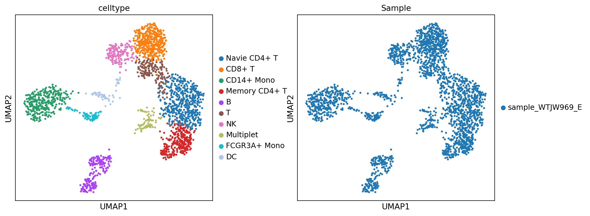
• Left Panel: Each dot represents a cell, and colors represent different cell type (celltype).
• Right Panel: Each dot represents a cell, and colors represent different samples (Sample).

sc.set_figure_params(scanpy=True, fontsize=12, facecolor='white', figsize=(5, 5), dpi = 80)
sc.pl.umap(
    adata_rna, 
    color=['celltype', 'Sample'], 
    ncols=2,
    s=35,
    wspace=0.3
)

Build MuData Object and Train MOFA+ Model

os.makedirs(f"{outdir}/models", exist_ok=True)

mu_list = {}
mu_list['rna'] = adata_rna
for i in adata_met_list.keys():
    mu_list[f'methy_{i}'] =  adata_met_list[i]
mu_list

output

{'rna': AnnData object with n_obs × n_vars = 2189 × 38606
obs: 'orig.ident', 'nCount_RNA', 'nFeature_RNA', 'mito', 'Sample', 'raw_Sample', 'resolution.0.5_d30', 'CellAnnotation', 'original_barcode', 'chemistry', 'n_genes_by_counts', 'log1p_n_genes_by_counts', 'total_counts', 'log1p_total_counts', 'pct_counts_in_top_50_genes', 'pct_counts_in_top_100_genes', 'pct_counts_in_top_200_genes', 'pct_counts_in_top_500_genes', 'total_counts_mt', 'log1p_total_counts_mt', 'pct_counts_mt', 'total_counts_ribo', 'log1p_total_counts_ribo', 'pct_counts_ribo', 'total_counts_hb', 'log1p_total_counts_hb', 'pct_counts_hb', 'leiden', 'celltype'
var: 'gene_ids', 'feature_types', 'mt', 'ribo', 'hb', 'n_cells_by_counts', 'mean_counts', 'log1p_mean_counts', 'pct_dropout_by_counts', 'total_counts', 'log1p_total_counts', 'highly_variable', 'highly_variable_rank', 'means', 'variances', 'variances_norm', 'highly_variable_nbatches'
uns: 'log1p', 'hvg', 'pca', 'neighbors', 'umap', 'tsne', 'leiden', 'leiden_colors', 'Sample_colors', 'celltype_colors'
obsm: 'X_pca', 'X_umap', 'X_tsne'
varm: 'PCs'
layers: 'counts'
obsp: 'distances', 'connectivities',
'methy_geneslop2k': AnnData object with n_obs × n_vars = 2189 × 25405
obs: 'total_cpg_number', 'genome_cov', 'reads_counts', 'CpG%', 'CH%', 'Sample', 'original_barcode', 'chemistry'
var: 'chrom', 'end', 'start', 'cov_mean', 'mean', 'dispersion', 'cov', 'score', 'feature_select', 'highly_variable'}

Build Multi-modal Container (MuData) and Model Training

MuData is a data structure designed specifically for multi-omics data, capable of storing and managing data from multiple modalities (e.g., RNA, Methylation) and their associations simultaneously.

MOFA+ Model Training Parameters Description:

• groups_label: Used for multi-sample/multi-batch analysis, the model will attempt to correct batch effects.
• n_factors: Expected number of latent factors to discover (default 10). More factors can capture more details but increase computational load and may introduce noise.
• scale_views: Whether to scale each modality. Default is False to balance data scale differences between modalities.
• convergence_mode: Convergence mode, with slow, medium, and fast options. slow mode trains more thoroughly for more stable results; fast mode is quicker.

# Build a MuData object to integrate RNA and methylation data
mdata = mu.MuData(mu_list)
mdata.obs['Sample'] = mdata['rna'].obs['Sample']
mdata.obs['celltype'] = mdata['rna'].obs['celltype']
mdata.obs['CpG%'] = mdata[mdata.mod_names[1]].obs['CpG%']
mdata

MuData object with n_obs × n_vars = 2189 × 64011
  obs:	'Sample', 'celltype', 'CpG%'
  var:	'highly_variable'
  2 modalities
    rna:	2189 x 38606
      obs:	'orig.ident', 'nCount_RNA', 'nFeature_RNA', 'mito', 'Sample', 'raw_Sample', 'resolution.0.5_d30', 'CellAnnotation', 'original_barcode', 'chemistry', 'n_genes_by_counts', 'log1p_n_genes_by_counts', 'total_counts', 'log1p_total_counts', 'pct_counts_in_top_50_genes', 'pct_counts_in_top_100_genes', 'pct_counts_in_top_200_genes', 'pct_counts_in_top_500_genes', 'total_counts_mt', 'log1p_total_counts_mt', 'pct_counts_mt', 'total_counts_ribo', 'log1p_total_counts_ribo', 'pct_counts_ribo', 'total_counts_hb', 'log1p_total_counts_hb', 'pct_counts_hb', 'leiden', 'celltype'
      var:	'gene_ids', 'feature_types', 'mt', 'ribo', 'hb', 'n_cells_by_counts', 'mean_counts', 'log1p_mean_counts', 'pct_dropout_by_counts', 'total_counts', 'log1p_total_counts', 'highly_variable', 'highly_variable_rank', 'means', 'variances', 'variances_norm', 'highly_variable_nbatches'
      uns:	'log1p', 'hvg', 'pca', 'neighbors', 'umap', 'tsne', 'leiden', 'leiden_colors', 'Sample_colors', 'celltype_colors'
      obsm:	'X_pca', 'X_umap', 'X_tsne'
      varm:	'PCs'
      layers:	'counts'
      obsp:	'distances', 'connectivities'
    methy_geneslop2k:	2189 x 25405
      obs:	'total_cpg_number', 'genome_cov', 'reads_counts', 'CpG%', 'CH%', 'Sample', 'original_barcode', 'chemistry'
      var:	'chrom', 'end', 'start', 'cov_mean', 'mean', 'dispersion', 'cov', 'score', 'feature_select', 'highly_variable'

# Intersect cells across modalities to ensure one-to-one correspondence
mu.pp.intersect_obs(mdata)

# Run the MOFA+ model
mu.tl.mofa(mdata,
           use_raw = False,
           groups_label = 'Sample', # Sample grouping column for handling batch effects
           scale_views=True,        # Balance weights across modalities
           n_factors=10,            # Number of latent factors
           convergence_mode='slow', # Use slow mode for more robust convergence
           use_var = 'highly_variable', # Train using highly variable features only
           outfile=f"{outdir}/models/pbmc_969_multi_methy.hdf5") # Model output path

        #########################################################
        ###           __  __  ____  ______                    ### 
        ###          |  \/  |/ __ \|  ____/\    _             ### 
        ###          | \  / | |  | | |__ /  \ _| |_           ### 
        ###          | |\/| | |  | |  __/ /\ \_   _|          ###
        ###          | |  | | |__| | | / ____ \|_|            ###
        ###          |_|  |_|\____/|_|/_/    \_\              ###
        ###                                                   ### 
        ######################################################### 
       
 
        
Scaling views to unit variance...

Loaded view='rna' group='sample_WTJW969_E' with N=2189 samples and D=2000 features...
Loaded view='methy_geneslop2k' group='sample_WTJW969_E' with N=2189 samples and D=2500 features...


Model options:
- Automatic Relevance Determination prior on the factors: True
- Automatic Relevance Determination prior on the weights: True
- Spike-and-slab prior on the factors: False
- Spike-and-slab prior on the weights: True
Likelihoods:
- View 0 (rna): gaussian
- View 1 (methy_geneslop2k): gaussian




######################################
## Training the model with seed 1 ##
######################################



Converged!



#######################
## Training finished ##
#######################


Warning: Output file /home/weiqiuxia/workspace/project/weiqiuxia/MOFA_results/models/pbmc_969_multi_methy.hdf5 already exists, it will be replaced
Saving model in /home/weiqiuxia/workspace/project/weiqiuxia/MOFA_results/models/pbmc_969_multi_methy.hdf5...
Saved MOFA embeddings in .obsm['X_mofa'] slot and their loadings in .varm['LFs'].

mdata.uns = mdata.uns or dict()

MOFA Factor Visualization

One of the core results of MOFA+ factor analysis is the inferred latent factors. We can visualize the distribution of these factors in cells to understand biological differences between different cell types.

Figure Legend: This figure (scatter plot matrix) shows the distribution of the first 10 MOFA factors (pairwise) in cells.

• Color: Represents cell type (rna:celltype) or methylation level (methy_geneslop2k:CpG%).
• Observation: If a factor (e.g., Factor 1) can clearly separate a certain cell type (e.g., B cells) from other cells, it indicates that this factor captures specific biological signals of that cell type.

mu.pl.mofa(mdata, color="celltype", components=["1,2", "3,4", "5,6", "7,8", "9,10"])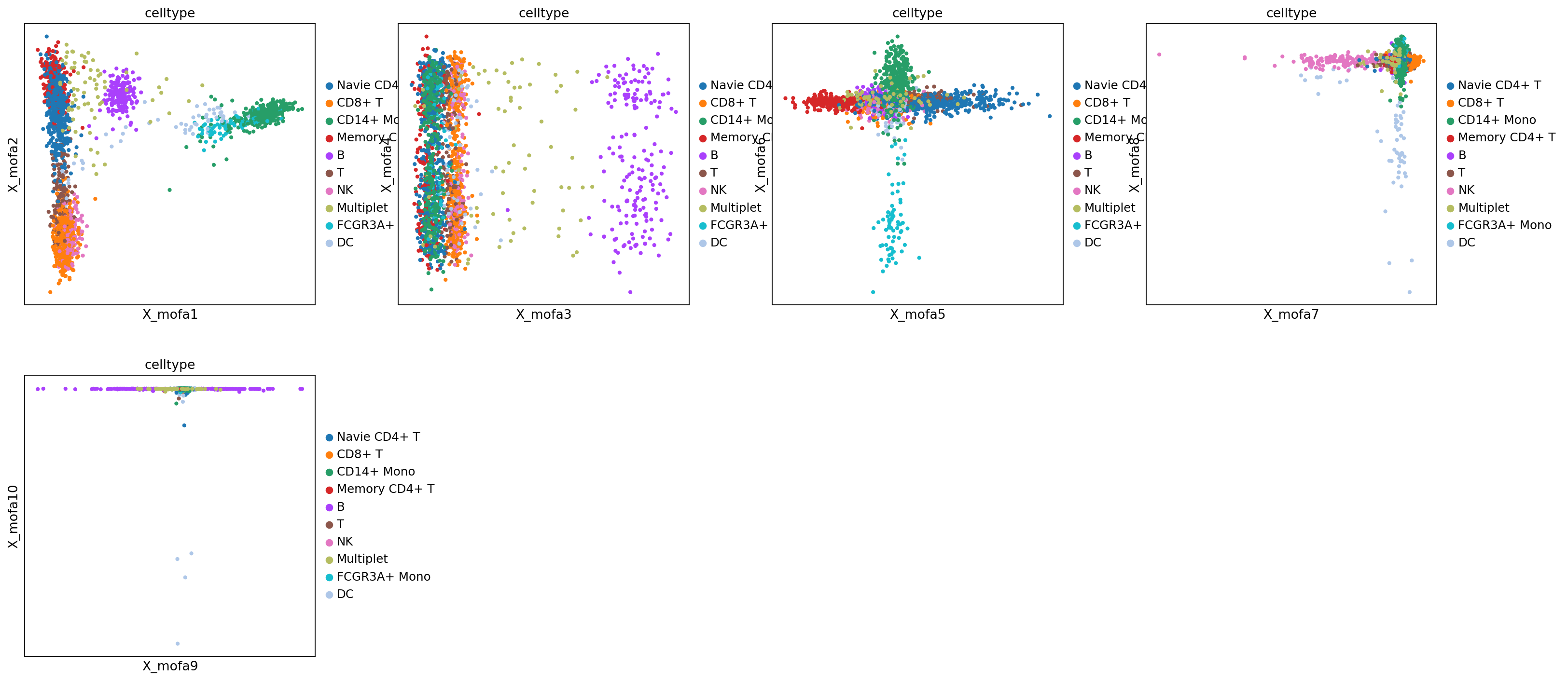

mu.pl.mofa(mdata, color="CpG%", components=["1,2", "3,4", "5,6", "7,8","9,10"])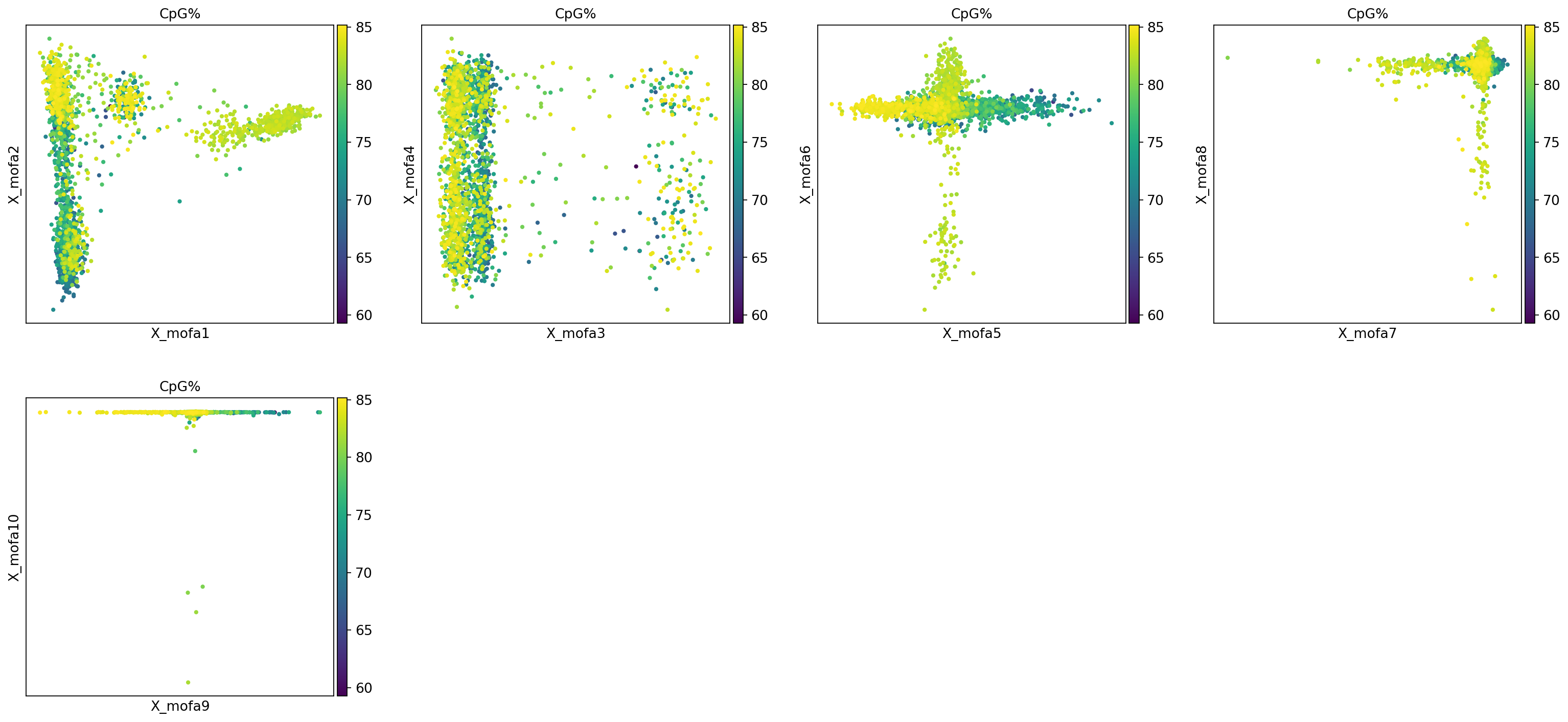

Model Evaluation and Variance Explanation (R2)

Assess the explanation degree (Variance Explained, R2) of each factor for the variation of different omics modalities.

model = mfx.mofa_model(f"{outdir}/models/pbmc_969_multi_methy.hdf5")
model

output

MOFA+ model: pbmc 969 multi methy
Samples (cells): 2189
Features: 4500
Groups: sample_WTJW969_E (2189)
Views: methy_geneslop2k (2500), rna (2000)
Factors: 10
Expectations: W, Z

model.get_r2()

	Factor	View	Group	R2
0	Factor1	rna	sample_WTJW969_E	1.755070e+01
1	Factor1	methy_geneslop2k	sample_WTJW969_E	1.526547e-06
2	Factor2	rna	sample_WTJW969_E	6.230776e+00
3	Factor2	methy_geneslop2k	sample_WTJW969_E	1.247076e-05
4	Factor3	rna	sample_WTJW969_E	5.786080e+00
5	Factor3	methy_geneslop2k	sample_WTJW969_E	6.985795e-07
6	Factor4	rna	sample_WTJW969_E	5.757473e-06
7	Factor4	methy_geneslop2k	sample_WTJW969_E	2.565718e+00
8	Factor5	rna	sample_WTJW969_E	1.429741e+00
9	Factor5	methy_geneslop2k	sample_WTJW969_E	1.103752e-04
10	Factor6	rna	sample_WTJW969_E	9.622432e-01
11	Factor6	methy_geneslop2k	sample_WTJW969_E	7.399176e-06
12	Factor7	rna	sample_WTJW969_E	8.270760e-01
13	Factor7	methy_geneslop2k	sample_WTJW969_E	2.246223e-06
14	Factor8	rna	sample_WTJW969_E	5.685163e-01
15	Factor8	methy_geneslop2k	sample_WTJW969_E	3.142382e-06
16	Factor9	rna	sample_WTJW969_E	4.485491e-01
17	Factor9	methy_geneslop2k	sample_WTJW969_E	2.246235e-05
18	Factor10	rna	sample_WTJW969_E	8.303199e-02
19	Factor10	methy_geneslop2k	sample_WTJW969_E	-2.510329e-07

r2_df = model.get_r2()
r2_df[r2_df['R2'] >= 1]

	Factor	View	Group	R2
0	Factor1	rna	sample_WTJW969_E	17.550695
2	Factor2	rna	sample_WTJW969_E	6.230776
4	Factor3	rna	sample_WTJW969_E	5.786080
7	Factor4	methy_geneslop2k	sample_WTJW969_E	2.565718
8	Factor5	rna	sample_WTJW969_E	1.429741

Figure Legend: This heatmap shows the explanatory power of each MOFA factor (Factor) for the variation of different omics modalities (View).

• X-axis: MOFA Factors (Factor 1, 2, ...).
• Y-axis: Omics Modalities (RNA, Methylation).
• Color Intensity: R2 value (Variance Explained), darker color indicates greater contribution of the factor to that modality.
• Significance: If a factor is dark in both modalities, it is usually a Shared Factor; if dark in only one modality, it is usually a Private Factor.

mfx.plot_r2(model, x='View', vmax=10)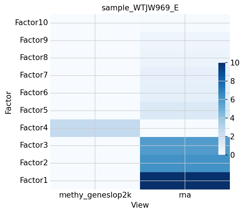

model.close()

Downstream Analysis Based on MOFA Factors

Use MOFA extracted latent factors (X_mofa) to replace original features, construct a neighbor graph, and perform UMAP dimensionality reduction and Leiden clustering. Combine with transcriptome annotation results to assess if a clearer cell atlas can be obtained.

In this step, we typically select factors with high variance explanation for subsequent analysis.

sc.pp.neighbors(mdata, use_rep="X_mofa", n_pcs=5, random_state=20)
sc.tl.umap(mdata, min_dist=.2, spread=1., random_state=20)
sc.tl.leiden(mdata, resolution=.5, random_state=20)

Figure Legend: This figure shows the UMAP dimensionality reduction plot constructed based on MOFA factors.

• This figure integrates information from RNA and Methylation, usually distinguishing cell subpopulations better than single-modality clustering.
• Color Legend:
  • celltype: Cell type annotation based on transcriptome data.
  • leiden: Clustering results based on MOFA factors.
  • CpG%: Genome-wide CpG methylation level.
  • Sample: Sample source.

sc.pl.umap(mdata, color=["celltype","leiden",'CpG%', 'Sample'],legend_loc="on data", legend_fontoutline=1)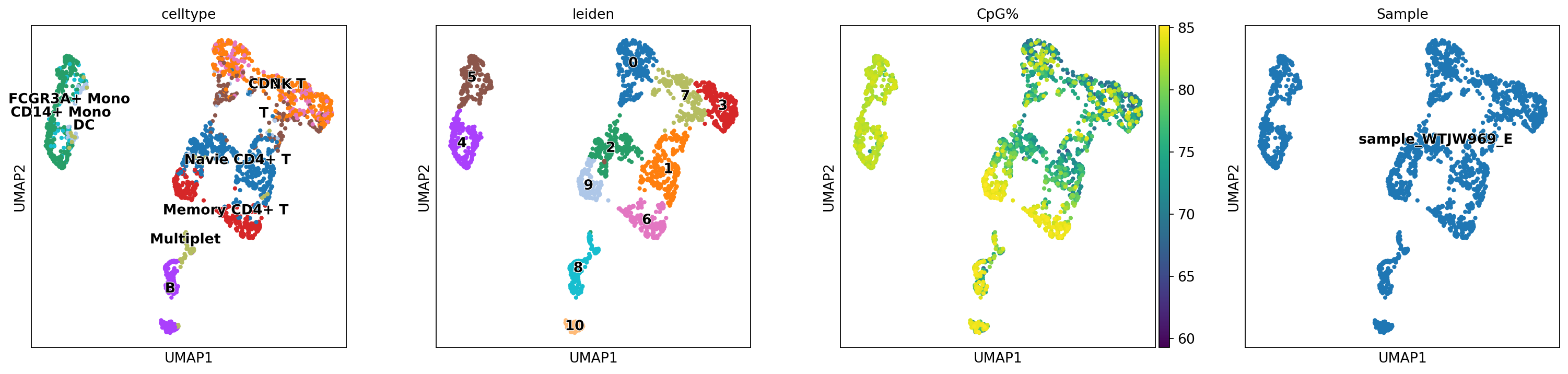

Results Discussion and Optimization Suggestions

MOFA+ performs subsequent multi-modal integration analysis based on highly variable features, so it is significantly affected by the selected High Variable Feature Set. If the selected high variable feature set itself cannot correctly distinguish different biological cell groups, the integration result of MOFA+ will also be limited.

As shown in the figure above, if the multi-modal integration clustering effect of MOFA+ is not as good as the single-omics (e.g., RNA only) clustering result, a possible reason is that the methylation region granularity we used is "too large" (e.g., geneslop2k refers to the gene region plus its upstream and downstream 2kb). Existing literature indicates that methylation levels in different gene regions (such as promoters, enhancers, gene bodies) have different regulatory meanings. Coarse-grained regions may mask fine biological signals, leading to the selected high variable feature set containing more noise, thereby affecting the integration effect of MOFA+.

Optimization Strategy: Successful cases of integrating methylation and transcriptome data using MOFA+ indicate that precise screening of methylation feature sets is crucial. For example, in the literature Multi-omics profiling of mouse gastrulation at single-cell resolution, researchers adopted the following strategy:

1. Feature Pre-screening: Use public data or ChIP-seq data to first locate key regulatory regions related to sample types, such as H3K27ac (Enhancers), H3K4me3 (TSS), and 2kb regions upstream and downstream of protein-coding gene transcription start sites (Promoters).
2. High Variable Screening: Perform high variable feature screening based on these selected regions.
3. Factor Discovery: Identify factors strongly related to biological processes in the methylation modality.

By this method, the signal-to-noise ratio of input features can be significantly improved, thereby enhancing the effect of MOFA+ integration analysis.

Output Files and Subsequent Reuse

After analysis is complete, we write three objects to outdir:

• adata_rna.h5ad: RNA AnnData object.
• adata_met_**.h5ad: Methylation AnnData object.
• mdata.h5mu: Multi-omics MuData object.

Note:

• .h5mu files are usually large, it is recommended to keep them in a stable path and back them up.
• If you change filtering thresholds or var_dim parameters, it is recommended to rerun the full workflow and overwrite output files.

adata_rna.write_h5ad(f'{outdir}/adata_rna.h5ad')
for i in adata_met_list.keys():
    adata_met_list[i].write_h5ad(f'{outdir}/adata_met_{i}.h5ad')
mdata.write(f'{outdir}/mdata.h5mu')

More Resources

• Muon Official Tutorial: For other analysis tutorials on integrating multi-modal data with MOFA+, please see the Muon Website.
• MOFA+ Downstream Analysis: For downstream analysis after MOFA+ (such as factor annotation, gene set enrichment, etc.), please see the mofax tutorial.