scMethyl + RNA Multi-omics: Integration Tutorial Using WNN

Author: SeekGene

Time: 31 min

Words: 6.2k words

Updated: 2026-03-30

Reads: 0 times

scMethyl + RNA-seq Notebooks

Module Introduction

This tutorial explains how to integrate single-cell DNA methylation and transcriptome (RNA) data using the Scanpy and Muon frameworks. You will build a joint embedding, perform clustering, and visualize results in a unified UMAP space.

WNN Principles

WNN (Weighted Nearest Neighbors) is an unsupervised approach that integrates multiple modalities by learning how much each modality should contribute for each cell.

• Build modality-specific neighbor graphs: compute k-nearest neighbors (kNN) for RNA in PCA space, and for methylation in LSI space.
• Estimate cell-specific modality weights: compare local neighborhood consistency across modalities; the modality that better captures a cell’s local structure receives a higher weight for that cell.
• Fuse into a WNN graph for downstream analysis: combine the modality graphs using the learned weights, then run UMAP and Leiden clustering on the fused graph.

Analysis Objectives

• Joint clustering: integrate complementary signals from both modalities to separate cell populations more robustly.
• Modality contribution: assess how much RNA vs methylation contributes to similarity for each cell.
• Unified visualization: display an integrated cell atlas in a single UMAP space.

Input File Preparation

Before you start, prepare matched methylation and RNA data from the same set of cells:

• Methylation data: MCDS format (usually generated by the ALLCools pipeline).
• RNA data: a .rds or .qs file (used to export an expression matrix and load it in Scanpy).
• Barcode mapping table: for DD-MET3, use DD-M_bUCB3_whitelist.csv to align barcodes across modalities.

import os
import re
import glob
import warnings
import numpy as np
import pandas as pd
import xarray as xr
import matplotlib.pyplot as plt
import matplotlib.colors as mcolors
from matplotlib.lines import Line2D
from scipy import sparse

# Bioinformatics core libraries
import scanpy as sc
import scanpy.external as sce
import muon as mu
from muon import atac as ac
from ALLCools.mcds import MCDS
from ALLCools.clustering import (
    tsne, significant_pc_test, log_scale, lsi, binarize_matrix, 
    filter_regions, cluster_enriched_features, ConsensusClustering, 
    Dendrogram, get_pc_centers, one_vs_rest_dmg
)
from ALLCools.clustering.doublets import MethylScrublet
from ALLCools.plot import *
from harmonypy import run_harmony
from skmisc.loess import loess

# Configure R environment (for calling R packages via rpy2)
r_base_path = '/PROJ/home/weiqiuxia/micromamba/envs/muon_env'
os.environ['R_HOME'] = os.path.join(r_base_path, 'lib', 'R') 
os.environ['LD_LIBRARY_PATH'] = os.path.join(r_base_path, 'lib', 'R', 'lib') + ':' + os.environ.get('LD_LIBRARY_PATH', '')
r_lib_path = os.path.join(r_base_path, 'lib', 'R', 'library')
os.environ['R_LIBS'] = r_lib_path
os.environ['R_LIBS_USER'] = r_lib_path
os.environ['R_LIBS_SITE'] = r_lib_path

# Global settings
sc.settings.verbosity = 0
warnings.filterwarnings('ignore')
sc.set_figure_params(dpi=80, figsize=(5, 5))
plt.rcParams['figure.dpi'] = 80  
plt.rcParams['savefig.dpi'] = 300      
plt.rcParams['figure.figsize'] = (5, 5)

try:
    from matplotlib_venn import venn2
    HAS_VENN = True
except Exception:
    HAS_VENN = False

def mcds_to_adata(mcds_path, var_dim='chrom20k', mc_type='CGN', quant_type='hypo-score'):
    """
    Convert xarray format hypo-score matrix to AnnData object.
    
    Parameters:
    mcds_path: MCDS file path
    var_dim: Variable dimension, e.g., 'chrom20k'
    mc_type: Methylation type, e.g., 'CGN'
    quant_type: Quantification type, e.g., 'hypo-score'
    """
    mcds = MCDS.open(mcds_path, obs_dim='cell', var_dim=var_dim)
    adata = mcds.get_score_adata(mc_type=mc_type, quant_type=quant_type, sparse=True)
    return adata

def compute_cg_ch_level(df):
    """
    Calculate CpG and CH methylation levels.
    
    Parameters:
    df: DataFrame containing mc and cov columns
    """
    cg_cov_col = [i for i in df.columns[df.columns.str.startswith('CG')].to_list() if i.endswith('_cov')]
    cg_mc_col = [i for i in df.columns[df.columns.str.startswith('CG')].to_list() if i.endswith('_mc')]
    ch_cov_col = [i for i in df.columns[df.columns.str.contains('^(CT|CC|CA)')].to_list() if i.endswith('_cov')]
    ch_mc_col = [i for i in df.columns[df.columns.str.contains('^(CT|CC|CA)')].to_list() if i.endswith('_mc')]
    
    df['CpG_cov'] = df[cg_cov_col].sum(axis=1)
    df['CpG_mc'] = df[cg_mc_col].sum(axis=1)
    df['CpG%'] = round(df['CpG_mc'] * 100 / df['CpG_cov'], 2)
    
    df['CH_cov'] = df[ch_cov_col].sum(axis=1)
    df['CH_mc'] = df[ch_mc_col].sum(axis=1)
    df['CH%'] = round(df['CH_mc'] * 100 / df['CH_cov'], 2)

    return df

def check_barcode_overlap(rna_adata, met_adata, barcode_map=None):
    """
    检查转录组和Methylation Data的细胞 Barcode 重叠情况，并根据共同 Barcode 进行子集提取。
    Handle DD-MET3 and DD-MET5 technologies respectively.
    """
    # Extract original Barcodes
    rna_adata.obs['original_barcode'] = [re.sub('_.*', '', i) for i in rna_adata.obs.index]
    met_adata.obs['original_barcode'] = [re.sub('_.*', '', i) for i in met_adata.obs.index]
    
    # Calculate initial overlap rate
    overlap_rate = len(set(rna_adata.obs['original_barcode']) & set(met_adata.obs['original_barcode'])) / met_adata.shape[0]
    
    if overlap_rate < 0.1:
        # Handle DD-MET3 case: Need to convert Barcodes using mapping table
        met2rna_barcode = barcode_map[barcode_map['m_cb'].isin(met_adata.obs['original_barcode'])]
        rna_adata = rna_adata[rna_adata.obs['original_barcode'].obs.index.isin(met2rna_barcode['gex_cb'])]
        met2rna_barcode = met2rna_barcode.set_index('gex_cb')
        rna_adata.obs['gex_cb'] = rna_adata.obs.index
        rna_adata.obs.index = met2rna_barcode.loc[rna_adata.obs['original_barcode'], 'm_cb']
        
        overlap_rate_test = len(set(rna_adata.obs.index) & set(met_adata.obs.index)) / met_adata.shape[0]
        chemistry = 'DD-MET3'
        if overlap_rate_test < 0.1:
            raise Exception('转录组与Methylation Data的 Barcode 重叠率低于 10%，请检查输入数据。')
    else:
        # Handle DD-MET5 case: Barcodes correspond directly
        chemistry = 'DD-MET5'
        rna_adata.obs.index = rna_adata.obs['original_barcode']
        met_adata.obs.index = met_adata.obs['original_barcode']
        
    # Extract common cells and synchronize both objects
    common_index = list(set(rna_adata.obs.index) & set(met_adata.obs.index))
    rna_adata = rna_adata[rna_adata.obs.index.isin(common_index)]
    rna_adata.obs['chemistry'] = chemistry
    met_adata = met_adata[met_adata.obs.index.isin(common_index)]
    met_adata.obs['chemistry'] = chemistry
    
    return rna_adata, met_adata, chemistry

def parse_gtf(gtf_file, output_file):
    """
    Parse GTF file and extract gene type information.
    """
    with open(gtf_file, 'r') as f_in, open(output_file, 'w') as f_out:
        for line in f_in:
            if line.startswith('#'):
                continue
            parts = line.strip().split('\t')
            if len(parts) < 9:
                continue
            
            feature_type = parts[2]
            if feature_type != 'gene':
                continue
            
            attributes = parts[8]
            attr_dict = {}
            for attr in attributes.split(';'):
                attr = attr.strip()
                if not attr:
                    continue
                if ' ' in attr:
                    key, value = attr.split(' ', 1)
                    value = value.strip('"')
                    attr_dict[key] = value
            
            gene_id = attr_dict.get('gene_id', '')
            gene_name = attr_dict.get('gene_name', '')
            gene_type = attr_dict.get('gene_type', '')
            
            col1 = f"{gene_id}_{gene_name}" if gene_id and gene_name else (gene_id or gene_name)
            f_out.write(f"{col1}\t{gene_type}\n")

def rds_to_matrix(filepath, outdir):
    """
    Call R script to convert Seurat object (.rds or .qs) to 10X standard matrix format.
    """
    import rpy2.robjects as robjects
    robjects.globalenv['rdsfile'] = filepath
    robjects.globalenv['outdir'] = outdir
    
    # Execute R code
    robjects.r('''
    library(Seurat)
    library(qs)
    
    if(endsWith(rdsfile, ".rds")){
        obj <- readRDS(rdsfile)
    } else {
        obj <- qread(rdsfile)
    }
    
    dir.create(outdir, recursive = TRUE, showWarnings = FALSE)

    # Export Counts matrix
    Matrix::writeMM(GetAssayData(obj, assay = "RNA", layer = "counts"), file = file.path(outdir, "matrix.mtx"))
    system(paste0("gzip -f ", file.path(outdir, "matrix.mtx")))
    
    # Export Features information
    features <- data.frame(Feature_id = rownames(obj), Feature_name = rownames(obj), Feature_type = "Gene Expression")
    write.table(features, file.path(outdir, "features.tsv"), row.names = F, col.names = F, sep = "\t", quote = F)
    system(paste0("gzip -f ", file.path(outdir, "features.tsv")))
    
    # Export Barcodes information
    barcodes <- data.frame(Barcode = colnames(obj))
    write.table(barcodes, file.path(outdir, "barcodes.tsv"), row.names = F, col.names = F, sep = "\t", quote = F)
    system(paste0("gzip -f ", file.path(outdir, "barcodes.tsv")))

    # Export metadata
    meta <- obj@meta.data
    write.table(tibble::rownames_to_column(meta, "barcode"), file.path(outdir, "meta.csv"), row.names = FALSE, col.names = TRUE, sep = ",", quote = F)
    ''')

output

/PROJ/home/weiqiuxia/micromamba/envs/muon_env/lib/python3.12/site-packages/numcodecs/__init__.py:106: DeprecationWarning: crc32c usage is deprecated since numcodecs v0.16.4. It is recommended to install google_crc32c instead.
from numcodecs.checksum32 import CRC32, Adler32, JenkinsLookup3
/PROJ/home/weiqiuxia/micromamba/envs/muon_env/lib/python3.12/site-packages/tqdm/auto.py:21: TqdmWarning: IProgress not found. Please update jupyter and ipywidgets. See https://ipywidgets.readthedocs.io/en/stable/user_install.html
from .autonotebook import tqdm as notebook_tqdm
/PROJ/home/weiqiuxia/micromamba/envs/muon_env/lib/python3.12/site-packages/muon/_core/preproc.py:31: FutureWarning: \`__version__\` is deprecated, use \`importlib.metadata.version('scanpy')\` instead
if Version(scanpy.__version__) < Version("1.10"):

Parameter Settings

Input Directory Structure Description

Important: This workflow requires a specific input directory structure. The program will automatically retrieve RNA- and methylation-related input files based on indir. We recommend organizing your data like this:

data/AY1768874914782/ (indir)
├── input.rds                                          # Transcriptome data (Seurat object or qs format)
└── methylation                                        # Methylation data root directory
    └── demoWTJW969-task-1                             # Task/Batch name
        └── WTJW969                                    # Sample name
            ├── allcools_generate_datasets
            │   └── WTJW969.mcds                       # MCDS dataset folder
            │       ├── chrom20k                       # Methylation score matrix for 20 kb windows
            │       └── ...
            └── split_bams
                ├── filtered_barcode_reads_counts.csv  # Filtered barcode-level mapped-read counts
                └── WTJW969_cells.csv                  # Filtered cell QC metrics (CpG count, coverage, etc.)

• RNA data: match .rds or .qs files under indir.
• Methylation data: retrieve MCDS files and associated QC CSV files under indir/methylation.

# --------------------------
# 1. Path and Sample Settings
# --------------------------

# indir: Input data directory
# Note: This directory should contain transcriptome files (.rds/.qs) and a methylation folder
# If there are multiple batches of data in different directories, you can separate multiple paths with commas, e.g., '/path/to/data1,/path/to/data2'
indir = '/home/weiqiuxia/workspace/data/AY1768874914782/'

# outdir: Output directory for analysis results
# All generated intermediate files and final results will be saved in this directory
outdir = '/home/weiqiuxia/workspace/project/weiqiuxia/WNN_results'

# sample_col: Sample column name
# Used to distinguish different samples in metadata, default 'Sample'. It must match the sample folder name under the `indir/methylation` path
sample_col = 'Sample'

# --------------------------
# 2. Methylation Analysis Parameters
# --------------------------

# var_dim: Methylation feature dimension
# 'chrom20k' means dividing the genome into 20kb windows for analysis, which is a common granularity for single-cell methylation
var_dim = 'chrom20k'

# total_cpg_number_cutoff: CpG coverage threshold
# Filter out low-quality cells with a total number of detected CpG sites less than this value
total_cpg_number_cutoff = 500

# dd_met3_barcode_map：DD-MET3 技术专用的 Barcode Mapping Table
# If DD-MET3 library prep technology is used, the Barcode sequences of transcriptome and methylation are not exactly the same, and this table is required for conversion
dd_met3_barcode_map = '/home/weiqiuxia/workspace/project/weiqiuxia/DD-M_bUCB3_whitelist.csv'

# resolution: Clustering resolution
# Controls the fineness of clustering; larger values yield more cell subpopulations
resolution = 1

# --------------------------
# 3. RNA Analysis Parameters (Optional)
# --------------------------

# rna_meta: External RNA metadata file path (optional)
# If additional cell annotation information needs to be imported, specify the CSV file path here
rna_meta = None

# anno_col: Cell annotation column name
# Specify the column name in RNA metadata used to label cell types
anno_col = 'CellAnnotation'

# reduction_col_prefix: Dimensionality reduction coordinate column prefix (optional)
# If RNA metadata already contains UMAP or t-SNE coordinates (e.g., 'UMAP_1', 'UMAP_2'), you can specify the prefix here
reduction_col_prefix = ''

# Automatically create output directory
os.makedirs(outdir, exist_ok=True)

Data Loading

This step loads RNA and methylation data separately, then matches cells across modalities using barcodes.

Main workflow:

1. Load the barcode mapping table (DD-MET3 only): convert barcodes so both modalities can be aligned.
2. Convert and load RNA data: detect .qs or .rds, export to Matrix Market format, then load with Scanpy.
3. Load methylation data and merge metadata: traverse directories to read MCDS and QC tables, then intersect with RNA cells by barcode.

# 读取 DD-MET3 Barcode Mapping Table
# This table is used to solve the problem of inconsistent Barcodes in RNA and Methylation data
if os.path.exists(dd_met3_barcode_map):
    dd_met3_barcode_map_df = pd.read_csv(dd_met3_barcode_map, header=0)
else:
    print(f"Warning: Barcode map file not found at {dd_met3_barcode_map}. This is only required for DD-MET3 data.")
    dd_met3_barcode_map_df = None

# First, obtain files ending in qs or rds, convert them to matrix files, and then read with scanpy
for i in os.listdir(indir):
    if i.endswith('.qs'):
        rds_to_matrix(os.path.join(indir, i), os.path.join(outdir, 'input_matrix'))
        break

output

R callback write-console: Loading required package: SeuratObject

R callback write-console: Loading required package: sp

R callback write-console:
Attaching package: ‘SeuratObject’


R callback write-console: The following objects are masked from ‘package:base’:

intersect, t


R callback write-console: qs 0.27.3. Announcement: https://github.com/qsbase/qs/issues/103

# Scanpy reads RNA data
adata_rna = sc.read_10x_mtx(f'{outdir}/input_matrix/')
meta = pd.read_csv(f'{outdir}/input_matrix/meta.csv', index_col = 0, header = 0)
adata_rna.obs = meta
adata_rna.obs['CellAnnotation'] = adata_rna.obs['CellAnnotation'].astype('category')

#Read Methylation Data, then intersect with transcriptome data to ensure cells and barcodes are consistent between methylation and transcriptome data
keep_col = ['barcode', 'total_cpg_number', 'genome_cov', 'reads_counts', 'CpG%', 'CH%']
obj_met_list = {}
obj_rna_list = {}
indirs = indir.split(',')
samples = []
mcds_paths = {}
sample_path = {}
analysis_batch_dir = os.listdir(os.path.join(indir, 'methylation'))
for i in analysis_batch_dir:
    if os.path.isdir(os.path.join(indir, 'methylation', i)):
        a_batch_dir = os.path.join(indir, 'methylation', i)
        # Get all samples under the analysis batch
        samples.extend([ i for i in os.listdir(a_batch_dir)])
        for s in samples:
            mcds_path = os.path.join(a_batch_dir, f'{s}','allcools_generate_datasets', f'{s}.mcds')
            mcds_paths[s] = mcds_path 
            sample_path[s] = a_batch_dir        
            obj = mcds_to_adata(mcds_path, var_dim = var_dim)
            obj_met_list[s] = obj
            
            # Read methylation-related QC results
            s_cells_meta = pd.read_csv(os.path.join(a_batch_dir, s, 'split_bams', f'{s}_cells.csv'), header = 0)
            s_cells_meta['barcode'] = [b.replace('_allc.gz','') for b in s_cells_meta['cell_barcode']]
            # Read mapped reads for each cell
            s_reads_counts = pd.read_csv(os.path.join(a_batch_dir, s, 'split_bams', 'filtered_barcode_reads_counts.csv'), header = 0)
            s_merged_df = s_cells_meta.merge(s_reads_counts, how = 'inner', left_on = 'barcode', right_on = 'barcode')
            # Merge the above two dataframes
            s_merged_df = compute_cg_ch_level(s_merged_df)
            s_merged_df = s_merged_df[keep_col]
            s_merged_df = s_merged_df.set_index('barcode')
            # Add methylation-related meta to Methylation Data
            obj_met_list[s].obs = obj_met_list[s].obs.merge(s_merged_df, left_index = True, right_index = True)
            obj_met_list[s] = obj_met_list[s][obj_met_list[s].obs['total_cpg_number'] >= total_cpg_number_cutoff ]
            obj_met_list[s].obs['Sample'] = s
            
            # Check whether cell barcodes and cell counts are consistent between transcriptome data and Methylation Data for the same sample; take intersection
            adata_rna_s = adata_rna[adata_rna.obs['orig.ident'] == s]
            obj_rna_list[s], obj_met_list[s], chemistry = check_barcode_overlap(adata_rna_s, obj_met_list[s], dd_met3_barcode_map_df)
            obj_rna_list[s].obs['Sample'] = s
            
    else:
        raise Exception('file not found!')

output

Loading chunk 0-2196/2196

# Merge data
if len(obj_rna_list) > 1:
    adata_rna = obj_rna_list[samples[0]].concatenate([obj_rna_list[i] for i in samples[1:] ])
else:
    adata_rna = obj_rna_list[samples[0]]

del obj_rna_list


if len(obj_met_list) > 1:
    adata_met = obj_met_list[samples[0]].concatenate([obj_met_list[i] for i in samples[1:] ])
else:
    adata_met = obj_met_list[samples[0]].copy()

del obj_met_list

Methylation Data Preprocessing

Single-cell methylation data is typically high-dimensional and sparse. To extract biological signals more robustly, we use a workflow similar to scATAC-seq: TF-IDF normalization followed by LSI (Latent Semantic Indexing).

Core Steps

This workflow uses the hypo-methylation score (hypo-score) matrix computed by ALLCools. The score ranges from 0 to 1, and higher values indicate the region is more hypo-methylated in that cell.

1. Binarization: convert the hypo-score into a binary signal (0/1). Typically, significantly hypo-methylated regions above a cutoff are set to 1, and the rest are set to 0. This reduces the impact of extreme values and technical fluctuations and focuses on whether a significant hypo-methylation signal is present.
2. Feature filtering: remove genomic regions detected in very few cells, or detected in almost all cells, and keep more informative features.
3. TF-IDF normalization:
   • TF (Term Frequency): corrects cell-level coverage/sequencing depth differences.
   • IDF (Inverse Document Frequency): down-weights ubiquitous features and up-weights cell-specific features.
4. LSI: project the high-dimensional sparse matrix into a low-dimensional space using SVD.
5. Batch correction (Harmony): if multiple samples are included, correct batch effects in LSI space.

# Backup original matrix
adata_met.layers['raw'] = adata_met.X.copy()

# 1. Data binarization: Set values greater than cutoff to 1, otherwise 0
binarize_matrix(adata_met, cutoff=0.95)

# 2. Feature filtering: Remove regions with too low or too high coverage
filter_regions(adata_met)

# 3. TF-IDF Normalization
ac.pp.tfidf(adata_met, scale_factor=1e4)

# 4. LSI Dimensionality Reduction (SVD)
ac.tl.lsi(adata_met)

# 5. Batch Correction (executed when multiple samples exist)
if len(samples) > 1:
    ho = run_harmony(
        adata_met.obsm['X_lsi'],
        meta_data=adata_met.obs,
        vars_use=sample_col,
        random_state=0,
        max_iter_harmony=20)
    adata_met.obsm['X_lsi_harmony'] = ho.Z_corr
    met_reduc_use = 'X_lsi_harmony'
else:
    met_reduc_use = 'X_lsi'

output

126195 regions remained.

Clustering results based on methylation

Figure legend: Methylation UMAP. This plot shows the embedding built from the methylation modality.

• Left panel: colored by leiden (clusters).
• Right panel: colored by Sample (samples), useful for checking potential batch effects.

Note: Avoid using too many components for methylation when building the neighbor graph; too many dimensions may introduce noise and lead to over-clustering.

met_sig_pcs = significant_pc_test(adata_met, obsm = met_reduc_use, update = False, p_cutoff=0.1)
sc.pp.neighbors(adata_met,use_rep = met_reduc_use, n_neighbors=30, n_pcs = met_sig_pcs, random_state=20)
sc.tl.umap(adata_met, min_dist=.5, random_state=20)
sc.tl.tsne(adata_met,use_rep=met_reduc_use, random_state=20)
sc.tl.leiden(adata_met, resolution=resolution,random_state=20)
warnings.filterwarnings('ignore')
sc.set_figure_params(scanpy=True, fontsize=12, facecolor='white', figsize=(5, 5), dpi=80)
sc.pl.umap(adata_met, color = ['leiden','Sample'], wspace=0.3)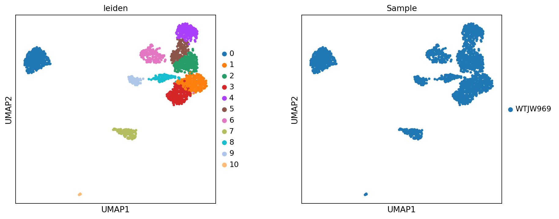

output

11 components passed P cutoff of 0.1.

Per-cell sequencing depth and methylation levels

Figure legend: QC metrics shown on the methylation UMAP.

• reads_counts: per-cell sequencing depth (number of mapped reads).
• CpG%: per-cell CpG methylation ratio.
• CH%: per-cell CH methylation ratio.

Tip: Use the colorbar to interpret how colors map to numeric values.

sc.set_figure_params(scanpy=True, fontsize=12, facecolor='white', figsize=(5, 5), dpi=80)
sc.pl.umap(adata_met, color = ['reads_counts','CpG%','CH%'])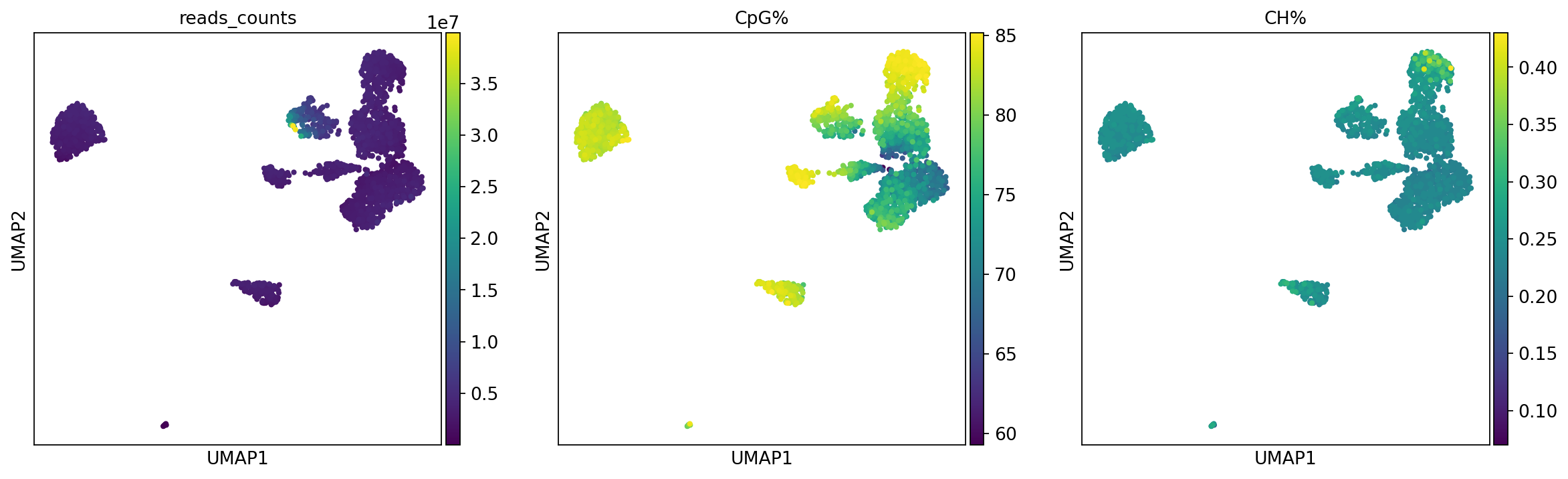

Correlation between LSI components and QC metrics

In single-cell methylation, the first LSI component often correlates with sequencing depth and other technical factors. Before downstream steps, it is useful to check correlations between LSI components and QC metrics such as reads_counts and CpG%.

If a component is strongly driven by technical variation, consider excluding it when building the neighbor graph (a common practice is to drop the first LSI component).

# Calculate the correlation between LSI components and sequencing depth (reads_counts) and methylation level (CpG%)
lsi_mat = adata_met.obsm[met_reduc_use]
n_components = lsi_mat.shape[1]
components = [f"{met_reduc_use}_{i}" for i in range(n_components)]

# Prepare data
metrics = ['reads_counts', 'CpG%']
cor_data = []

for metric in metrics:
    if metric in adata_met.obs.columns:
        # Calculate correlation coefficient between each LSI column and metric
        corrs = [np.corrcoef(lsi_mat[:, i], adata_met.obs[metric])[0, 1] for i in range(n_components)]
        cor_data.append(corrs)

cor_df = pd.DataFrame(cor_data, index=[m for m in metrics if m in adata_met.obs.columns], columns=components)

# Plotting
fig, ax = plt.subplots(figsize=(11, 3), dpi = 80)
im = ax.imshow(cor_df, cmap='coolwarm', vmin=-1, vmax=1)
ax.set_yticks(np.arange(len(cor_df.index)))
ax.set_yticklabels(cor_df.index)
ax.set_xlabel("LSI Components")
ax.set_title("Correlation between LSI Components and QC Metrics")
plt.colorbar(im, label="Pearson Correlation")
plt.grid(False)
plt.tight_layout()
plt.show()

# Print components highly correlated with reads_counts
if 'reads_counts' in cor_df.index:
    print("Top LSI components correlated with reads_counts:")
    print(cor_df.loc['reads_counts'].abs().sort_values(ascending=False).head())

# Print components highly correlated with reads_counts
if 'CpG%' in cor_df.index:
    print("Top LSI components correlated with CpG%:")
    print(cor_df.loc['CpG%'].abs().sort_values(ascending=False).head())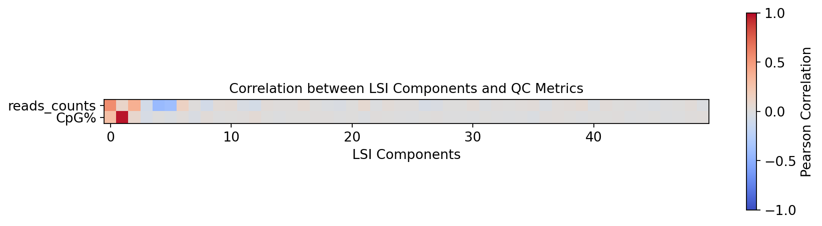

Top LSI components correlated with reads_counts:
X_lsi_0    0.559620
X_lsi_4    0.423008
X_lsi_5    0.397521
X_lsi_2    0.377632
X_lsi_6    0.137376
Name: reads_counts, dtype: float64
Top LSI components correlated with CpG%:
X_lsi_1     0.967854
X_lsi_0     0.284859
X_lsi_2     0.085100
X_lsi_3     0.049610
X_lsi_12    0.041342
Name: CpG%, dtype: float64

RNA Data Preprocessing

Transcriptome preprocessing workflow

RNA preprocessing follows a commonly used Scanpy workflow. The goal is to remove low-quality cells/genes, reduce technical variation, and keep major biological variation:

1. Quality control (QC):
   • sc.pp.filter_cells: filter cells with too few detected genes.
   • sc.pp.filter_genes: filter genes detected in very few cells.
   • Mitochondrial/ribosomal/hemoglobin ratios: compute these as helpful QC indicators; a high mitochondrial fraction often suggests stressed or damaged cells.
2. Normalization:
   • sc.pp.normalize_total: normalize total counts per cell (commonly to 10,000) to reduce depth-related effects.
3. Log transform:
   • sc.pp.log1p: apply $\log (x+1)$ to compress dynamic range and stabilize variance.
4. Highly variable genes (HVGs):
   • sc.pp.highly_variable_genes: select informative genes with high cell-to-cell variation to reduce noise and computation.
5. Scaling:
   • sc.pp.scale: scale each gene to mean 0 and variance 1 to prevent highly expressed genes from dominating PCA.
6. PCA (sc.tl.pca): compute principal components in HVG space.
7. Batch correction (optional): if multiple samples are included, use Harmony (run_harmony) in PCA space to mitigate batch effects.

adata_rna

output

AnnData object with n_obs × n_vars = 2189 × 38606
obs: 'orig.ident', 'nCount_RNA', 'nFeature_RNA', 'mito', 'Sample', 'raw_Sample', 'resolution.0.5_d30', 'CellAnnotation', 'original_barcode', 'chemistry'
var: 'gene_ids', 'feature_types'

# 1. Filter low-quality cells and genes
# min_genes=200: Filter out cells with fewer than 200 detected genes (possibly dead cells or empty droplets)
sc.pp.filter_cells(adata_rna, min_genes=200)
# min_cells=3: Filter out genes expressed in fewer than 3 cells (possibly sequencing noise)
sc.pp.filter_genes(adata_rna, min_cells=3)

# 2. Calculate QC metrics
# Mitochondrial genes: Usually start with 'MT-' (Human)
adata_rna.var["mt"] = adata_rna.var_names.str.startswith("MT-")
# Ribosomal genes: Usually start with 'RPS' or 'RPL'
adata_rna.var["ribo"] = adata_rna.var_names.str.startswith(("RPS", "RPL"))
# Hemoglobin genes: Usually start with 'HB'
adata_rna.var["hb"] = adata_rna.var_names.str.contains("^HB[^(P)]")

# Calculate QC metrics, results will be stored in adata_rna.obs and adata_rna.var
sc.pp.calculate_qc_metrics(adata_rna, qc_vars=["mt", "ribo", "hb"], inplace=True, log1p=True)

# Backup raw counts data for differential gene analysis, etc.
adata_rna.layers["counts"] = adata_rna.X.copy()

# 1. Normalization
# Standardize the sequencing depth of each cell (usually scaled to 10,000 reads)
sc.pp.normalize_total(adata_rna, target_sum=1e4)

# 2. Log Transformation
# log(x+1) transformation to stabilize variance and make data approximately normal
sc.pp.log1p(adata_rna)

# 3. Highly Variable Gene Selection (Feature Selection)
# Select genes with significant expression differences across cells (HVGs), picking the top 2000 here
sc.pp.highly_variable_genes(adata_rna, flavor='seurat_v3', n_top_genes=2000, batch_key="Sample")

# 4. Data Scaling
# Scale the expression of each gene to a mean of 0 and variance of 1, ensuring highly expressed genes do not dominate PCA
sc.pp.scale(adata_rna, max_value=10)

# 5. PCA Dimensionality Reduction
# Perform principal component analysis in HVG space to extract main variation axes
sc.tl.pca(adata_rna, svd_solver='arpack')

# 6. Batch Correction (Harmony Integration)
# Perform batch correction only when multiple samples exist
if len(samples) > 1:
    print("Running Harmony for batch correction...")
    ho = run_harmony(
        adata_rna.obsm['X_pca'],
        meta_data=adata_rna.obs,
        vars_use='Sample',
        random_state=0,
        max_iter_harmony=20
    )
    # Store the corrected PCA coordinates in obsm
    adata_rna.obsm['X_pca_harmony'] = ho.Z_corr
    rna_reduc_use = 'X_pca_harmony'
else:
    print("Only one sample detected, skipping batch correction.")
    rna_reduc_use = 'X_pca'

# 7. Compute Neighbors Graph
# Compute neighbor relationships between cells based on the selected dimensionality reduction result (X_pca or X_pca_harmony)
sc.pp.neighbors(adata_rna, use_rep=rna_reduc_use, n_neighbors=15, n_pcs=30, random_state=20)

# 8. UMAP Dimensionality Reduction and Clustering
# UMAP is used for visualization, Leiden for clustering
sc.tl.umap(adata_rna, random_state=20)
# sc.tl.tsne(adata_rna, use_rep=rna_reduc_use, random_state=20) # Optional t-SNE
sc.tl.leiden(adata_rna, resolution=resolution, random_state=20)

output

Only one sample detected, skipping batch correction.

Clustering results based on transcriptome (RNA)

• If samples are clearly separated on UMAP, it often indicates batch effects; Harmony can help.
• If samples are already well mixed, Harmony may have little impact.

Note: Harmony mainly corrects sample/batch differences. If upstream QC, filtering, or normalization is insufficient, or some samples have much lower quality, batch correction will be limited.

Figure legend: RNA UMAP (clusters and samples). This plot shows the RNA modality in UMAP space, colored by leiden (clusters) and Sample (samples).

• Axes: UMAP1 and UMAP2.
• Color (leiden): cluster labels.
• Color (Sample): sample labels, useful for checking batch effects.
• Dots: each dot is a cell.

sc.set_figure_params(scanpy=True, fontsize=12, facecolor='white', figsize=(5, 5), dpi=80)
sc.pl.umap(adata_rna, color = ['leiden','Sample'], wspace=0.3)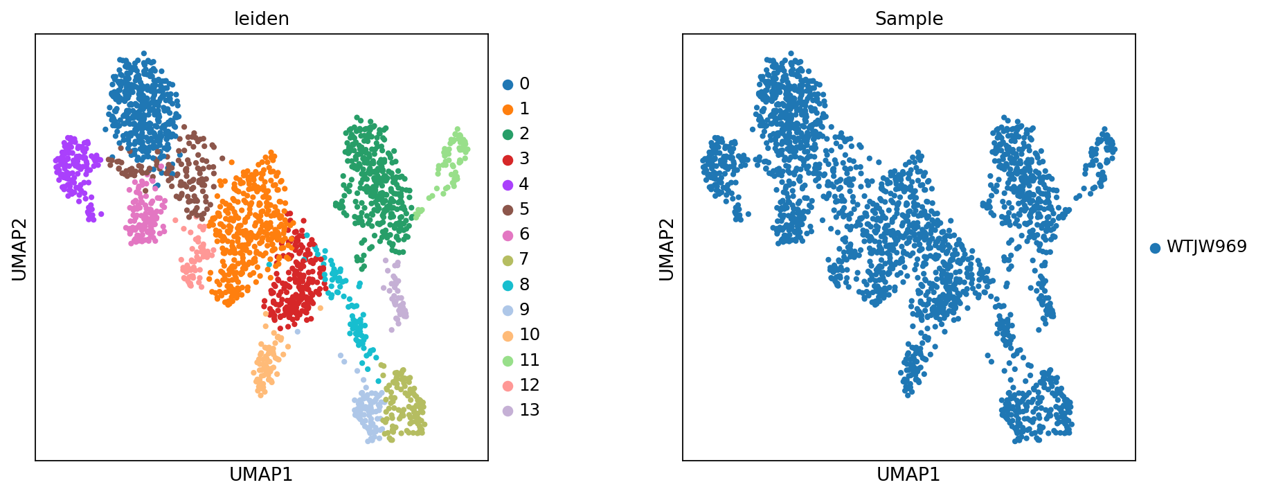

Figure legend: RNA UMAP (marker gene expression). This plot shows the expression of marker genes on the RNA UMAP.

• Axes: UMAP1 and UMAP2.
• Color: gene expression level; use the colorbar for interpretation.
• Dots: each dot is a cell.

Tip: Example markers include CD3D, THEMIS (T cells), NKG7 (NK cells), CD8A (CD8+ T cells), CD4 (CD4+ T cells), CD79A and MS4A1 (B cells), JCHAIN (plasma cells), LYZ (monocytes), and LILRA4 (pDC cells).

colors = ["#F5E6CC", "#FDBB84", "#E34A33", "#7F0000"]
my_warm_cmap = mcolors.LinearSegmentedColormap.from_list("white_orange_red", colors, N=256)

marker_names = ["CD3D", "THEMIS", "NKG7", "CD8A", "CD4", "IL7R", "S100A4", "CCR7",
                "CD79A","MS4A1","JCHAIN",
                "LYZ","FCN1","FCGR3A","CST3","MKI67"]
sc.pl.umap(
    adata_rna, 
    color=marker_names, 
    ncols=4,            
    color_map=my_warm_cmap, 
    vmax='p99',         
    s=10,               
    frameon=False,      
    vmin=0,
    show=False 
)

plt.gcf().set_size_inches(12, 8) 
plt.show()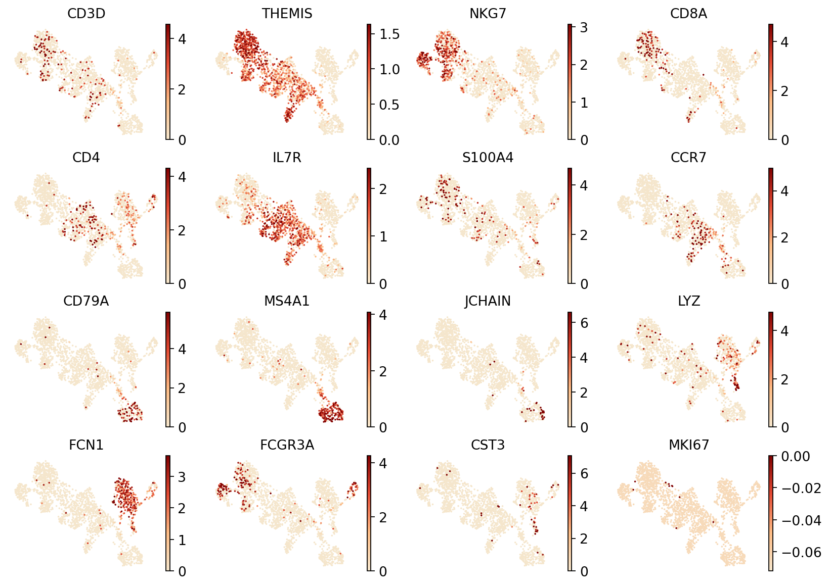

celltype = {
    '0': 'CD8+ T',
    '1': 'Navie CD4+ T',
    '2': 'CD14+ Mono',
    '3': 'Memory CD4+ T',
    '4': 'NK',
    '5': 'T',
    '6': 'T',
    '7': 'B',
    '8': 'Multiplet',
    '9': 'B',
    '10': 'Memory CD4+ T',
    '11': 'FCGR3A+ Mono',
    '12': 'Navie CD4+ T',
    '13': 'DC'
}

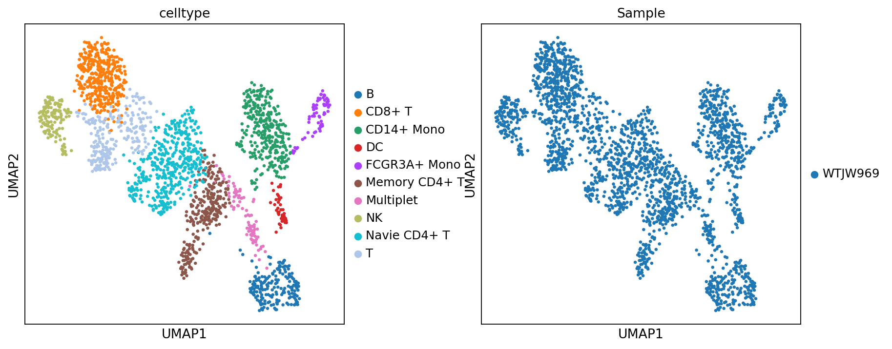
adata_rna.obs['celltype'] = adata_rna.obs['leiden'].map(celltype)

Figure legend: RNA UMAP (cell types and samples). This plot shows the RNA modality in UMAP space, colored by celltype (cell types) and Sample (samples).

• Axes: UMAP1 and UMAP2.
• Color (celltype): annotated cell types.
• Color (Sample): sample labels, useful for checking batch effects and sample composition.
• Dots: each dot is a cell.

sc.set_figure_params(scanpy=True, fontsize=12, facecolor='white', figsize=(5, 5), dpi = 80)
sc.pl.umap(
    adata_rna, 
    color=['celltype', 'Sample'], 
    ncols=2,
    s=35,
    wspace=0.3
)

WNN Multi-omics Integration Analysis

WNN principles and steps

In this section, we put RNA and methylation into a single MuData container, then use WNN (Weighted Nearest Neighbors) to build a joint neighbor graph for downstream embedding and clustering.

Core steps:

1. Build a multi-omics container: use mu.MuData to encapsulate RNA (mdata['rna']) and methylation (mdata['methy']).
2. Compute single-modality neighbors:
   • RNA: compute neighbors using a PCA representation (X_pca or X_pca_harmony).
   • Methylation: compute neighbors using an LSI representation (X_lsi or X_lsi_harmony).
3. WNN fusion (mu.pp.neighbors):
   • For each cell, the algorithm compares local neighborhood structure across modalities and learns cell-specific modality weights.
   • It then fuses neighbor information using these weights and writes a set of results under key_added='wnn' (typically mdata.uns['wnn'], plus adjacency matrices stored in mdata.obsp).
4. Joint embedding and clustering:
   • UMAP (mu.tl.umap): compute a unified 2D embedding from the WNN graph.
   • Leiden (mu.tl.leiden or sc.tl.leiden): identify clusters on the WNN graph.

A practical benefit of WNN is that it can adaptively use complementary signals: some cells may be better separated by RNA, while others may carry stronger structure in methylation.

# Build multi-omics MuData object
mdata = mu.MuData({
    'rna': adata_rna, 
    'methy': adata_met})

Choose the number of informative components

Before building the WNN graph, we need to decide how many components to use for each modality:

• RNA: number of PCA components.
• Methylation: number of LSI components.

Here we use significant_pc_test to estimate how many components are likely to contain meaningful biological signal.

• p_cutoff=0.1: significance threshold.

rna_sig_pcs = significant_pc_test(adata_rna, obsm=rna_reduc_use, update=False, p_cutoff=0.1)
met_sig_pcs = significant_pc_test(adata_met, obsm=met_reduc_use, update=False, p_cutoff=0.1)

print(f"Significant PCs for RNA: {rna_sig_pcs}")
print(f"Significant LSI components for Methylation: {met_sig_pcs}")

output

12 components passed P cutoff of 0.1.
11 components passed P cutoff of 0.1.
Significant PCs for RNA: 12
Significant LSI components for Methylation: 11

Run WNN

This step computes neighbors in each modality and then fuses them into a WNN graph.

• Use the selected number of components (n_pcs) to compute neighbors for RNA (PCA) and methylation (LSI).
• Run mu.pp.neighbors to build the WNN graph, then run UMAP and Leiden clustering on that graph.

sc.pp.neighbors(mdata['rna'], use_rep=rna_reduc_use, n_pcs=rna_sig_pcs)
sc.pp.neighbors(mdata['methy'], use_rep=met_reduc_use, n_pcs=met_sig_pcs)

# 2. Build the WNN graph and estimate modality weights
# Results are written under key_added='wnn' (commonly mdata.uns['wnn'], plus adjacency matrices in mdata.obsp)
# Modality weights are also added per cell (column names are typically prefixed by modality, e.g., rna:mod_weight, methy:mod_weight)
mu.pp.neighbors(mdata, key_added='wnn', add_weights_to_modalities=True, random_state=20)

# 3. Keep the intersection of cells across modalities (ensure both modalities use the same cells)
mu.pp.intersect_obs(mdata)

# 4. Run UMAP and clustering (Leiden) on the WNN graph
mu.tl.umap(mdata, neighbors_key='wnn', random_state=20)
sc.tl.leiden(mdata, neighbors_key='wnn', random_state=20)

mdata.obsm["X_wnn_umap"] = mdata.obsm["X_umap"]

sc.set_figure_params(scanpy=True, fontsize=12, facecolor='white', figsize=(5, 5), dpi = 80)
mu.pl.embedding(mdata, basis="X_wnn_umap", color=["rna:mod_weight", "methy:mod_weight"], wspace=0.3)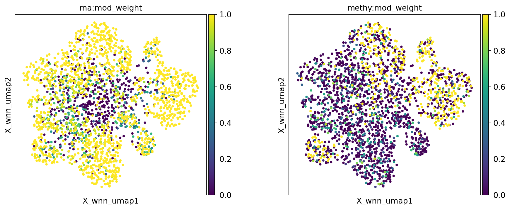

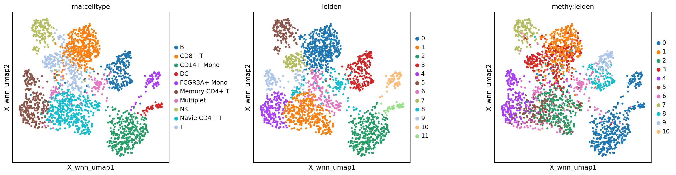
WNN embedding and clustering results

Figure legend: Comparison across modalities.

• Left panel: RNA-only cell type annotation (rna:celltype).
• Middle panel: WNN clustering (wnn:leiden).
• Right panel: methylation-only clustering (methy:leiden).

sc.set_figure_params(scanpy=True, fontsize=12, facecolor='white', figsize=(5, 5), dpi = 80)
mu.pl.embedding(mdata, basis="X_wnn_umap", color=["rna:celltype", "leiden", "methy:leiden"], wspace=0.4)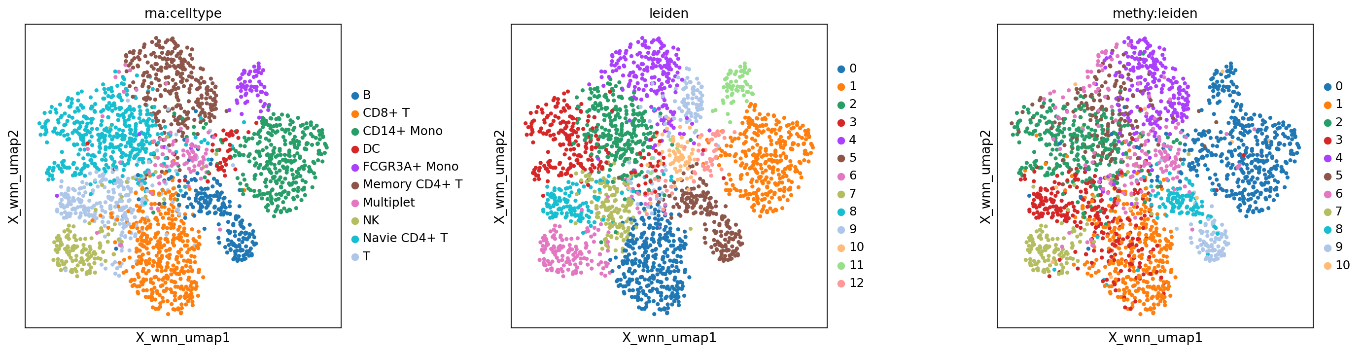

Parameter tuning (optional)

If the initial clustering is not satisfactory (for example, distinct cell populations remain mixed, or expected subpopulations are not separated), the number of components used to build the graph may be too small.

You can try increasing n_pcs (PCA components for RNA or LSI components for methylation), then rebuild the WNN graph and re-run UMAP and clustering.

Tip: Do not increase the number too aggressively; too many components can add noise and lead to over-clustering.

# Manually specify more PCs/LSI components to improve resolution
# Note: The number of n_pcs should not exceed the total number of principal components/LSI components (usually 50 or 30)
print("Re-running WNN with manually adjusted n_pcs...")
sc.pp.neighbors(mdata['rna'], use_rep=rna_reduc_use, n_pcs=20)  # RNA increased to 20
sc.pp.neighbors(mdata['methy'], use_rep=met_reduc_use, n_pcs=50) # Methylation increased to 50 (maximum)

# Re-compute WNN graph
mu.pp.neighbors(mdata, key_added='wnn', add_weights_to_modalities=True, random_state=20)
mu.pp.intersect_obs(mdata)

# Re-run UMAP and clustering
mu.tl.umap(mdata, neighbors_key='wnn', random_state=20)
sc.tl.leiden(mdata, neighbors_key='wnn', random_state=20)

# Save new UMAP coordinates
mdata.obsm["X_wnn_umap"] = mdata.obsm["X_umap"]

# Visualize new results
sc.set_figure_params(scanpy=True, fontsize=12, facecolor='white', figsize=(5, 5), dpi=80)
mu.pl.embedding(mdata, basis="X_wnn_umap", color=["rna:mod_weight", "methy:mod_weight"], wspace=0.3)

sc.set_figure_params(scanpy=True, fontsize=12, facecolor='white', figsize=(5, 5), dpi=80)
mu.pl.embedding(mdata, basis="X_wnn_umap", color=["rna:celltype", "leiden", "methy:leiden"], wspace=0.4)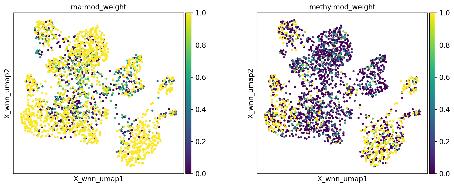

output

Re-running WNN with manually adjusted n_pcs...

Saving outputs

After the analysis, save processed data objects in standard formats for reuse and downstream analysis.

Files saved:

• adata_rna.h5ad: RNA modality object with preprocessing, embedding, clustering, and annotations.
• adata_met.h5ad: methylation modality object with preprocessing, embedding, and clustering.
• mdata.h5mu: MuData object containing both modalities and WNN results.

Note:

• .h5ad and .h5mu preserve the full analysis state and can be loaded later for visualization or downstream analysis.
• These files can be large; make sure the output directory has enough disk space.

adata_rna.write_h5ad(f'{outdir}/adata_rna.h5ad')
adata_met.write_h5ad(f'{outdir}/adata_met.h5ad')
mdata.write(f'{outdir}/mdata.h5mu')