scRNA-seq + scATAC-seq Multimodal Data Integration Tutorial

Author: SeekGene

Time: 15 min

Words: 2.9k words

Updated: 2025-11-20

Reads: 0 times

This tutorial is designed for beginners and demonstrates how to integrate two types of single-cell data using Seurat and Signac:

• scRNA-seq: measures gene expression (which genes are "on" in each cell)
• scATAC-seq: measures chromatin accessibility (which DNA regions are "open" in each cell)

The core goal of integration is to "transfer" (label transfer) annotated scRNA-seq cell labels to scATAC-seq, thus automatically annotating ATAC cells. Subsequently, a "co-embedding" step can embed both cell types into the same reduced dimensional space for joint visualization (mainly for visualization purposes).

Before using this tutorial, it is recommended to prepare:

• Annotated scRNA-seq data (for example, with cell_type or cluster labels)
• The same species and compatible genome build and chromosome naming conventions as your scATAC-seq data (e.g., hg38, chr1 format)
• A basic R running environment and sufficient memory

In this tutorial, we will learn how to:

1. Data Loading: Read scRNA-seq and scATAC-seq data separately
2. Data Preprocessing: Perform quality control (QC) and initial filtering
3. Data Normalization: Prepare for integration (normalization and selection of variable genes for RNA; TF-IDF/LSI for ATAC)
4. Gene Activity Score: Convert ATAC peaks to a gene activity matrix approximating "expression"
5. Cross-Modal Integration: Perform label transfer by anchor matching
6. Visualization and Export: UMAP/co-embedding for visualization and result saving

# Load required R packages
suppressPackageStartupMessages({
  library(Seurat)
  library(Signac)
  library(EnsDb.Hsapiens.v86)
  library(BSgenome.Hsapiens.UCSC.hg38)
  library(biovizBase)
  #library(BSgenome.Mmusculus.UCSC.mm10)
  #library(EnsDb.Mmusculus.v79)
  library(dplyr)
  library(ggplot2)
  library(patchwork)
})

# Set random seed
set.seed(1234)

# Set Seurat options (note: 8000 * 1024^2 is actually 8GB)
options(future.globals.maxSize = 8000 * 1024^2)  # 8GB

my36colors <-c( '#E5D2DD', '#53A85F', '#F1BB72', '#F3B1A0', '#D6E7A3', '#57C3F3', '#476D87',
                '#E95C59', '#E59CC4', '#AB3282', '#23452F', '#BD956A', '#8C549C', '#585658',
                '#9FA3A8', '#E0D4CA', '#5F3D69', '#C5DEBA', '#58A4C3', '#E4C755', '#F7F398',
                '#AA9A59', '#E63863', '#E39A35', '#C1E6F3', '#6778AE', '#91D0BE', '#B53E2B',
                '#712820', '#DCC1DD', '#CCE0F5', '#CCC9E6', '#625D9E', '#68A180', '#3A6963',
                '#968175', "#6495ED", "#FFC1C1",'#f1ac9d','#f06966','#dee2d1','#6abe83','#39BAE8','#B9EDF8','#221a12',
                '#b8d00a','#74828F','#96C0CE','#E95D22','#017890')

1. Data Loading and Preparation

For ease of use, this tutorial follows the standard 10x Genomics directory structure. Please prepare the following files:

scRNA-seq data (expression matrix)
├── RNA_sample
│ ├── filtered_feature_bc_matrix
│ │ ├── barcodes.tsv.gz (cell barcodes)
│ │ ├── features.tsv.gz (gene list)
│ │ └── matrix.mtx.gz (sparse expression matrix)

scATAC-seq data (peaks matrix + fragments)
├── ATAC_sample
│ ├── filtered_peaks_bc_matrix
│ │ ├── barcodes.tsv.gz (cell barcodes)
│ │ ├── features.tsv.gz (peaks list)
│ │ └── matrix.mtx.gz (sparse count matrix)
│ ├── ATAC_sample_fragments.tsv.gz (genomic coordinates of each sequencing fragment, for TSS enrichment/nucleosome signal QC)
│ ├── ATAC_sample_fragments.tsv.gz.tbi (index file for fragments)
│ └── per_barcode_metrics.csv (optional QC metrics per cell)

Tips:

• If you use data generated from a different platform or pipeline, make sure they can be loaded equivalently as a sparse matrix and fragment file.
• Try to ensure that the RNA and ATAC samples come from similar conditions/samples for more reliable label transfer.

Obtain Gene Annotation Information

We will retrieve human genome annotation (gene location, transcripts, exons, TSS, etc.) from the EnsDb database. This information is used for:

• Calculating ATAC TSS enrichment (to assess whether open chromatin is concentrated near transcription start sites)
• Constructing the "gene activity matrix" (mapping peak signals to genes) Please make sure:
• The species and reference genome version match (e.g., EnsDb.Hsapiens.v86 corresponds to hg38)
• Chromosome naming conventions are consistent (for example, all use prefixes like chr1, chr2)

# Obtain gene annotation information (suppress warnings and messages)
suppressWarnings({
  suppressMessages({
    annotation <- GetGRangesFromEnsDb(ensdb = EnsDb.Hsapiens.v86)
    seqlevels(annotation) <- paste0('chr', seqlevels(annotation))
    genome(annotation) <- 'hg38'
  })
})

# Set up parallel computing (silent, optional)
suppressPackageStartupMessages({
  library(future)
})
plan("multicore", workers = 4)

Read scRNA-seq Data

We will read in the 10x expression matrix (barcodes/features/matrix), and create a standard Seurat object:

• counts: gene counts for each cell
• meta.data: sample information, QC metrics, clustering/cell type data, etc. will be added later

The resulting object will serve as the "reference" for transferring labels to the ATAC cells.

options(warn = -1)
# Define scRNA-seq data path
rna_sample_name <- 'joint34'
rna_counts_path <- file.path(rna_sample_name, 'filtered_feature_bc_matrix')

# Read scRNA-seq data
rna_counts <- Read10X(rna_counts_path)

# Create scRNA-seq Seurat object
rna_obj <- CreateSeuratObject(
  counts = rna_counts,
  project = "RNA_sample",
  min.cells = 3,
  min.features = 200
)

# Add sample identifiers
rna_obj$orig.ident <- 'joint34'
rna_obj$Sample <- 'joint34'
rna_obj$technology <- 'RNA'
options(warn = 0)
# scRNA-seq data reading completed

Read scATAC-seq Data

Here we will read in:

• filtered_peaks_bc_matrix: a sparse matrix of peaks × cells (represents counts of open chromatin)
• fragments.tsv.gz: genomic coordinates of each sequenced fragment (used for TSS enrichment, nucleosome signal, and other QC)

We then use Signac to create a ChromatinAssay, which is wrapped into a Seurat object. This object will serve as the "query" to receive transferred RNA labels.

# Define scATAC-seq data path
atac_sample_name <- 'joint41'
atac_counts_path <- file.path(atac_sample_name, 'filtered_peaks_bc_matrix')
atac_fragments_path <- file.path(atac_sample_name, paste0(atac_sample_name, '_A_fragments.tsv.gz'))
#atac_metadata_path <- file.path(atac_sample_name, 'per_barcode_metrics.csv')

# Read scATAC-seq data
atac_counts <- Read10X(atac_counts_path)

# Read quality control metadata
#atac_metadata <- read.csv(
#  file = atac_metadata_path,
#  header = TRUE,
#  row.names = 1
#)

# Create ChromatinAssay object
chrom_assay <- CreateChromatinAssay(
  counts = atac_counts,
  sep = c(':', '-'),
  fragments = atac_fragments_path,
  annotation = annotation,
  min.cells = 3,
  min.features = 200
)

# Create scATAC-seq Seurat object
atac_obj <- CreateSeuratObject(
  counts = chrom_assay,
  assay = "ATAC",
  project = "ATAC_sample"#,meta.data = atac_metadata
)

# Add sample identifiers
atac_obj$orig.ident <- 'joint41'
atac_obj$Sample <- 'joint41'
atac_obj$technology <- 'joint41'

# scATAC-seq data reading completed

2. Data Preprocessing

Before integration, we need to "clean" both types of data separately:

• QC (Quality Control): Remove low-quality cells (e.g., high mitochondrial gene percentage, low TSS enrichment for ATAC, etc.)
• Initial Normalization/Dimensionality Reduction: Prepare for anchor finding and visualization in later steps

Thresholds will vary across datasets. Below we introduce common QC metrics and visualization methods to help you empirically adjust thresholds based on their distributions.

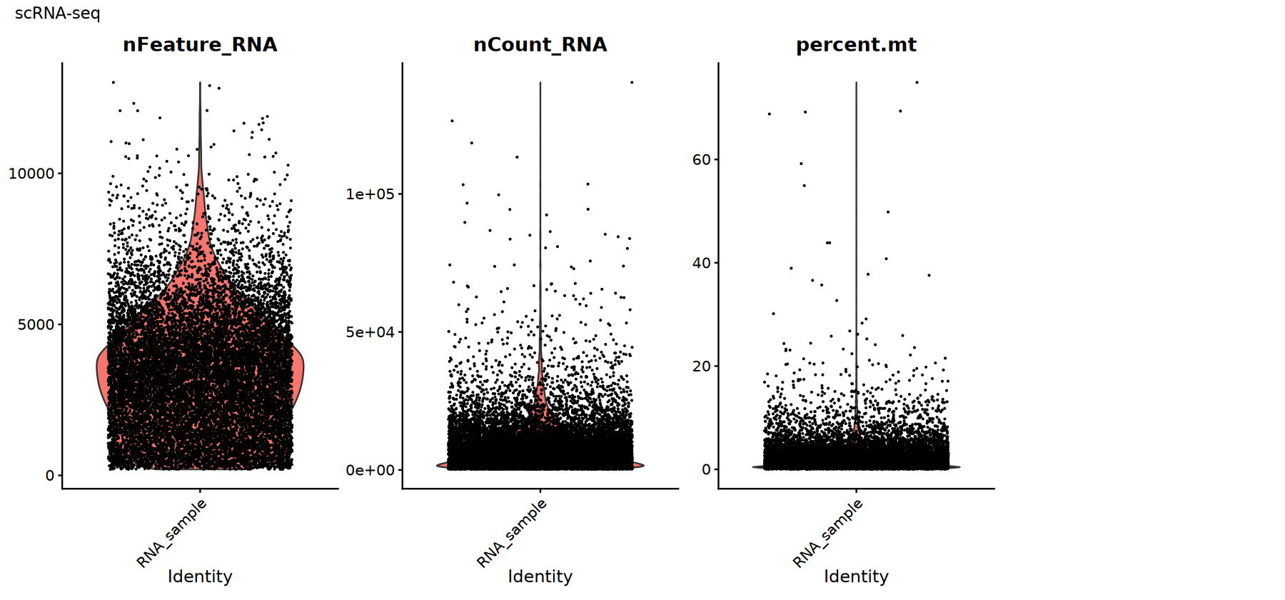
scRNA-seq Data Quality Control

Common QC metrics:

• percent.mt: percentage of mitochondrial genes. A high value usually indicates damaged cells or RNA leakage.
• nFeature_RNA: number of detected genes. A low value may suggest empty droplets, while a high value could indicate doublets/multiplets.
• nCount_RNA: total counts. This relates to sequencing depth and should be assessed based on its distribution to flag outliers.

There are no universal cutoffs for these metrics. Thresholds should be empirically determined based on their distributions (e.g., using violin/scatter plots).

# Calculate the proportion of mitochondrial gene expression
suppressWarnings({
    rna_obj[["percent.mt"]] <- PercentageFeatureSet(rna_obj, pattern = "^MT-")
})

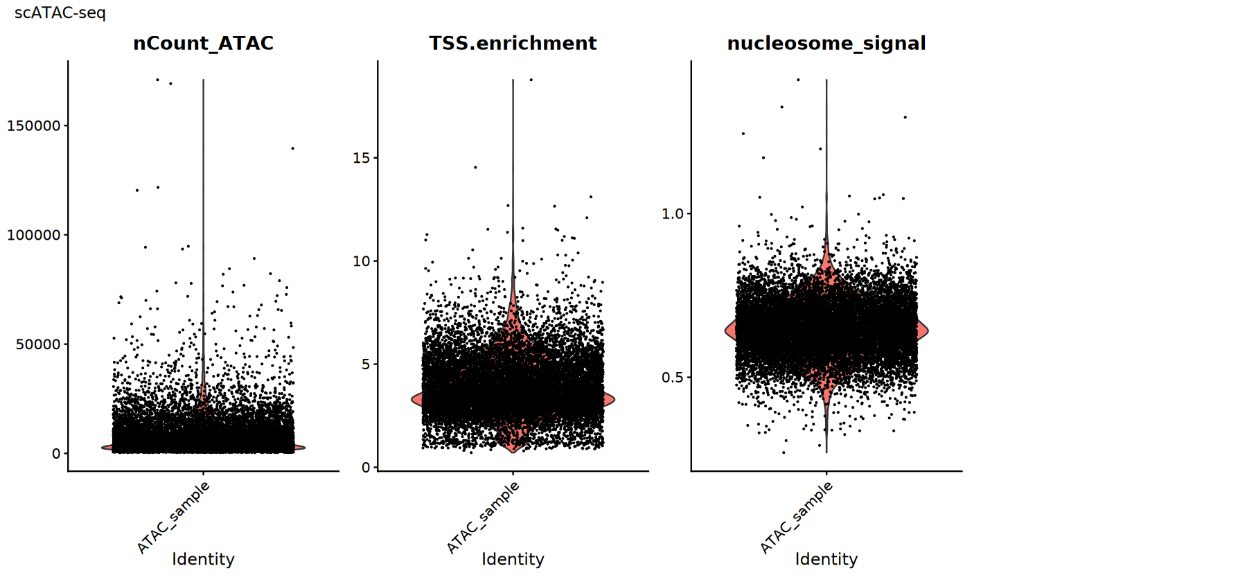
scATAC-seq Data Quality Control

Common QC metrics:

• TSS.enrichment: (Transcription Start Site enrichment score) Higher values are better, indicating a stronger signal concentrated near transcription start sites; low values may suggest high background or low cell activity.
• nucleosome_signal: Reflects the periodic signal of nucleosomes; typically, lower values are better.
• nCount_ATAC: Total ATAC counts; both extremely low or high values can indicate abnormal cells.

Thresholds should be set based on the data distribution and supplemented with fragment quality, doublet rates, and other factors.

# Set the default assay to "ATAC"
DefaultAssay(atac_obj) <- 'ATAC'

# Calculate TSS enrichment score
atac_obj <- TSSEnrichment(atac_obj)

# Calculate nucleosome signal
atac_obj <- NucleosomeSignal(atac_obj)

QC Visualization

Use violin plots to examine the distribution/outliers of QC metrics and aid in threshold selection:

• RNA: nFeature_RNA, nCount_RNA, percent.mt
• ATAC: nCount_ATAC, TSS.enrichment, nucleosome_signal

Recommendations:

• Look for obvious long tails or bimodal distributions
• Try several sets of thresholds and compare whether downstream clustering/UMAP is clearer

# Visualization of scRNA-seq QC metrics
suppressWarnings({
    options(repr.plot.width = 15, repr.plot.height = 7)
    p1 <- VlnPlot(rna_obj, 
              features = c("nFeature_RNA", "nCount_RNA", "percent.mt"),
              ncol = 4, pt.size = 0.1) +
      plot_annotation(title = "scRNA-seq")

    print(p1)

    # Visualization of scATAC-seq QC metrics
    p2 <- VlnPlot(atac_obj, 
              features = c("nCount_ATAC", "TSS.enrichment", "nucleosome_signal"),
              ncol = 4, pt.size = 0.1) +
      plot_annotation(title = "scATAC-seq")

    print(p2)
})

Quality Control Filtering

Choose thresholds based on the previous distribution plots and filter out low-quality cells. Tips:

• A decrease in cell number after filtering is normal; the key is to improve the signal-to-noise ratio.
• Record the thresholds used and your rationale for reproducibility and team communication.

# scRNA-seq data filtering
cat('Number of scRNA-seq cells before filtering:', ncol(rna_obj), '\n')
rna_obj <- subset(rna_obj, 
                  subset = nFeature_RNA > 200 & 
                          nFeature_RNA < 10000 & 
                          percent.mt < 20)
cat('Number of scRNA-seq cells after filtering:', ncol(rna_obj), '\n')
# scATAC-seq data filtering
cat('Number of scATAC-seq cells before filtering:', ncol(atac_obj), '\n')
atac_obj <- subset(atac_obj,
                   subset = nCount_ATAC > 500 &
                           nCount_ATAC < 50000 &
                           TSS.enrichment > 1 &
                           nucleosome_signal < 1)
cat('Number of scATAC-seq cells after filtering:', ncol(atac_obj), '\n')

Data Normalization and Dimensionality Reduction

We will preprocess and normalize each data type separately using appropriate methods:

• RNA: Normalize → Select variable genes → Scale → PCA/UMAP → Neighbor graph and clustering
• ATAC: TF-IDF → Select important features (peaks) → LSI (a PCA-like method) → UMAP

Purpose: Bring samples with different sequencing depths and count ranges into a comparable space, preliminarily reveal principal structure, and facilitate subsequent identification of "cross-modal anchors".

# scRNA-seq数据标准化处理
suppressWarnings({
  suppressMessages({
      rna_obj <- NormalizeData(rna_obj)
      rna_obj <- FindVariableFeatures(rna_obj,nfeatures=4000)
      rna_obj <- ScaleData(rna_obj)
      rna_obj <- RunPCA(rna_obj)
      rna_obj <- RunUMAP(rna_obj, dims = 1:30)
      rna_obj <- FindNeighbors(rna_obj, dims = 1:30)
      rna_obj <- FindClusters(rna_obj, resolution = 0.5)
  })
})

# scATAC-seq data normalization and processing
suppressWarnings({
  suppressMessages({
      atac_obj <- RunTFIDF(atac_obj)
      atac_obj <- FindTopFeatures(atac_obj, min.cutoff = "q0")
      atac_obj <- RunSVD(atac_obj)
      atac_obj <- RunUMAP(atac_obj, reduction = "lsi", dims = 2:30, reduction.name = "umap.atac", reduction.key = "atacUMAP_")
  })
})

3. Gene Activity Score Calculation

To connect the "chromatin accessibility" from ATAC with the "gene expression level" from RNA, we need to map peak signals to genes and obtain "gene activity scores". While this is not a direct measurement of expression, it can statistically approximate a gene's potential activity, serving as a crucial bridge for cross-modality integration.

Calculate Gene Activity Matrix

Idea: Aggregate the peak signals associated with each gene (covering gene body plus promoter regions upstream and downstream of the TSS) to get a "gene activity score" for each gene in each cell.

• A typical approach uses a window of ~2kb upstream and ~1kb downstream of the TSS (this can be adjusted as needed)
• The resulting ACTIVITY assay will be used to establish anchors with the RNA RNA assay

# Calculate gene activity scores
# Use gene body and promoter regions to calculate activity scores
suppressWarnings({
    DefaultAssay(atac_obj)="ATAC"
    gene.activities <- GeneActivity(
        object = atac_obj,
        features = VariableFeatures(rna_obj),extend.upstream = 2000,extend.downstream = 1000)

    # Add the gene activity matrix as a new assay
    atac_obj[['ACTIVITY']] <-  CreateAssayObject(counts = gene.activities)
    DefaultAssay(atac_obj) <- "ACTIVITY"
    # Normalize gene activity data
    atac_obj <- NormalizeData(atac_obj)
    atac_obj <- ScaleData(atac_obj, features = rownames(atac_obj))
})

4. Multimodal Data Integration

Now we perform cross-modality matching between the "RNA expression matrix (reference)" and the "ATAC gene activity matrix (query)". The core tasks are:

• Identify cross-modality correspondences ("anchors")
• Transfer cell labels from the reference to the query cells

Find Integration Anchors

"Anchors" are key to aligning two data spaces. The approach is to use methods such as CCA or LSI to identify highly comparable subspaces between the RNA and ATAC (gene activity) matrices, thereby establishing coordinate systems that can be projected onto each other.

# Set the default assay of the scATAC-seq object to ACTIVITY (gene activity scores)
DefaultAssay(atac_obj) <- 'ACTIVITY'
suppressWarnings({
  suppressMessages({
      # Find integration anchors
      transfer.anchors <- FindTransferAnchors(
          reference = rna_obj,
          query = atac_obj,
          features = VariableFeatures(object = rna_obj),
          reference.assay = 'RNA',
          query.assay = 'ACTIVITY',
          k.anchor = 30,
          k.filter = 50 ,
          reduction = 'cca'
      )
  })
})

Predict cell type labels

Once the anchors are established, you can transfer the "reference" labels (e.g., cell_type or seurat_clusters) to the ATAC cells:

• The output predicted.id gives the predicted cell type/cluster for each ATAC cell
• You can also obtain prediction scores, which provide a measure of confidence (this tutorial shows the predicted cluster labels)

Recommendations:

• Use UMAP visualization to check whether the predicted distribution is consistent with the structure in the RNA data
• Perform sanity checks by comparing to marker genes/known biological knowledge

# Predict the cluster labels for scATAC-seq cells
predicted.labels <- TransferData(
  anchorset = transfer.anchors,
  refdata = rna_obj$seurat_clusters, # Actual cell annotations from scRNA-seq data; choose according to actual scRNA-seq annotation
  weight.reduction = atac_obj[['lsi']],
  dims = 2:30
)

# Add the predicted labels to the scATAC-seq object
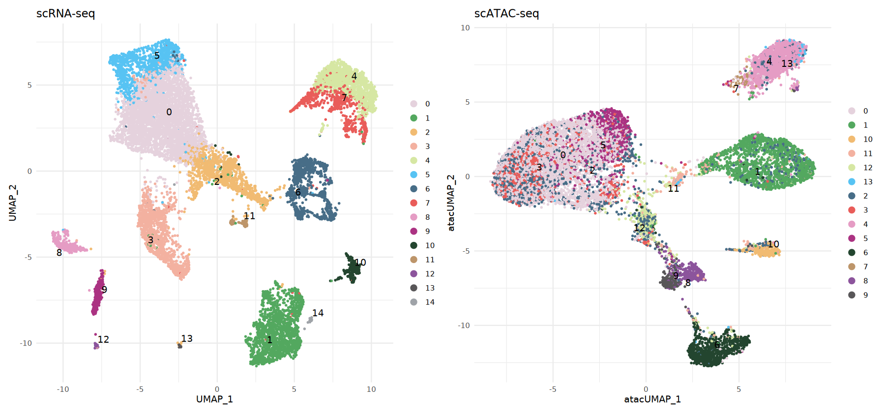
atac_obj <- AddMetaData(atac_obj, metadata = predicted.labels)

Visualize scATAC-seq cell types

Here we display side-by-side:

• RNA: cluster assignments present in or computed from the reference data
• ATAC: predicted cell types using label transfer (predicted.id)

Using the same color scheme for both makes it easy to directly compare the consistency between the two structures.

# scRNA-seq data visualization
options(repr.plot.width = 15, repr.plot.height = 7)
p1 <- DimPlot(rna_obj, 
              group.by = 'seurat_clusters', 
              label = TRUE, 
              repel = TRUE,
              pt.size = 0.5) + 
      ggtitle('scRNA-seq') +
      theme_minimal() +
      scale_color_manual(values = my36colors)

# scATAC-seq data visualization (based on predicted labels)

p2 <- DimPlot(atac_obj, 
              group.by = 'predicted.id', 
              label = TRUE, 
              repel = TRUE,
              pt.size = 0.5) + 
      ggtitle('scATAC-seq') +
      theme_minimal() +
      scale_color_manual(values = my36colors)
p1 | p2
pdf("scRNA_scATAC_UMAP.pdf", width = 10, height = 5)
print(p1 | p2)
dev.off()

pdf: 2

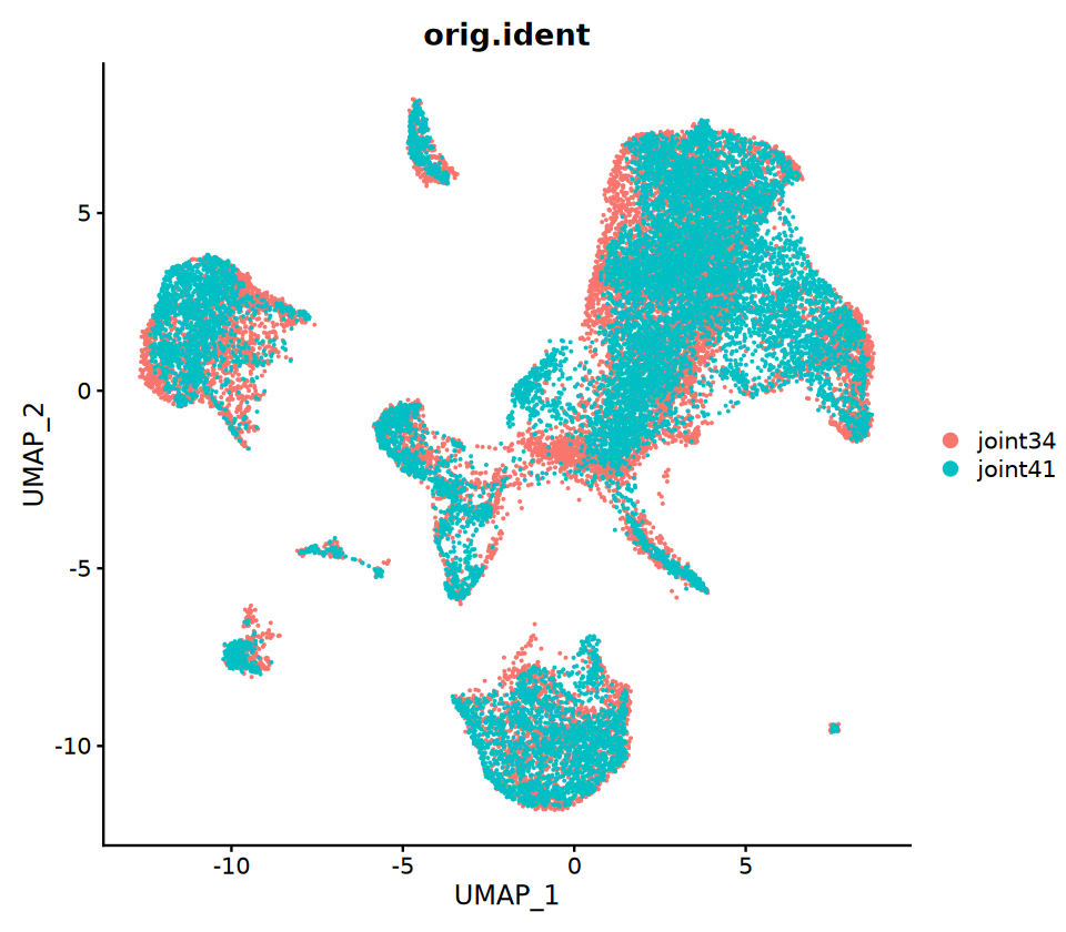
5. Co-embedding Analysis (Optional)

Purpose: Place both RNA and ATAC cells on the same UMAP plot to facilitate observation of cross-modality consistency. Key steps:

• First, use anchors to "impute/project" the RNA expression matrix onto the ATAC cells to obtain the "imputed expression matrix" for ATAC cells
• Next, merge both datasets and perform unified dimensionality reduction and UMAP visualization

Note: Co-embedding is mainly a visualization tool; it does not represent actual multi-omics measurements from the same cell. Interpret these results with biological context in mind.

# Compute co-embedding
suppressWarnings({
  suppressMessages({
      genes.use <- VariableFeatures(rna_obj)
      refdata <- GetAssayData(rna_obj, assay = "RNA", slot = "data")[genes.use, ]

# refdata (input) contains a scRNA-seq expression matrix for the scRNA-seq cells.  imputation
# (output) will contain an imputed scRNA-seq matrix for each of the ATAC cells
     imputation <- TransferData(anchorset = transfer.anchors, refdata = refdata, weight.reduction = "cca",dims=1:30)
     atac_obj[["RNA"]] <- imputation
     coembed <- merge(x = rna_obj, y = atac_obj)

     coembed <- ScaleData(coembed, features = genes.use, do.scale = FALSE)
     coembed <- RunPCA(coembed, features = genes.use, verbose = FALSE)
     coembed <- RunUMAP(coembed, dims = 1:30)
  })
})
options(repr.plot.width = 8, repr.plot.height = 7)
p3=DimPlot(coembed, group.by = c("orig.ident"))
p3
pdf("coembed_UMAP.pdf", width = 10, height = 5)
print(p3)
dev.off()

pdf: 2

6. Results Summary and Saving

After finishing, please save the key objects to facilitate reproducibility and downstream analysis:

• scRNA_processed.rds: The RNA object that has been normalized, reduced, and clustered
• scATAC_processed.rds: The ATAC object that has been quality-controlled, normalized, and labeled (including ACTIVITY)
• coembed.rds: The co-embedding object (if this step was performed)
• session_info.txt: Session environment information to help others reproduce your results

# Save analysis objects
saveRDS(rna_obj, file = "./scRNA_processed.rds")
saveRDS(atac_obj, file = "./scATAC_processed.rds")
saveRDS(coembed, file = "./coembed.rds")

7. Advanced Analysis Recommendations

After completing the basic integration, you may further explore the following analyses:

7.1 Transcription Factor Motif Analysis

• Use FindMotifs() to identify enriched TF motifs in differentially accessible regions (DAR)
• Infer changes in TF activity by combining RNA expression or gene activity data

7.2 Gene Regulatory Networks (GRN) and Peaks-to-Gene Linking

• Use LinkPeaks() to identify potential regulatory links between peaks and target genes
• If only single modality data are available, consider imputation or pseudo-bulk to associate expression with accessibility; ideally, use multi-omic data from the same cell for direct validation

7.3 Developmental Trajectory / Pseudotime Analysis

• Infer cellular trajectories within the integrated space
• Compare the dynamics of gene expression and chromatin accessibility along the trajectory

7.4 Differential Accessibility and Differential Expression

• Compare differential peaks and differential genes across different cell types or states
• Identify cell type-specific regulatory elements

7.5 Functional Enrichment

• Perform GO/KEGG enrichment analysis on differentially expressed genes or genes associated with differential peaks
• Interpret cellular functional characteristics using known pathways