scATAC-seq Multi-Sample Integration Tutorial (Signac / LSI)

Author: SeekGene

Time: 24 min

Words: 4.8k words

Updated: 2026-02-28

Reads: 0 times

scATAC + RNA-seq Analysis Guide Notebooks Basic Analysis

Environment Preparation

Loading R Packages

Please select the common_r environment for this integration tutorial

# Load necessary R packages
suppressPackageStartupMessages({
  library(Seurat)
  library(Signac)
  library(EnsDb.Hsapiens.v86, lib.loc = "/PROJ2/FLOAT/shumeng/apps/miniconda3/envs/python3.10/lib/R/library")
  library(BSgenome.Hsapiens.UCSC.hg38,lib = "/PROJ2/FLOAT/shumeng/apps/miniconda3/envs/python3.10/lib/R/library")
  library(biovizBase, lib = "/PROJ2/FLOAT/shumeng/apps/miniconda3/envs/python3.10/lib/R/library")
  #library(BSgenome.Mmusculus.UCSC.mm10)
  #library(EnsDb.Mmusculus.v79)
  library(dplyr)
  library(ggplot2)
  library(patchwork)
  library(harmony)
})

# Set random seed
set.seed(1234)

# Note, if data is large, you can customize resource settings
options(future.globals.maxSize = 15 * 1024^3)  # 15GB

my36colors <-c( '#E5D2DD', '#53A85F', '#F1BB72', '#F3B1A0', '#D6E7A3', '#57C3F3', '#476D87',
                '#E95C59', '#E59CC4', '#AB3282', '#23452F', '#BD956A', '#8C549C', '#585658',
                '#9FA3A8', '#E0D4CA', '#5F3D69', '#C5DEBA', '#58A4C3', '#E4C755', '#F7F398',
                '#AA9A59', '#E63863', '#E39A35', '#C1E6F3', '#6778AE', '#91D0BE', '#B53E2B',
                '#712820', '#DCC1DD', '#CCE0F5', '#CCC9E6', '#625D9E', '#68A180', '#3A6963',
                '#968175', "#6495ED", "#FFC1C1",'#f1ac9d','#f06966','#dee2d1','#6abe83','#39BAE8','#B9EDF8','#221a12',
                '#b8d00a','#74828F','#96C0CE','#E95D22','#017890')

Get Gene Annotation Information

We will obtain genomic annotation information (gene locations, transcripts, exons, TSS, etc.) for the corresponding species from the EnsDb database. The specific species needs to be changed according to the data. This information is used for:

• Calculate TSS Enrichment for ATAC (Judge if open chromatin is more concentrated near Transcription Start Sites)
• Building Gene Activity Matrix (Mapping peaks signals to genes)
• Peak Annotation and Functional Analysis

Notes:

• Species matches reference genome version (e.g., EnsDb.Hsapiens.v86 for hg38, EnsDb.Mmusculus.v75 for mm10)
• Consistent chromosome naming style (e.g., using chr1, chr2 prefixes)

# This tutorial uses human data, so we get gene annotation information
suppressWarnings({
  suppressMessages({
    annotation <- GetGRangesFromEnsDb(ensdb = EnsDb.Hsapiens.v86)
    seqlevels(annotation) <- paste0('chr', seqlevels(annotation))
    genome(annotation) <- 'hg38'
  })
})

# Set parallel computing (silent processing, optional)
suppressPackageStartupMessages({
  library(future)
})
plan("multicore", workers = 4)

Data Reading

This tutorial provides two different forms of data input to meet the data acquisition needs of different users. Just choose the one that suits you:

Cloud Platform RDS File Reading

Data Characteristics:

• RDS file is a standard Seurat object file
• Data has been preprocessed and multiple samples merged
• Can be directly used for subsequent downstream analysis, or extraction of expression matrices for reintegration

Applicable Scenarios:

• When you cannot obtain the standard filtered_peaks_bc_matrix expression matrix and fragment matrix
• When you want to integrate existing cloud platform data for learning
• When you need to quickly re-perform scRNA-seq data integration analysis

Notes:

• For specific data mounting and RDS file reading, please refer to the Jupyter usage tutorial

For example, the following project data /home/demo-SeekGene-com/workspace/data/AY1752565399550/

library(Seurat)
library(Signac)

# 1. Read Data
input <- readRDS("/home/demo-seekgene-com/workspace/data/AY1752565399550/input.rds")
meta <- read.table("/home/demo-seekgene-com/workspace/data/AY1752565399550/meta.tsv", 
                  header = TRUE, 
                  sep = "\t", 
                  row.names = 1)

# 2. Extract ATAC data and genome annotation
counts <- input@assays$ATAC@counts       # ATAC count matrix
fragments <- input@assays$ATAC@fragments # Fragment file (if available)
annotations <- input@assays$ATAC@annotation  # Genome annotation

# 3. Create ChromatinAssay (Signac format ATAC data)
atac_assay <- CreateChromatinAssay(
    counts = counts,
    fragments = fragments,
    annotation = annotations
)

# 4. Create Seurat object (containing only ATAC data)
atac_seurat <- CreateSeuratObject(
    counts = atac_assay,      # Use ChromatinAssay as input
    assay = "ATAC",          # Specify assay name
    meta.data = meta          # Add sample metadata
)

seurat_list <- SplitObject(atac_seurat, split.by = "Sample")

# 6. Clean up memory
rm(input, counts, fragments, annotations, atac_assay)
gc()

Standard filtered_peaks_bc_matrix File Reading

Applicable Scenarios:

• When you have standard gene expression matrices and peaks open matrix files
• When you want to independently complete multi-sample integration and batch correction of single-cell multi-omics (SeekArc) data
• When a complete workflow from raw data to integration analysis is needed

Note:

• Please ensure the file structure between samples is as follows:

The data directory structure must meet the following requirements:

1. The folder name for each sample is the Sample ID, such as S127, S44R, etc.
2. Each sample folder contains the following files:
   • filtered_peaks_bc_matrix: ATAC peak open matrix folder, containing barcodes.tsv.gz, features.tsv.gz, and matrix.mtx.gz files.
   • {Sample ID}_A_fragments.tsv.gz: ATAC fragments file, such as S127_A_fragments.tsv.gz.
   • {Sample ID}_A_fragments.tsv.gz.tbi: ATAC fragments index file, such as S127_A_fragments.tsv.gz.tbi.

The specific folder structure is as follows:

scATAC-seq Data (Peaks Matrix + Fragments)
├── S127/
│ ├── filtered_peaks_bc_matrix/
│ │ ├── barcodes.tsv.gz (Cell barcodes)
│ │ ├── features.tsv.gz (Peaks list)
│ │ └── matrix.mtx.gz (Sparse count matrix)
│ ├── S127_A_fragments.tsv.gz (Genomic coordinates of each sequencing read)
│ ├── S127_A_fragments.tsv.gz.tbi (Index file for fragments)
│ └── per_barcode_metrics.csv (Optional, per-cell QC metrics)
├── S44R/
│ ├── filtered_peaks_bc_matrix/
│ │ ├── barcodes.tsv.gz
│ │ ├── features.tsv.gz
│ │ └── matrix.mtx.gz
│ ├── S44R_A_fragments.tsv.gz
│ ├── S44R_A_fragments.tsv.gz.tbi
│ └── per_barcode_metrics.csv (optional)

# Define sample names
sample_names <- c('S127', 'S44R')
# Create an empty list to store the Seurat object for each sample
seurat_list <- list()

for (sample in sample_names) {
  cat('Processing sample:', sample, '\n')
  
  # Construct file paths
  counts_path <- file.path(sample, 'filtered_peaks_bc_matrix')
  fragments_path <- file.path(sample, paste0(sample, '_A_fragments.tsv.gz'))
  #metadata_path <- file.path(sample, 'per_barcode_metrics.csv')
  
  # Read peaks matrix data
  counts <- Read10X(counts_path)
  
  # Read QC metrics metadata
  #metadata <- read.csv(
  #  file = metadata_path,
  #  header = TRUE,
  #  row.names = 1
  #)
  
  # Creating ChromatinAssay object
  chrom_assay <- CreateChromatinAssay(
    counts = counts,
    sep = c(":", "-"),
    fragments = fragments_path,
    min.cells = 3,
    min.features = 200
  )
  
  # Create Seurat object
  obj <- CreateSeuratObject(
    counts = chrom_assay,
    assay = "ATAC"#,meta.data = metadata
  )
  
  # Add gene annotation information
  Annotation(obj) <- annotation
  
  # Add sample ID
  obj$Sample <- sample
  obj$orig.ident <- sample
  
  # Adding Seurat object to list
  seurat_list[[sample]] <- obj
  
  cat('Sample', sample, 'processed, cell count:', ncol(obj), '\n')
}

Quality Control

QC Metrics Calculation

Common scATAC-seq QC metrics:

• TSS.enrichment (TSS Enrichment Score, usually > 2): Higher is better, indicating signals are more concentrated near transcription start sites; too low may indicate high background or poor cell viability.
• nucleosome_signal (Nucleosome Signal, lower is better): Reflects nucleosome periodicity signal; usually lower is better.
• blacklist_ratio (Blacklist Ratio): Proportion of reads falling into genomic blacklist regions; too high indicates data quality issues.
• nCount_ATAC: Total ATAC counts; extremely low or high values require caution.

Actual thresholds should be set based on data distribution and judged in combination with fragments quality, doublet ratios, etc.

# Quality control for each sample
suppressWarnings({
  suppressMessages({
      for (sample_name in names(seurat_list)) {
      seurat_obj <- seurat_list[[sample_name]]
  
      # Set default assay to ATAC
      DefaultAssay(seurat_obj) <- 'ATAC'
      # Calculate TSS enrichment score
      seurat_obj <- TSSEnrichment(seurat_obj)
      # Calculate nucleosome signal
      seurat_obj <- NucleosomeSignal(seurat_obj)
      # Calculate blacklist region read ratio
      seurat_obj$blacklist_ratio <- FractionCountsInRegion(
        object = seurat_obj,
        assay = 'ATAC',
        regions = blacklist_hg38_unified)
      # Update objects in seurat_list
      seurat_list[[sample_name]] <- seurat_obj
      }
  })
})

output

Extracting TSS positions

Extracting fragments at TSSs


Computing TSS enrichment score

Extracting TSS positions

Extracting fragments at TSSs


Computing TSS enrichment score

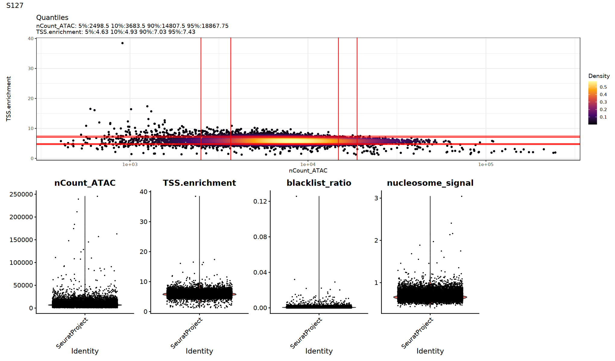
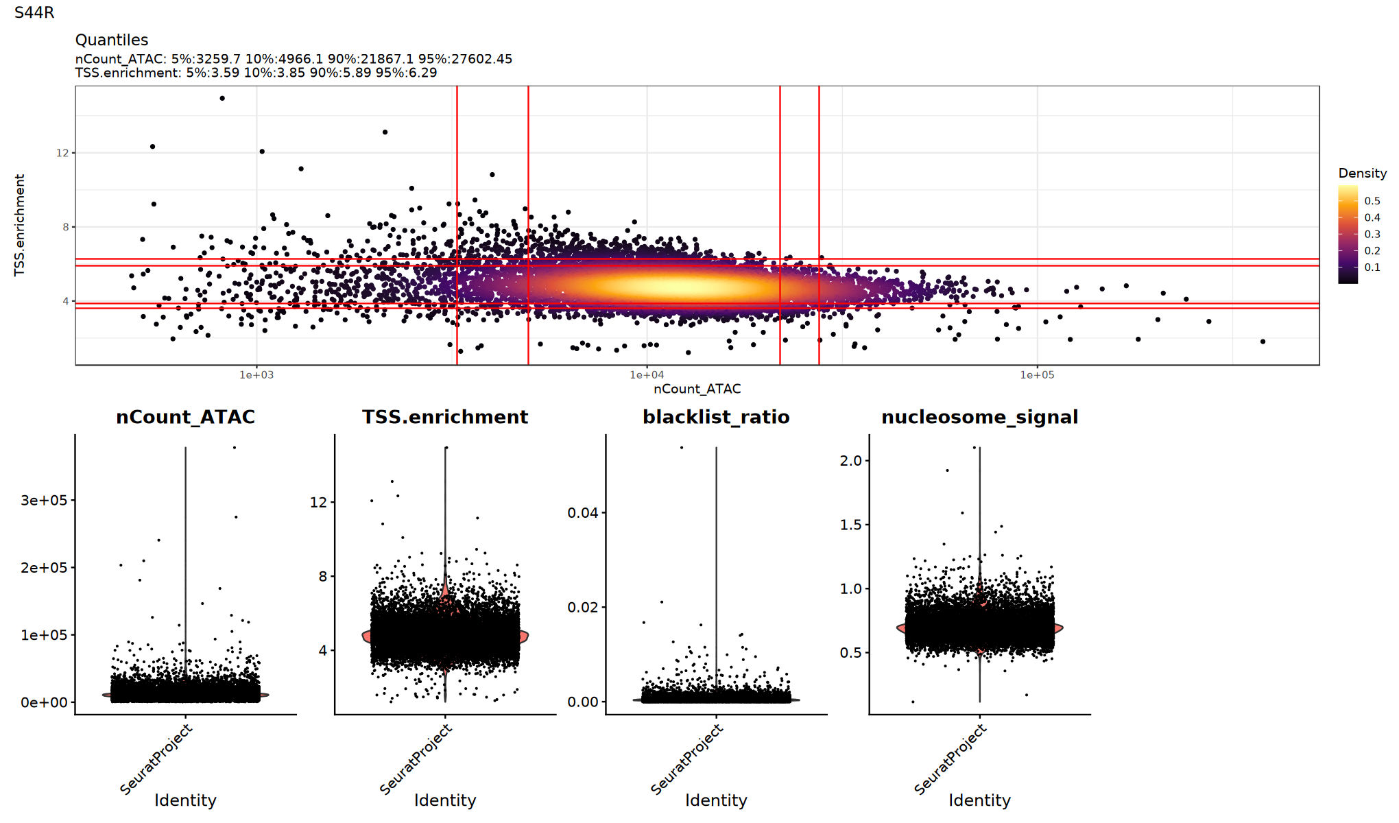
QC Metrics Visualization

Use violin plots to view the distribution/outliers of each QC metric to determine appropriate thresholds:

Suggestion:

• Observe whether there is an obvious long tail or bimodal distribution
• Try multiple thresholds and compare if downstream clustering/UMAP is clearer

# Visualize QC metrics (optional execution)
options(repr.plot.width = 17, repr.plot.height = 10)
suppressWarnings({
for (sample_name in names(seurat_list)) {
  seurat_obj <- seurat_list[[sample_name]]
  p1=DensityScatter(seurat_obj, x = 'nCount_ATAC', y = 'TSS.enrichment', log_x = TRUE, quantiles = TRUE)
  p2=VlnPlot(
      object = seurat_obj,
      features = c('nCount_ATAC', 'TSS.enrichment', 'blacklist_ratio', 'nucleosome_signal'),
      pt.size = 0.1,
      ncol = 5
  )
 print(p1 / p2 + plot_annotation(title = sample_name))
}
})

Low Quality Cell Filtering

Filter low-quality cells based on QC metrics. Specific thresholds should be adjusted according to data characteristics. Refer to the violin plot distribution above for specific filtering thresholds.

# Set QC filtering thresholds (adjust based on data characteristics)
for (sample_name in names(seurat_list)) {
  cat('Filtering sample', sample_name, '...\n')
  
  seurat_obj <- seurat_list[[sample_name]]
  
  # Record cell count before filtering
  cells_before <- ncol(seurat_obj)
  
  # Filter based on QC metrics
  seurat_obj <- subset(
    x = seurat_obj,
    subset = nCount_ATAC > 500 &
             nCount_ATAC  < 100000 &
             blacklist_ratio < 0.05 &
             nucleosome_signal < 2 &
             TSS.enrichment > 1
  )
  
  # Record cell count after filtering
  cells_after <- ncol(seurat_obj)
  
  # Update seurat_list
  seurat_list[[sample_name]] <- seurat_obj
  
  cat('Sample', sample_name, 'filtered: ', cells_before, ' cells before, ', cells_after, ' cells after\n')
}

output

正在对样本 S127 进行质控过滤...n 样本 S127 过滤完成: 过滤前 13946 个细胞，过滤后 13916 个细胞
正在对样本 S44R 进行质控过滤...n 样本 S44R 过滤完成: 过滤前 12068 个细胞，过滤后 12050 个细胞

Calculate Common Peaks Between Samples

Since peak calling is performed independently for each sample, the peaks in different samples are different. To integrate multiple samples, we need to unify peak information and create a common peak set for all samples.

Processing Workflow:

1. Merge peaks from all samples
2. Filter peak length (20bp-10kb)
3. Re-quantify common peaks for each sample

Notes: If the first method (reading RDS) was used to read data earlier, this part does not need to be analyzed.

Notes: If the first method (reading RDS) was used to read data earlier, this part does not need to be analyzed.

Notes: If the first method (reading RDS) was used to read data earlier, this part does not need to be analyzed.

# Extract peaks information for each sample
all_peaks <- lapply(seurat_list, function(x) {
  DefaultAssay(x) <- "ATAC"
  granges(x@assays$ATAC)
})

# Merge peaks from all samples
gr_list <- GRangesList(all_peaks)
all_granges <- unlist(gr_list, use.names = FALSE)
combined.peaks <- reduce(x = all_granges)

# Filter peak length (keep 20bp-10kb peaks)
peakwidths <- width(combined.peaks)
common_peaks <- combined.peaks[peakwidths < 10000 & peakwidths > 20]

cat('Total peaks count:', length(common_peaks), '\n')

# Quantify common peaks for each sample
seurat_list <- lapply(seurat_list, function(x) {
  cat('Quantifying common peaks for sample', x$Sample[1], '...\n')
  
  # Quantify counts matrix for common peaks
  combined_counts <- FeatureMatrix(
    fragments = Fragments(x@assays$ATAC),
    features = common_peaks,
    cells = colnames(x)
  )
  
  # Create new ChromatinAssay
  combined_peaks_assay <- CreateChromatinAssay(
    counts = combined_counts,
    fragments = Fragments(x@assays$ATAC),
    annotation = Annotation(x@assays$ATAC)
  )
  
  # Add to Seurat object
  x[["combinedpeaks"]] <- combined_peaks_assay
  DefaultAssay(x) <- "combinedpeaks"
  x[["ATAC"]] <- NULL
  return(x)
})

output

共有peaks数量: 211924
正在为样本 S127 量化共有peaks...n

Extracting reads overlapping genomic regions



正在为样本 S44R 量化共有peaks...n

Extracting reads overlapping genomic regions

Multi-Sample Merging

In the multi-omics data integration analysis workflow, multi-sample merging is an important prerequisite step for integration analysis.

Purpose of Merging:

• Integrate data from multiple samples into a single Seurat object
• Prepare for subsequent batch correction and integration analysis
• Facilitate comparative analysis with batch-corrected results

Important Note:

• This step only performs simple data merging, batch effect correction has not been performed yet
• Merged object contains raw data from all samples
• Perform normalization, feature selection, PCA dimensionality reduction, and UMAP visualization on merged data

suppressWarnings({
  suppressMessages({
      # Merge scATAC-seq datasets
      obj.combined <- merge(seurat_list[[1]], seurat_list[-1], merge.data = FALSE)
      # Set default assay and normalize
      DefaultAssay(obj.combined) <- "combinedpeaks"
      obj.combined <- FindTopFeatures(obj.combined, min.cutoff = 10)
      obj.combined <- RunTFIDF(obj.combined)
      obj.combined <- RunSVD(obj.combined)
      obj.combined <- RunUMAP(obj.combined, reduction = "lsi", dims = 2:30,reduction.name="atacumap")
        })
})

Data Integration

Now we will integrate scATAC-seq data from multiple samples. There are two common methods for scATAC-seq data integration:

Integration Method Selection

CCA (Canonical Correlation Analysis) Integration:

• Integration method based on Canonical Correlation Analysis (CCA)
• Integrate by finding common variation patterns between samples
• Suitable for cases with large differences between samples
• Classic integration method in Seurat package

Harmony Integration:

• Fast integration method based on iterative clustering
• Correct batch effects directly in dimensionality reduction space
• High computational efficiency, suitable for large-scale data
• Retain more biological variation information

Method Selection Suggestions

• Harmony: scATAC-seq data from the same platform but different samples; Harmony is faster for large numbers of samples or large datasets.
• CCA: Runs longer, usually recommended when batch effects are severe, such as cross-platform scATAC-seq data.

Integration using Harmony

Note: Choose either Harmony or CCA for batch correction

atac_integrate_harmony <- function(obj) {
  library(harmony)
  DefaultAssay(obj) <- "combinedpeaks"
  obj<- RunHarmony(
        object = obj,
        group.by.vars = 'Sample',
        reduction = 'lsi',
        assay.use = 'combinepeaks',
        reduction.save = "harmonylsi",
        project.dim = FALSE
        )
  obj <- RunUMAP(obj,reduction = 'harmonylsi',reduction.name="atacharmonyumap", dims = 2:30)
  #obj <- RunTSNE(obj, reduction = "harmonylsi",reduction.name="atacharmonytsne",dims = 2:50,check_duplicates = FALSE)
  return(obj)
}
suppressWarnings({
  suppressMessages({
      integrated=atac_integrate_harmony(obj.combined)
      integrated <- FindNeighbors(object = integrated, reduction = 'harmonylsi', graph.name = "atacneighbor", dims = 2:30)
      integrated <- FindClusters(object = integrated, verbose = FALSE, graph.name = "atacneighbor",resolution = 0.5, algorithm = 3)
      
  })
})
# Visualize ATAC batch correction effect
options(repr.plot.width=10, repr.plot.height=8)
DimPlot(integrated, reduction = "atacharmonyumap", group.by = "Sample")

Integration using CCA

Note: Choose either Harmony or CCA for batch correction

# Define ATAC integration function
options(future.globals.maxSize = 20 * 1024^3)
integrate_atac_cca <- function(object.list){
    object.list <- lapply(object.list, function(x) {
        DefaultAssay(x)="combinedpeaks"
        x=RunTFIDF(x)
        x=FindTopFeatures(x, min.cutoff = 5)
        x=RunSVD(x)
        return(x)
      })
    
    anchors <- FindIntegrationAnchors(
        object.list = object.list,
        anchor.features = rownames(obj.combined),
        reduction = "rlsi",
        dims = 2:30
    )
    
    integrated <- IntegrateEmbeddings(
            anchorset = anchors,
            reductions = obj.combined[["lsi"]],
            new.reduction.name = "integrated_lsi",
            dims.to.integrate = 1:30)
   integrated<- RunUMAP(integrated, reduction = "integrated_lsi", dims = 2:30,reduction.name="atacintegratedumap")
   #integrated<- RunTSNE(integrated, reduction = "integrated_lsi", dims = 2:30,reduction.name="atacintegratedtsne")
   return(integrated)
}

# Execute ATAC integration
suppressWarnings({
  suppressMessages({
      integrated <- integrate_atac_cca(seurat_list)
      integrated <- FindNeighbors(object = integrated, reduction = 'integrated_lsi', graph.name = "atacneighbor", dims = 2:30)
      integrated <- FindClusters(object = integrated, verbose = FALSE, graph.name = "atacneighbor",resolution = 0.5, algorithm = 3)
  })
})  

# Visualize ATAC batch correction effect
options(repr.plot.width=10, repr.plot.height=8)
DimPlot(integrated, reduction = "atacintegratedumap", group.by = "Sample")

output

开始ATAC整合分析... 1754708454
开始处理各样本的LSI降维...n 寻找整合锚点...n 整合嵌入向量...

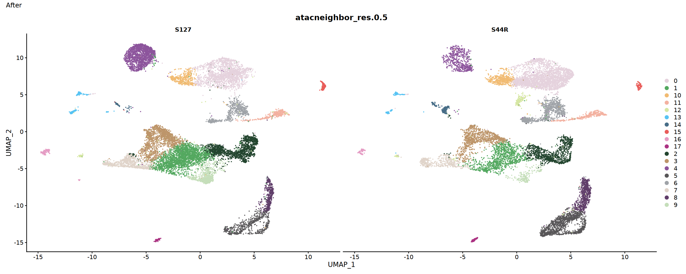
Integration Effect Assessment

Compare results before and after integration to assess integration effect.

Assessment Metrics:

• Sample mixing degree: Distribution of cells from different samples in UMAP plot
• Batch effect removal: Clustering of technical replicates
• Biological signal preservation: Separation of known cell types

suppressWarnings({
  suppressMessages({
      # Create control data before integration
      obj.combined <- FindNeighbors(object = obj.combined, 
                                 reduction = 'lsi', 
                                 graph.name = "atacneighbor", 
                                 dims = 2:30)
      # Cluster Analysis
      obj.combined <- FindClusters(object = obj.combined, 
                                verbose = FALSE, 
                                graph.name = "atacneighbor", 
                                cluster.name = "atac_clusters", 
                                resolution = 0.5, 
                                algorithm = 3)
  })
})

options(repr.plot.width=15, repr.plot.height=6)
# Sample distribution before integration
p1 <- DimPlot(obj.combined, split.by = "Sample" , cols = my36colors)+plot_annotation(title = "Before")

# Sample distribution after integration. Select the reduction parameter below according to the integration method used previously
p2 <- DimPlot(integrated, split.by = "Sample" , cols = my36colors, reduction = "atacharmonyumap" ,group.by = "atacneighbor_res.0.5")+plot_annotation(title = "After")
#p2 <- DimPlot(integrated, split.by = "Sample" , cols = my36colors, reduction = "atacintegratedumap",group.by = "atacneighbor_res.0.5")+plot_annotation(title = "After")
p1
p2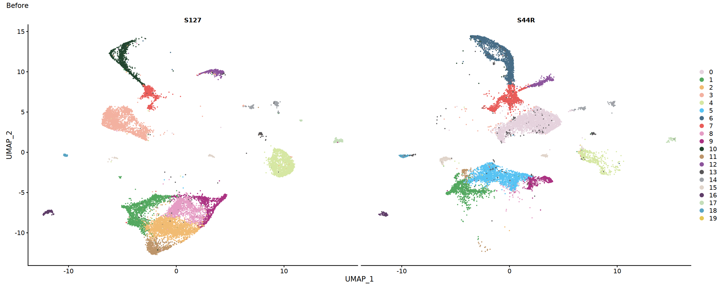

Cell Annotation

Cell type annotation based on gene activity scores, identifying different cell types through known marker genes. Gene activity can only roughly classify scATAC-seq data. Specific annotation strategies for scATAC-seq data include:
(1) Rough classification using gene activity;
(2) Using annotated scRNA-seq of the same tissue as a reference to transfer scRNA-seq cell labels to scATAC-seq to complete cell annotation;
(3) Using CoveragePlot in the Signac package to visualize the specific opening of marker gene peaks to complete cell annotation. This tutorial only demonstrates cell annotation using marker gene activity.

Gene Activity Analysis

Principle: Count peaks signals associated with each gene (e.g., gene body + promoter region within a certain range upstream/downstream) and accumulate them to obtain the "activity score" of that gene in each cell.

• Typical practice takes ~2kb upstream and ~1kb downstream of TSS (adjustable)
• The resulting ACTIVITY assay will be used to build anchors with RNA assay

# Calculate gene activity score
gene.activities <- GeneActivity(integrated)

# Add gene activity matrix as a new assay
integrated[['RNA']] <- CreateAssayObject(counts = gene.activities)
DefaultAssay(integrated)="RNA"
# Normalize gene activity data
integrated <- NormalizeData(
  object = integrated,
  assay = 'RNA',
  normalization.method = 'LogNormalize',
  scale.factor = median(integrated$nCount_RNA)
)

output

Extracting gene coordinates

Extracting reads overlapping genomic regions

Extracting reads overlapping genomic regions

Collect Typical Marker Genes for Cell Types

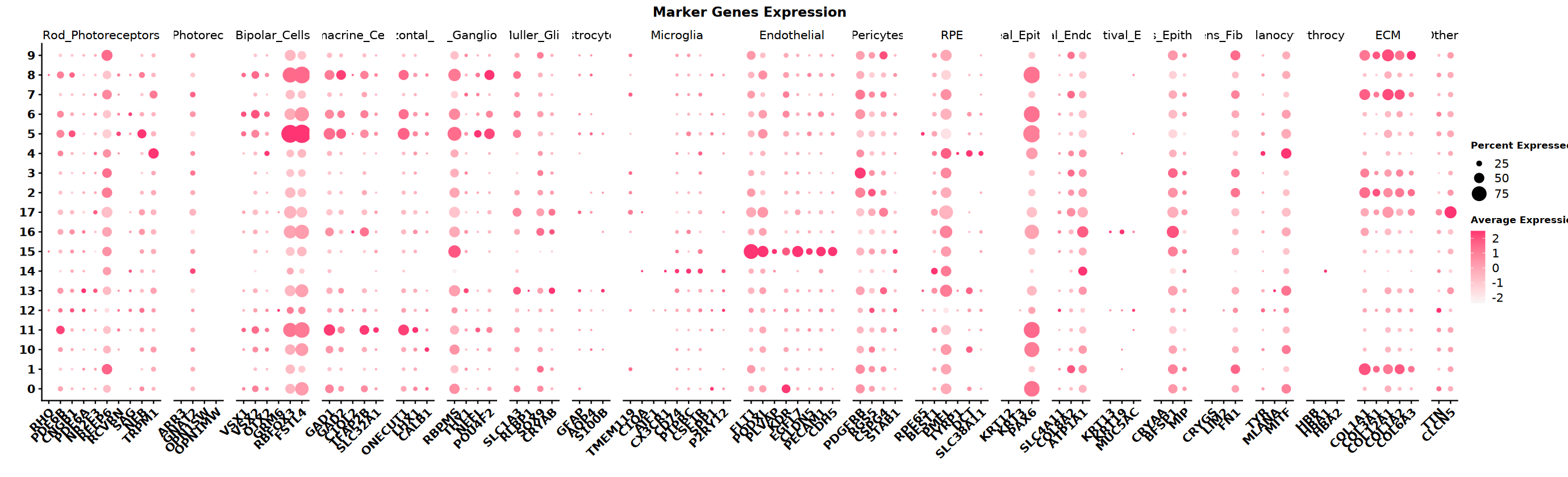
Collect marker gene sets for different cell types based on tissue type. This example data is from the eye. Below are the cell types in the eye and their corresponding marker genes. Use a dot plot to visualize which cell types' marker genes are highly open in different clusters.

eye_marker_integrated <- list(
  # ========== Photoreceptor Cells ==========
  "Rod_Photoreceptors" = c("RHO", "PDE6B", "CNGB1", "PDE6A", "NR2E3", "REEP6",
                          "RCVRN", "SAG", "NEB", "SLC24A3", "TRPM1"),
  "Cone_Photoreceptors" = c("ARR3", "GNAT2", "OPN1SW", "OPN1MW", "TRPM3"),

  # ========== Retinal Neurons ==========
  "Bipolar_Cells" = c("VSX1", "VSX2", "OTX2", "GRM6", "PRKCA",
                     "DLG2", "NRXN3", "RBFOX3", "FSTL4"),
  "Amacrine_Cells" = c("GAD1", "GAD2", "C1QL2", "TFAP2B", "SLC32A1"),
  "Horizontal_Cells" = c("ONECUT1", "LHX1", "CALB1", "NFIA"),
  "Retinal_Ganglion_Cells" = c("RBPMS", "THY1", "NEFL", "POU4F2"),

  # ========== Glial Cells ==========
  "Muller_Glia" = c("SLC1A3", "RLBP1", "SOX9", "CRYAB"),
  "Astrocytes" = c("GFAP", "AQP4", "S100B"),
  "Microglia" = c("TMEM119", "C1QA", "AIF1", "CX3CR1", "CD74",
                 "PTPRC", "CSF1R", "CCL3L1", "SPP1", "P2RY12"),

  # ========== Vascular and Support Cells ==========
  "Endothelial" = c("FLT1", "PODXL", "PLVAP", "KDR", "EGFL7",
                   "CLDN5", "PECAM1", "CDH5"),
  "Pericytes" = c("PDGFRB", "RGS5", "CSPG4", "STAB1"),

  # ========== Epithelial Cells ==========
  "RPE" = c("RPE65", "BEST1", "PMEL", "TYRP1", "DCT", "SLC38A11"),
  "Corneal_Epithelial" = c("KRT12", "KRT3", "PAX6"),
  "Corneal_Endothelial" = c("SLC4A11", "COL8A2", "ATP1A1"),
  "Conjunctival_Epithelial" = c("KRT13", "KRT19", "MUC5AC"),

  # ========== Lens Cells ==========
  "Lens_Epithelial" = c("CRYAA", "BFSP1", "MIP"),
  "Lens_Fiber" = c("CRYGS", "LIM2", "FN1"),

  # ========== Other Cells ==========
  "Melanocytes" = c("TYR", "MLANA", "MITF"),
  "Erythrocytes" = c("HBB", "HBA1", "HBA2"),
  "ECM" = c("COL1A1", "COL3A1", "COL12A1", "COL1A2", "COL6A3"),
  "Others" = c("TTN", "CLCN5", "DCC", "MIAT")
)

# Set plot size
options(repr.plot.width=23, repr.plot.height=7)

# Draw DotPlot
DotPlot(integrated, 
        group.by = "atacneighbor_res.0.5", 
        features = eye_marker_integrated,
        cols = c("#f8f8f8","#ff3472"),
       dot.min = 0.05,
       dot.scale = 8)+  # Apply custom color scheme
  RotatedAxis() + 
  scale_x_discrete("") + 
  scale_y_discrete("") +
  theme(
    axis.text.x = element_text(size = 12, face = "bold", 
                              angle = 45, hjust = 1, vjust = 1),
    axis.text.y = element_text(size = 12, face = "bold"),
    plot.title = element_text(size = 14, face = "bold", hjust = 0.5),
    legend.title = element_text(size = 10, face = "bold")
  ) +
  ggtitle("Marker Genes Expression") +
  labs(color = "Expression\nLevel")  # Modify legend title

output

Warning message in FetchData.Seurat(object = object, vars = features, cells = cells):
"The following requested variables were not found: SLC24A3, TRPM3, PRKCA, DLG2, NRXN3, NFIA, CCL3L1, DCC, MIAT"

Warning message:
"Removed 530 rows containing missing values or values outside the scale range
(\`geom_point()\`)."

Cell Type Labeling

Assign cell type labels to each cluster based on marker gene opening patterns (i.e., gene activity status).

# Define cell types based on clustering results and marker gene expression
# Note: The specific mapping from clusters to cell types needs to be adjusted based on marker gene expression results
integrated$celltype <- recode(integrated$atacneighbor_res.0.5,
                                   "0"  = "Photoreceptors",
                                   "1"  = "ECM",
                                   "2"  = "ECM",
                                   "3"  = "ECM",
                                   "4"  = "Rod_photoreceptors",
                                   "5"  = "Bipolar_Cells",
                                   "6"  = "Amacrine_Horizontal",
                                   "7"  = "ECM",
                                   "8"  = "Bipolar_Cells",
                                   "9"  = "ECM",
                                   "10" = "Photoreceptors",
                                   "11" = "Amacrine_Horizontal",
                                   "12" = "Photoreceptors",
                                   "13" = "Muller_Glia",
                                   "14" = "Microglia",
                                   "15" = "Endothelial",
                                   "16" = "Muller_Glia",
                                   "17" = "ECM"
 )

# Basic UMAP plot
p1 <- DimPlot(integrated, 
             cols = my36colors, 
             group.by = "celltype", 
             label = TRUE) +
  ggtitle("Cell Type Annotation")

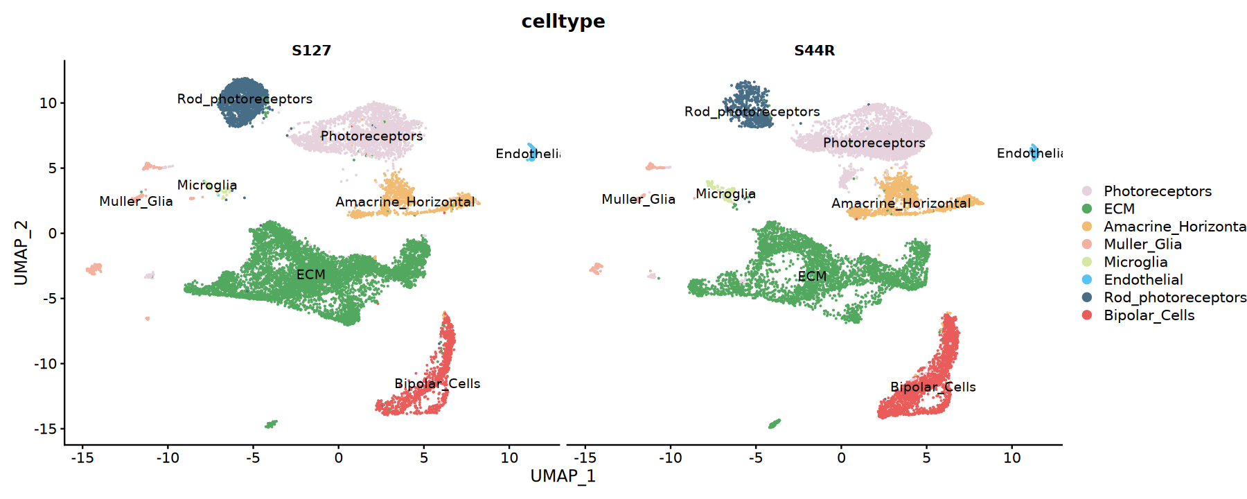
# Split sample UMAP plot
p2 <- DimPlot(integrated, 
             cols = my36colors, 
             split.by = "Sample",
             group.by = "celltype", 
             label = TRUE)

# Save PDF (high quality vector graphic)
ggsave('./celltype_annotation_umap.pdf', p1, width = 8, height = 6)
ggsave('./celltype_by_sample_umap.pdf', p2, width = 16, height = 6)

# Display graphics
# Set plot dimensions
options(repr.plot.width=9, repr.plot.height=6)
print(p1)
# Set plot dimensions
options(repr.plot.width=15, repr.plot.height=6)
print(p2)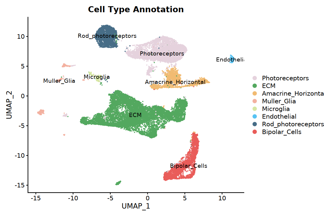

Save Results

Save the integrated object and key charts. It is recommended to save intermediate objects at the same time for reproduction and subsequent review.

saveRDS(integrated, file = "./integrated.rds")

Summary

This tutorial demonstrates the complete workflow for scATAC-seq multi-sample integration analysis:

Key Technical Points

• TF-IDF Normalization: Suitable for sparse scATAC-seq data
• LSI Dimensionality Reduction: Latent Semantic Indexing, more suitable for scATAC-seq data than PCA
• Peaks Merging: Unifying peak sets from different samples is a key step in integration
• Gene Activity Score: Convert peaks signals to gene-level activity scores

Notes

• QC Thresholds: Filtering parameters need to be adjusted based on specific data characteristics
• Integration Parameters: LSI dimension selection and integration parameters need optimization
• Cell Annotation: Manual annotation requires combining biological knowledge and marker gene expression
• Computational Resources: scATAC-seq data volume is large and requires sufficient memory and computational resources

Suggestions for Subsequent Analysis

• Differential Accessibility Region (DAR) Analysis
• Transcription Factor Footprint Analysis
• Gene Regulatory Network Inference
• Multi-omics Integration Analysis with scRNA-seq Data
• Cell Trajectory and Pseudotime Analysis

sessionInfo()

output

R version 4.3.3 (2024-02-29)
Platform: x86_64-conda-linux-gnu (64-bit)
Running under: Debian GNU/Linux 12 (bookworm)

Matrix products: default
BLAS/LAPACK: /jp_envs/envs/common/lib/libopenblasp-r0.3.29.so; LAPACK version 3.12.0

locale:
[1] LC_CTYPE=C.UTF-8 LC_NUMERIC=C LC_TIME=C.UTF-8
[4] LC_COLLATE=C.UTF-8 LC_MONETARY=C.UTF-8 LC_MESSAGES=C.UTF-8
[7] LC_PAPER=C.UTF-8 LC_NAME=C LC_ADDRESS=C
[10] LC_TELEPHONE=C LC_MEASUREMENT=C.UTF-8 LC_IDENTIFICATION=C

time zone: Asia/Shanghai
tzcode source: system (glibc)

attached base packages:
[1] stats4 stats graphics grDevices utils datasets methods
[8] base

other attached packages:
[1] future_1.40.0 patchwork_1.3.0
[3] ggplot2_3.5.2 dplyr_1.1.4
[5] biovizBase_1.50.0 BSgenome.Hsapiens.UCSC.hg38_1.4.5
[7] BSgenome_1.70.1 rtracklayer_1.62.0
[9] BiocIO_1.12.0 Biostrings_2.70.1
[11] XVector_0.42.0 EnsDb.Hsapiens.v86_2.99.0
[13] ensembldb_2.26.0 AnnotationFilter_1.26.0
[15] GenomicFeatures_1.54.1 AnnotationDbi_1.64.1
[17] Biobase_2.62.0 GenomicRanges_1.54.1
[19] GenomeInfoDb_1.38.1 IRanges_2.36.0
[21] S4Vectors_0.40.2 BiocGenerics_0.48.1
[23] Signac_1.10.0 SeuratObject_4.1.4
[25] Seurat_4.4.0 repr_1.1.7

loaded via a namespace (and not attached):
[1] ProtGenerics_1.34.0 matrixStats_1.5.0
[3] spatstat.sparse_3.1-0 bitops_1.0-9
[5] httr_1.4.7 RColorBrewer_1.1-3
[7] tools_4.3.3 sctransform_0.4.1
[9] backports_1.5.0 R6_2.6.1
[11] lazyeval_0.2.2 uwot_0.2.3
[13] withr_3.0.2 sp_2.2-0
[15] prettyunits_1.2.0 gridExtra_2.3
[17] progressr_0.15.1 cli_3.6.4
[19] Cairo_1.6-2 spatstat.explore_3.4-2
[21] labeling_0.4.3 spatstat.data_3.1-6
[23] ggridges_0.5.6 pbapply_1.7-2
[25] Rsamtools_2.18.0 pbdZMQ_0.3-13
[27] foreign_0.8-87 R.utils_2.13.0
[29] dichromat_2.0-0.1 parallelly_1.43.0
[31] rstudioapi_0.15.0 RSQLite_2.3.9
[33] generics_0.1.3 ica_1.0-3
[35] spatstat.random_3.3-3 Matrix_1.6-5
[37] ggbeeswarm_0.7.2 abind_1.4-5
[39] R.methodsS3_1.8.2 lifecycle_1.0.4
[41] yaml_2.3.10 SummarizedExperiment_1.32.0
[43] SparseArray_1.2.2 BiocFileCache_2.10.1
[45] Rtsne_0.17 grid_4.3.3
[47] blob_1.2.4 promises_1.3.2
[49] crayon_1.5.3 miniUI_0.1.1.1
[51] lattice_0.22-7 cowplot_1.1.3
[53] KEGGREST_1.42.0 pillar_1.10.2
[55] knitr_1.49 rjson_0.2.23
[57] future.apply_1.11.3 codetools_0.2-20
[59] fastmatch_1.1-6 leiden_0.4.3.1
[61] glue_1.8.0 spatstat.univar_3.1-2
[63] data.table_1.17.0 vctrs_0.6.5
[65] png_0.1-8 gtable_0.3.6
[67] cachem_1.1.0 xfun_0.50
[69] S4Arrays_1.2.0 mime_0.13
[71] survival_3.8-3 RcppRoll_0.3.1
[73] fitdistrplus_1.2-2 ROCR_1.0-11
[75] nlme_3.1-168 bit64_4.5.2
[77] progress_1.2.3 filelock_1.0.3
[79] RcppAnnoy_0.0.22 irlba_2.3.5.1
[81] vipor_0.4.7 KernSmooth_2.23-26
[83] rpart_4.1.23 colorspace_2.1-1
[85] DBI_1.2.3 Hmisc_5.2-1
[87] nnet_7.3-19 ggrastr_1.0.2
[89] tidyselect_1.2.1 bit_4.5.0.1
[91] compiler_4.3.3 curl_6.0.1
[93] htmlTable_2.4.3 xml2_1.3.6
[95] DelayedArray_0.28.0 plotly_4.10.4
[97] checkmate_2.3.2 scales_1.3.0
[99] lmtest_0.9-40 rappdirs_0.3.3
[101] stringr_1.5.1 digest_0.6.37
[103] goftest_1.2-3 spatstat.utils_3.1-3
[105] rmarkdown_2.29 htmltools_0.5.8.1
[107] pkgconfig_2.0.3 base64enc_0.1-3
[109] MatrixGenerics_1.14.0 dbplyr_2.5.0
[111] fastmap_1.2.0 rlang_1.1.5
[113] htmlwidgets_1.6.4 shiny_1.10.0
[115] farver_2.1.2 zoo_1.8-14
[117] jsonlite_2.0.0 BiocParallel_1.36.0
[119] R.oo_1.27.0 VariantAnnotation_1.48.1
[121] RCurl_1.98-1.16 magrittr_2.0.3
[123] Formula_1.2-5 GenomeInfoDbData_1.2.11
[125] IRkernel_1.3.2 munsell_0.5.1
[127] Rcpp_1.0.14 reticulate_1.42.0
[129] stringi_1.8.7 zlibbioc_1.48.0
[131] MASS_7.3-60.0.1 plyr_1.8.9
[133] parallel_4.3.3 listenv_0.9.1
[135] ggrepel_0.9.6 deldir_2.0-4
[137] IRdisplay_1.1 splines_4.3.3
[139] tensor_1.5 hms_1.1.3
[141] igraph_2.0.3 uuid_1.2-1
[143] spatstat.geom_3.3-6 reshape2_1.4.4
[145] biomaRt_2.58.0 XML_3.99-0.17
[147] evaluate_1.0.3 httpuv_1.6.15
[149] RANN_2.6.2 tidyr_1.3.1
[151] purrr_1.0.4 polyclip_1.10-7
[153] scattermore_1.2 xtable_1.8-4
[155] restfulr_0.0.15 later_1.4.2
[157] viridisLite_0.4.2 tibble_3.2.1
[159] memoise_2.0.1 beeswarm_0.4.0
[161] GenomicAlignments_1.38.0 cluster_2.1.8.1
[163] globals_0.16.3