scMethyl + RNA Multi-omics: Basic Analysis Workflow

Author: SeekGene

Time: 50 min

Words: 10.3k words

Updated: 2026-02-28

Reads: 0 times

scMethyl + RNA-seq Notebooks

Module Introduction

This module is designed for basic analysis of single-cell methylation dual-omics data (containing both RNA and methylation information).

This module implements the following core analysis workflows:

• Data Integration: Integrates single-cell RNA-seq and single-cell methylation sequencing data from multiple samples.
• Quality Control: Perform independent quality control filtering on RNA and methylation data to ensure data quality.
• Batch Effect Correction: Uses Harmony algorithm to correct technical variations between multiple samples while preserving biological signals.
• Cell Atlas Construction: Constructs a single-cell atlas via dimensionality reduction, clustering, and visualization to identify cell types and subpopulations.

Input File Preparation

This module requires the following input files:

Required Files

• Single-cell RNA-seq Data: Gene expression matrix (filtered_feature_bc_matrix directory).
• Single-cell Methylation Data: Methylation dataset in MCDS format (.mcds file).
• Barcode Mapping File (Optional): If using the DD-MET3 kit, used to associate cell Barcodes between RNA and methylation data.

File Structure Example

data/
├── AY1768874914782
│   └── methylation
│       └── demoWTJW969-task-1
│           └── WTJW969
│               ├── allcools_generate_datasets
│               │   └── WTJW969.mcds # Methylation Data
│               ├── filtered_feature_bc_matrix # Transcriptome Expression Matrix
│               └── split_bams
│                   ├── WTJW969_cells.csv
│                   └── filtered_barcode_reads_counts.csv
└── AY1768876253533
    └── methylation
        └── demo4WTJW880-task-1
            └── WTJW880
                ├── allcools_generate_datasets
                                │   └── WTJW880.mcds # Methylation data
                                ├── filtered_feature_bc_matrix # Transcriptome expression matrix
                └── split_bams
                    ├── WTJW880_cells.csv
                    └── filtered_barcode_reads_counts.csv
DD-M_bUCB3_whitelist.csv  # Barcode mapping file (optional)

WARNING

This tutorial applies to the directory structure above. If your file organization differs, please adjust folder paths or file addresses in the code accordingly.

# --- Import necessary Python packages ---

# System operations and file handling
import os
import re
import glob
import warnings

# ALLCools related packages: for methylation data processing
from ALLCools.mcds import MCDS
from ALLCools.clustering import (
    tsne, significant_pc_test, log_scale, lsi, 
    binarize_matrix, filter_regions, cluster_enriched_features, 
    ConsensusClustering, Dendrogram, get_pc_centers, one_vs_rest_dmg
)
from ALLCools.clustering.doublets import MethylScrublet
from ALLCools.plot import *

# Single-cell Analysis Tools
import scanpy as sc
import scanpy.external as sce

# Batch Effect Correction
from harmonypy import run_harmony

# Data Processing and Visualization
import numpy as np
import pandas as pd
import matplotlib.pyplot as plt
import matplotlib.colors as mcolors
from matplotlib.lines import Line2D

# Other Tools
import xarray as xr
import pybedtools
from scipy import sparse

# --- Input parameter configuration ---

## samples: List of samples to analyze
samples = ["WTJW969", "WTJW880"]

## File path configuration: Configure based on new file hierarchy
## Format: {Sample Name: {'top_dir': Top Directory, 'demo_dir': Demo Directory}}
## Example: {"WTJW969": {"top_dir": "AY1768874914782", "demo_dir": "demoWTJW969-task-1"}}
sample_path_config = {
    "WTJW969": {"top_dir": "AY1768874914782", "demo_dir": "demoWTJW969-task-1"},
    "WTJW880": {"top_dir": "AY1768876253533", "demo_dir": "demo4WTJW880-task-1"}
}

## Data root directory (defaults to "data")
data_root = "data"

## reagent_type: Kit type ('DD-MET3' or 'DD-MET5'), can be specified here if consistent across all samples
## reagent_type_map: Configure kit type by sample (optional). If present, overrides reagent_type
## e.g., reagent_type_map = {"SampleA": "DD-MET3", "SampleB": "DD-MET5"}
## DD-MET3: RNA and methylation use different Barcodes, need association via mapping file
## DD-MET5: RNA and methylation use same Barcode, no mapping needed
reagent_type = "DD-MET3"
reagent_type_map = {"WTJW969": "DD-MET5", "WTJW880": "DD-MET3"}

## var_dim: Genomic window size (resolution) of methylation data
var_dim = 'chrom20k'

## obs_dim: Observation dimension (usually 'cell')
obs_dim = 'cell'

## mc_type: Methylation site type ('CGN' means CpG site)
mc_type = 'CGN'

## quant_type: Quantification method for methylation score ('hypo-score' means hypomethylation score)
quant_type = 'hypo-score'

## Plotting Color Palette
my_palette = [
    "#66C2A5", "#FC8D62", "#8DA0CB", "#E78AC3", 
    "#A6D854", "#FFD92F", "#E5C494", "#B3B3B3", 
    "#8DD3C7", "#BEBADA", "#FB8072", "#80B1D3", 
    "#FDB462", "#B3DE69", "#FCCDE5", "#BC80BD", 
    "#CCEBC5", "#FFED6F", "#A6CEE3", "#FB9A99"
]

Data QC and Integration

This section first performs QC filtering on RNA and methylation data separately, then calculates barcode intersection of the two datasets to ensure cell consistency for subsequent analysis.

RNA Data Integration and QC Filtering

This section integrates RNA data from multiple samples and performs QC filtering to remove low-quality cells and genes, ensuring reliability of subsequent analysis.

QC Filtering Strategy:

• n_genes_by_counts (Detected Genes): Filter cells with gene counts < 200 or > 10000. Cells with too few genes may have low capture efficiency or poor quality; cells with too many genes may be doublets or technical anomalies.
• total_counts (Total UMI Counts): Filter cells with total UMI counts < 200 or > 30000. Cells with too few UMIs lack sequencing depth and data is unreliable; cells with too many UMIs may be doublets or technical anomalies.
• Mitochondrial Gene Proportion: Filter cells with mitochondrial gene proportion > 20%. Cells with excessively high mitochondrial gene proportion may be dead or damaged, indicating low quality.
• Low Expression Gene Filtering: Filter genes expressed in fewer than 3 cells. These genes have extremely low expression and may be noise or sequencing errors, contributing little to analysis.

After QC filtering, cell and gene count statistics before and after QC will be output to evaluate filtering effects.

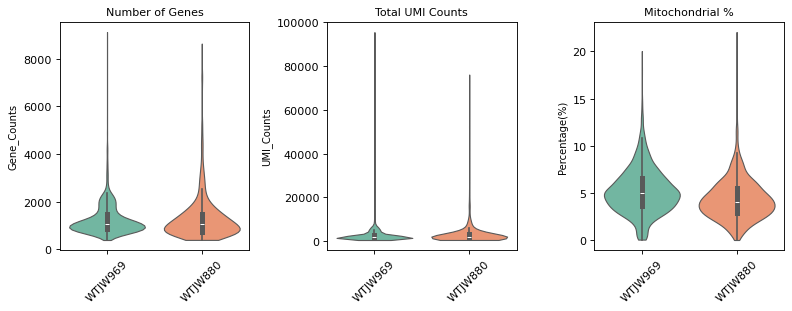
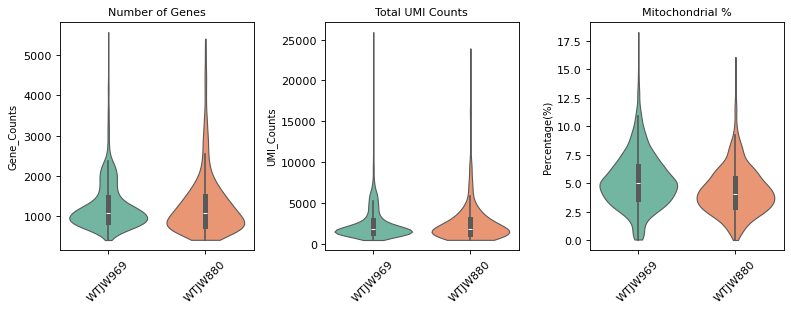
Figure Legend (RNA QC Violin Plot):

The figure below shows the distribution of QC metrics for RNA data before and after filtering, grouped by sample (Sample).

• Pre-QC Violin Plot: QC metric distribution before filtering, including n_genes_by_counts, total_counts, and pct_counts_mt. Used to evaluate raw data quality and identify outliers.
• Post-QC Violin Plot: QC metric distribution after filtering. Low-quality cells (too few/many genes, abnormal UMI counts, high mitochondrial ratio) are removed, improving data quality.
• X-axis: Different samples (Sample), facilitating comparison of QC metrics across samples.
• Y-axis: Values of QC metrics. Violin width indicates cell density in that range; wider means more cells.
• Usage: Evaluate QC filtering effectiveness by comparing distributions before and after, confirming if thresholds are reasonable.

warnings.filterwarnings('ignore')
# --- RNA multi-sample data integration and QC filtering ---

# Read RNA expression data for each sample
obj_rna_list = {}
for i in samples:
    # Build path based on new file hierarchy: ../../data/{top_dir}/methylation/{demo_dir}/{sample}/filtered_feature_bc_matrix
    top_dir = sample_path_config[i]['top_dir']
    demo_dir = sample_path_config[i]['demo_dir']
    s_rna_path = os.path.join('../../',data_root, top_dir, 'methylation', demo_dir, i, 'filtered_feature_bc_matrix')
    obj_rna_list[i] = sc.read_10x_mtx(s_rna_path)

# Merge data from all samples
adata_rna = obj_rna_list[samples[0]].concatenate([obj_rna_list[i] for i in samples[1:]])

# Add sample information
adata_rna.obs['Sample'] = adata_rna.obs['batch'].map(
    {f'{index}': value for index, value in enumerate(samples)}
)

# --- QC filtering ---
# Calculate QC metrics
adata_rna.var['mt'] = adata_rna.var_names.str.startswith('MT-')  # Mitochondrial gene markers
sc.pp.calculate_qc_metrics(adata_rna, qc_vars=['mt'], percent_top=None, log1p=False, inplace=True)

# Save pre-QC statistical information
n_cells_before = adata_rna.n_obs
n_genes_before = adata_rna.n_vars

print(f"质控前细胞数: {n_cells_before}")
print(f"质控前基因数: {n_genes_before}")

# --- Violin plot visualization before QC ---
print("\n=== 质控前质控指标分布 ===")
# sc.pl.violin(adata_rna, keys=['n_genes_by_counts', 'total_counts', 'pct_counts_mt'], 
#              groupby='Sample', rotation=45, multi_panel=True)
fig, (ax1, ax2, ax3) = plt.subplots(1, 3, figsize=(10, 4), dpi=80) 

sc.pl.violin(adata_rna, keys='n_genes_by_counts', groupby='Sample', rotation=45, ax=ax1, show=False, palette=my_palette, stripplot=False, size=1, inner='box', linewidth=1, cut=0)
ax1.set_title("Number of Genes", fontsize=10)
ax1.set_ylabel("Gene_Counts", fontsize=9)
ax1.set_xlabel("")

sc.pl.violin(adata_rna, keys='total_counts', groupby='Sample', rotation=45, ax=ax2, show=False, palette=my_palette, stripplot=False, size=1, inner='box', linewidth=1, cut=0)
ax2.set_title("Total UMI Counts", fontsize=10)
ax2.set_ylabel("UMI_Counts", fontsize=9)
ax2.set_xlabel("")

sc.pl.violin(adata_rna, keys='pct_counts_mt', groupby='Sample', rotation=45, ax=ax3, show=False, palette=my_palette, stripplot=False, size=1, inner='box', linewidth=1, cut=0)
ax3.set_title("Mitochondrial %", fontsize=10)
ax3.set_ylabel("Percentage(%)", fontsize=9)
ax3.set_xlabel("")

plt.tight_layout()
plt.show()

# Filter low-quality cells
# nFeature (n_genes_by_counts): Filter based on number of detected genes per cell (stored in adata_rna.obs['n_genes_by_counts'])
# nCount (total_counts): Filter based on total UMI counts per cell (stored in adata_rna.obs['total_counts'])
# Mitochondrial gene percentage: Filter based on mitochondrial transcript proportion (stored in adata_rna.obs['pct_counts_mt'])

# 1) Filter cells with low gene counts by nFeature
sc.pp.filter_cells(adata_rna, min_genes=200)  # Equivalent to filtering by n_genes_by_counts >= 200

# 2) Filter low-expression genes (genes expressed in fewer than 3 cells)
sc.pp.filter_genes(adata_rna, min_cells=3)

# 3) Further filter by nCount and mitochondrial percentage
adata_rna = adata_rna[(adata_rna.obs['n_genes_by_counts'] >= 200) & (adata_rna.obs['n_genes_by_counts'] <= 10000), :].copy() # nFeature Filtering
adata_rna = adata_rna[(adata_rna.obs['total_counts'] >= 200) & (adata_rna.obs['total_counts'] <= 30000), :].copy()  # nCount Filtering
adata_rna = adata_rna[adata_rna.obs['pct_counts_mt'] < 20, :].copy()  # Mitochondrial gene percentage filtering

print(f"\n质控后细胞数: {adata_rna.n_obs}")
print(f"质控后基因数: {adata_rna.n_vars}")
print(f"过滤掉的细胞数: {n_cells_before - adata_rna.n_obs}")
print(f"过滤掉的基因数: {n_genes_before - adata_rna.n_vars}")

# --- Violin plot visualization after QC ---
print("\n=== 质控后质控指标分布 ===")
fig, (ax1, ax2, ax3) = plt.subplots(1, 3, figsize=(10, 4), dpi=80) 

sc.pl.violin(adata_rna, keys='n_genes_by_counts', groupby='Sample', rotation=45, ax=ax1, show=False, palette=my_palette, stripplot=False, size=1, inner='box', linewidth=1, cut=0)
ax1.set_title("Number of Genes", fontsize=10)
ax1.set_ylabel("Gene_Counts", fontsize=9)
ax1.set_xlabel("")

sc.pl.violin(adata_rna, keys='total_counts', groupby='Sample', rotation=45, ax=ax2, show=False, palette=my_palette, stripplot=False, size=1, inner='box', linewidth=1, cut=0)
ax2.set_title("Total UMI Counts", fontsize=10)
ax2.set_ylabel("UMI_Counts", fontsize=9)
ax2.set_xlabel("")

sc.pl.violin(adata_rna, keys='pct_counts_mt', groupby='Sample', rotation=45, ax=ax3, show=False, palette=my_palette, stripplot=False, size=1, inner='box', linewidth=1, cut=0)
ax3.set_title("Mitochondrial %", fontsize=10)
ax3.set_ylabel("Percentage(%)", fontsize=9)
ax3.set_xlabel("")

plt.tight_layout()
plt.show()

output

质控前细胞数: 2828
质控前基因数: 38606

=== 质控前质控指标分布 ===

质控后细胞数: 2817
质控后基因数: 19405
过滤掉的细胞数: 11
过滤掉的基因数: 19201

=== 质控后质控指标分布 ===

Methylation Data Integration and QC Filtering

This section integrates methylation data from multiple samples, merges QC metadata, and filters based on QC metrics.

Data Integration and Metadata Merging Steps:

1. Data Integration: Read MCDS format methylation data for each sample and merge.
2. Read Metadata: Read cell metadata file and Reads count file for each sample.
3. Methylation Rate Calculation: Calculate CpG and CH methylation rates for each cell.
4. Metadata Merging: Merge calculated QC metrics into adata_met.obs.

QC Filtering Strategy:

• total_cpg_number (Total CpG Sites): Filter cells with total CpG sites < 1000; these cells may have low capture efficiency or poor quality.
• CpG% (CpG Methylation Rate): Filter cells with CpG methylation rate outside 60-100%; these values may be abnormal.
• CH% (CH Methylation Rate): Filter cells with CH methylation rate outside 0-5% (mammalian cell CH% is typically < 5%); abnormally high values may indicate technical issues.

After QC filtering is complete, count cells before and after QC and visualize QC metrics with violin plots.

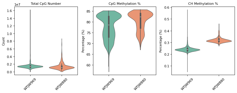
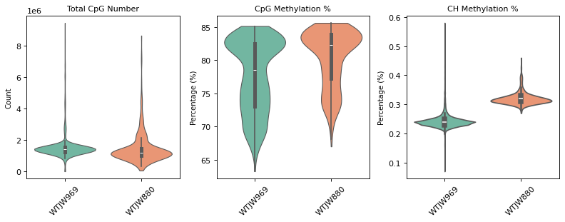
Figure Legend (Methylation QC Violin Plot):

The figure below shows the distribution of QC metrics for methylation data before and after filtering, grouped by sample (Sample).

• Pre-QC Violin Plot: QC metric distribution before filtering, including total_cpg_number, CpG%, and CH%. Used to evaluate raw data quality and identify outliers.
• Post-QC Violin Plot: QC metric distribution after filtering. Low-quality cells (too few CpG sites, abnormal methylation rates) are removed, improving data quality.
• X-axis: Different samples (Sample), facilitating comparison of QC metrics across samples.
• Y-axis: Values of QC metrics. Violin width indicates cell density in that range; wider means more cells.
• Usage: Evaluate QC filtering effectiveness by comparing distributions before and after, confirming if thresholds are reasonable.

warnings.filterwarnings('ignore')
# --- Methylation data multi-sample integration ---

# Read MCDS format methylation data for each sample
obj_met_list = {}
mcds_paths = {}
for i in samples:
    # Build path based on new file hierarchy: data/{top_dir}/methylation/{demo_dir}/{sample}/allcools_generate_datasets/{sample}.mcds
    top_dir = sample_path_config[i]['top_dir']
    demo_dir = sample_path_config[i]['demo_dir']
    mcds_path = os.path.join('../../',data_root, top_dir, 'methylation', demo_dir, i, 'allcools_generate_datasets', f'{i}.mcds')
    
    mcds_paths[i] = mcds_path
    mcds = MCDS.open(mcds_path, obs_dim='cell', var_dim=var_dim)
    adata = mcds.get_score_adata(mc_type=mc_type, quant_type=quant_type, sparse=True)
    obj_met_list[i] = adata

# Merge data from all samples
adata_met = obj_met_list[samples[0]].concatenate([obj_met_list[i] for i in samples[1:]])

# Save raw data
adata_met.layers['raw'] = adata_met.X.copy()

# Add sample information
adata_met.obs['Sample'] = adata_met.obs['batch'].map(
    {f'{index}': value for index, value in enumerate(samples)}
)

# --- Helper function to calculate CpG and CH methylation rates ---
def compute_cg_ch_level(df):
    # Calculate CpG and CH methylation levels
    cg_cov_col = [i for i in df.columns[df.columns.str.startswith('CG')].to_list() if i.endswith('_cov')]
    cg_mc_col = [i for i in df.columns[df.columns.str.startswith('CG')].to_list() if i.endswith('_mc')]
    ch_cov_col = [i for i in df.columns[df.columns.str.contains('^(CT|CC|CA)')].to_list() if i.endswith('_cov')]
    ch_mc_col = [i for i in df.columns[df.columns.str.contains('^(CT|CC|CA)')].to_list() if i.endswith('_mc')]
    
    df['CpG_cov'] = df[cg_cov_col].sum(axis=1)
    df['CpG_mc'] = df[cg_mc_col].sum(axis=1)
    df['CpG%'] = round(df['CpG_mc'] * 100 / df['CpG_cov'], 2)
    
    df['CH_cov'] = df[ch_cov_col].sum(axis=1)
    df['CH_mc'] = df[ch_mc_col].sum(axis=1)
    df['CH%'] = round(df['CH_mc'] * 100 / df['CH_cov'], 2)

    return df

# --- Read and merge QC metadata ---
suffix_map = {f'{value}': index for index, value in enumerate(samples)}
meta_list = list()
keep_col = ['barcode', 'total_cpg_number', 'genome_cov', 'reads_counts', 'CpG%', 'CH%']

for i in samples:
    # Build paths based on the new file hierarchy structure
    top_dir = sample_path_config[i]['top_dir']
    demo_dir = sample_path_config[i]['demo_dir']
    
    # Read cell metadata file: ../../data/{top_dir}/methylation/{demo_dir}/{sample}/split_bams/{sample}_cells.csv
    s_cells_meta_path = os.path.join('../../',data_root, top_dir, 'methylation', demo_dir, i, 'split_bams', f'{i}_cells.csv')
    s_cells_meta = pd.read_csv(s_cells_meta_path, header=0)
    s_cells_meta['barcode'] = [b.replace('_allc.gz', '') for b in s_cells_meta['cell_barcode']]
    
    # Read Reads count file: ../../data/{top_dir}/methylation/{demo_dir}/{sample}/split_bams/filtered_barcode_reads_counts.csv
    s_reads_counts_path = os.path.join('../../',data_root, top_dir, 'methylation', demo_dir, i, 'split_bams', 'filtered_barcode_reads_counts.csv')
    s_reads_counts = pd.read_csv(s_reads_counts_path, header=0)
    
    # Merge data and calculate methylation rate
    s_merged_df = s_cells_meta.merge(s_reads_counts, how='inner', left_on='barcode', right_on='barcode')
    s_merged_df = compute_cg_ch_level(s_merged_df)
    s_merged_df = s_merged_df[keep_col]
    
    # If multi-sample, add sample identifier to barcode
    if len(samples) > 1:
        s_merged_df['barcode'] = [f'{b}-{suffix_map[i]}' for b in s_merged_df['barcode']]
    
    meta_list.append(s_merged_df)

# Merge metadata from all samples to adata_met.obs
adata_met.obs = adata_met.obs.merge(
    pd.concat(meta_list).set_index('barcode'), 
    how='left', 
    left_index=True, 
    right_index=True
)

# --- Methylation data QC filtering ---
# Save pre-QC statistical information
n_cells_before = adata_met.n_obs

print(f"质控前细胞数: {n_cells_before}")

# --- Violin plot visualization before QC ---
print("\n=== 质控前质控指标分布 ===")
fig, (ax1, ax2, ax3) = plt.subplots(1, 3, figsize=(10, 4), dpi=80)

# 1. Total CpG Number
sc.pl.violin(adata_met, keys='total_cpg_number', groupby='Sample', rotation=45, ax=ax1, show=False, palette=my_palette, stripplot=False, size=1, inner='box', linewidth=1, cut=0)
ax1.set_title("Total CpG Number", fontsize=10)
ax1.set_ylabel("Count", fontsize=9)
ax1.set_xlabel("")

# 2. CpG%
sc.pl.violin(adata_met, keys='CpG%', groupby='Sample', rotation=45, ax=ax2, show=False, palette=my_palette, stripplot=False, size=1, inner='box', linewidth=1, cut=0)
ax2.set_title("CpG Methylation %", fontsize=10)
ax2.set_ylabel("Percentage (%)", fontsize=9)
ax2.set_xlabel("")

# 3. CH%
sc.pl.violin(adata_met, keys='CH%', groupby='Sample', rotation=45, ax=ax3, show=False, palette=my_palette, stripplot=False, size=1, inner='box', linewidth=1, cut=0)
ax3.set_title("CH Methylation %", fontsize=10)
ax3.set_ylabel("Percentage (%)", fontsize=9)
ax3.set_xlabel("")

plt.tight_layout()
plt.show()


# Filter low-quality cells based on QC metrics
# total_cpg_number: Filter cells with too few total CpG sites (threshold can be adjusted based on actual situation)
# CpG%: Filter cells with abnormal CpG methylation rates (typically mammalian cells have CpG% between 40-80%)
# CH%: Filter cells with abnormal CH methylation rates (typically mammalian cells have low CH%, < 5%)

# Check for missing values and handle them
if 'total_cpg_number' in adata_met.obs.columns:
    adata_met = adata_met[adata_met.obs['total_cpg_number'].notna(), :].copy()
    adata_met = adata_met[(adata_met.obs['total_cpg_number'] >= 100) & (adata_met.obs['total_cpg_number'] <= 10000000), :].copy()

if 'CpG%' in adata_met.obs.columns:
    adata_met = adata_met[adata_met.obs['CpG%'].notna(), :].copy()
    adata_met = adata_met[(adata_met.obs['CpG%'] >= 60) & (adata_met.obs['CpG%'] <= 100), :].copy()

if 'CH%' in adata_met.obs.columns:
    adata_met = adata_met[adata_met.obs['CH%'].notna(), :].copy()
    adata_met = adata_met[(adata_met.obs['CH%'] >= 0) & (adata_met.obs['CH%'] <= 5), :].copy()

print(f"质控后细胞数: {adata_met.n_obs}")
print(f"过滤掉的细胞数: {n_cells_before - adata_met.n_obs}")

# --- Violin plot visualization after QC ---
print("\n=== 质控后质控指标分布 ===")
fig, (ax1, ax2, ax3) = plt.subplots(1, 3, figsize=(10, 4), dpi=80)

# 1. Total CpG Number
sc.pl.violin(adata_met, keys='total_cpg_number', groupby='Sample', rotation=45, ax=ax1, show=False, palette=my_palette, stripplot=False, size=1, inner='box', linewidth=1, cut=0)
ax1.set_title("Total CpG Number", fontsize=10)
ax1.set_ylabel("Count", fontsize=9)
ax1.set_xlabel("")

# 2. CpG%
sc.pl.violin(adata_met, keys='CpG%', groupby='Sample', rotation=45, ax=ax2, show=False, palette=my_palette, stripplot=False, size=1, inner='box', linewidth=1, cut=0)
ax2.set_title("CpG Methylation %", fontsize=10)
ax2.set_ylabel("Percentage (%)", fontsize=9)
ax2.set_xlabel("")

# 3. CH%
sc.pl.violin(adata_met, keys='CH%', groupby='Sample', rotation=45, ax=ax3, show=False, palette=my_palette, stripplot=False, size=1, inner='box', linewidth=1.5, cut=0)
ax3.set_title("CH Methylation %", fontsize=10)
ax3.set_ylabel("Percentage (%)", fontsize=9)
ax3.set_xlabel("")

plt.tight_layout()
plt.show()

output

Loading chunk 0-2196/2196
Loading chunk 0-442/442
质控前细胞数: 2638

=== 质控前质控指标分布 ===

质控后细胞数: 2631
过滤掉的细胞数: 7

=== 质控后质控指标分布 ===

RNA and Methylation Data Barcode Association, Intersection, and Doublet Filtering

This section first associates RNA and methylation Barcodes based on kit type, then identifies common cells (barcode intersection) in both datasets, and finally removes doublet cells based on the doublet table.

Steps:

1. Barcode Association: Associate Barcodes of RNA and methylation data according to kit type (DD-MET3/DD-MET5).
2. Barcode Intersection: Calculate barcode intersection of RNA and methylation data to ensure cell consistency between the two datasets.
3. Doublet Filtering: Read doublet tables for each sample and remove doublet cells from RNA and methylation data.

Associate RNA and methylation Barcodes based on kit type to establish cell correspondence between the two datasets.

• DD-MET3: RNA and methylation data use different Barcodes and need to be associated via a mapping file. Please download the Barcode mapping file DD-M_bUCB3_whitelist.csv locally first. Then read the Barcode mapping file (DD-M_bUCB3_whitelist.csv) to establish correspondence between RNA Barcodes (gex_cb) and Methylation Barcodes (m_cb), and create rna_meta mapping table for subsequent use.
• DD-MET5: RNA and methylation data use the same Barcode, no mapping is needed; skip this step directly.

TIP

The mapping relationship established in this step (rna_meta) will be used for subsequent doublet filtering and cell type annotation transfer.

# --- RNA and Methylation Data Association (Supports sample-specific config: some DD-MET3 need mapping, some DD-MET5 do not) ---

print("=== 数据状态检查 ===")
print(f"RNA 数据细胞数: {len(adata_rna.obs)}")
print(f"甲基化数据细胞数: {len(adata_met.obs)}")
if len(adata_rna.obs) == 0:
    raise ValueError("RNA 数据为空，无法建立映射关系。请检查前面的数据加载和质控步骤。")
if len(adata_met.obs) == 0:
    raise ValueError("甲基化数据为空，无法建立映射关系。请检查前面的质控过滤步骤。")

suffix_map = {s: i for i, s in enumerate(samples)}  # sample -> batch index

# If DD-MET3 samples exist, load barcode mapping file (load only once)
if any(reagent_type_map.get(s, reagent_type) == "DD-MET3" for s in samples):
    mapping_file = "DD-M_bUCB3_whitelist.csv"
    if not os.path.exists(mapping_file):
        raise FileNotFoundError("未找到映射文件：DD-M_bUCB3_whitelist.csv，请确认文件路径。")
    gex_mc_bc_map = pd.read_csv(mapping_file, index_col=None)
    if 'gex_cb' not in gex_mc_bc_map.columns or 'm_cb' not in gex_mc_bc_map.columns:
        raise ValueError(f"映射文件格式错误：应包含 'gex_cb' 和 'm_cb' 列，实际列名: {list(gex_mc_bc_map.columns)}")
    print(f"映射文件路径: {mapping_file}，记录数: {len(gex_mc_bc_map)}")
else:
    gex_mc_bc_map = None

rna_meta_list = []
for sample in samples:
    rt = reagent_type_map.get(sample, reagent_type)
    rna_obs_s = adata_rna.obs[adata_rna.obs['Sample'] == sample]
    met_barcodes_s = set(adata_met.obs.index[adata_met.obs['Sample'] == sample])
    suf = suffix_map[sample]

    if rt == "DD-MET3":
        # This sample requires barcode mapping
        rm = rna_obs_s.copy()
        rm["rna_bc_with_suffix"] = rm.index
        rm["gex_cb"] = [re.sub(r'-.*$', '', b) for b in rm["rna_bc_with_suffix"]]
        rm = rm.merge(gex_mc_bc_map, how='left', left_on='gex_cb', right_on='gex_cb')
        rm = rm.dropna(subset=['m_cb'])
        rm["m_cb"] = rm["m_cb"].astype(str) + "-" + str(suf)
        rm = rm[rm["m_cb"].isin(met_barcodes_s)]
        rm.index = rm["m_cb"]
        rna_meta_list.append(rm)
        print(f"  {sample} (DD-MET3): 映射后保留 {len(rm)} 个共同细胞")
    else:
        # DD-MET5: Same barcode, keep only cells present in both RNA and methylation
        common_s = set(rna_obs_s.index) & met_barcodes_s
        rm = pd.DataFrame({"rna_bc_with_suffix": list(common_s), "m_cb": list(common_s), "gex_cb": [re.sub(r'-.*$', '', b) for b in common_s]})
        rm.index = rm["m_cb"]
        rna_meta_list.append(rm)
        print(f"  {sample} (DD-MET5): 不映射，共有 {len(rm)} 个共同细胞")

if rna_meta_list:
    rna_meta = pd.concat(rna_meta_list, axis=0)
    rna_met_mapping = rna_meta[["gex_cb", "m_cb", "rna_bc_with_suffix"]].copy()
    print(f"\n=== 汇总 ===")
    print(f"成功建立关联的细胞数: {len(rna_meta)}")
else:
    rna_meta = None
    rna_met_mapping = None

output

=== 数据状态检查 ===
RNA 数据细胞数: 2817
甲基化数据细胞数: 2631
映射文件路径: DD-M_bUCB3_whitelist.csv，记录数: 248832
WTJW969 (DD-MET5): 不映射，共有 2187 个共同细胞
WTJW880 (DD-MET3): 映射后保留 438 个共同细胞

=== 汇总 ===
成功建立关联的细胞数: 2625

# --- Intersect and filter RNA and methylation data barcodes ---
# Since RNA and methylation data were QC filtered separately, need to ensure cells in both datasets are consistent
# If mapping table rna_meta exists (contains DD-MET3 or mixed samples), intersect by mapping; otherwise intersect directly by barcode (all DD-MET5)

print("=== RNA 和甲基化数据 barcode 取交集 ===")

if rna_meta is not None and len(rna_meta) > 0:
    # DD-MET3: Intersect via mapping relationship
    # rna_meta index is methylation barcode (m_cb), contains corresponding RNA barcode information
    # Use existing mapping in rna_meta to intersect
    
    if rna_meta is None or len(rna_meta) == 0:
        raise ValueError("rna_meta 为空，请先执行 barcode 关联步骤（Cell 15）")
    
    # Get valid methylation barcodes in mapping table (those with established mapping relationships)
    mapped_met_barcodes = set(rna_meta.index)
    
    # Get barcodes actually present in methylation data
    met_barcodes = set(adata_met.obs.index)
    
    # Get barcodes actually present in RNA data
    rna_barcodes_with_suffix = set(adata_rna.obs.index)
    
    print(f"RNA 数据细胞数: {len(rna_barcodes_with_suffix)}")
    print(f"甲基化数据细胞数: {len(met_barcodes)}")
    print(f"映射表中有效的甲基化 barcode 数: {len(mapped_met_barcodes)}")
    
    # Intersect: Barcodes present in mapping table and also in methylation data
    common_met_barcodes = mapped_met_barcodes & met_barcodes
    print(f"映射表与甲基化数据的交集（甲基化 barcode）: {len(common_met_barcodes)}")
    
    if len(common_met_barcodes) == 0:
        print("⚠️  警告：映射表与甲基化数据没有交集！")
        print("可能的原因：")
        print("1. 映射关系建立失败")
        print("2. 甲基化数据在质控步骤中被过度过滤")
        print("3. barcode 格式不匹配")
        raise ValueError("无法找到交集，请检查映射关系和数据状态。")
    
    # Find corresponding RNA barcode (with suffix) via mapping relationship
    rna_meta_filtered = rna_meta.loc[list(common_met_barcodes), :]
    common_rna_barcodes_with_suffix = set(rna_meta_filtered["rna_bc_with_suffix"].values)
    
    print(f"通过映射关系找到的 RNA barcode 数: {len(common_rna_barcodes_with_suffix)}")
    
    # Ensure RNA barcode exists in RNA data
    common_rna_barcodes_with_suffix = common_rna_barcodes_with_suffix & rna_barcodes_with_suffix
    print(f"RNA barcode 与 RNA 数据的交集: {len(common_rna_barcodes_with_suffix)}")
    
    if len(common_rna_barcodes_with_suffix) == 0:
        print("⚠️  警告：映射后的 RNA barcode 在 RNA 数据中不存在！")
        raise ValueError("无法找到有效的 RNA barcode，请检查映射关系和 RNA 数据。")
    
    # Update corresponding methylation barcode (keep only those existing in RNA barcode)
    rna_meta_filtered = rna_meta_filtered[rna_meta_filtered["rna_bc_with_suffix"].isin(common_rna_barcodes_with_suffix)]
    common_met_barcodes = set(rna_meta_filtered.index)
    
    print(f"\n最终交集统计：")
    print(f"  交集细胞数（甲基化 barcode）: {len(common_met_barcodes)}")
    print(f"  交集细胞数（RNA barcode）: {len(common_rna_barcodes_with_suffix)}")
    
    # Filter both datasets, keeping only cells in the intersection
    print(f"\n开始过滤数据...")
    adata_rna_before = adata_rna.n_obs
    adata_met_before = adata_met.n_obs
    
    adata_rna = adata_rna[adata_rna.obs.index.isin(common_rna_barcodes_with_suffix), :].copy()
    adata_met = adata_met[adata_met.obs.index.isin(common_met_barcodes), :].copy()
    
    # Update rna_meta, keeping only filtered mapping relationships
    rna_meta = rna_meta.loc[list(common_met_barcodes), :]
    
    print(f"\n过滤结果：")
    print(f"  RNA 数据: {adata_rna_before} → {adata_rna.n_obs} (删除 {adata_rna_before - adata_rna.n_obs} 个)")
    print(f"  甲基化数据: {adata_met_before} → {adata_met.n_obs} (删除 {adata_met_before - adata_met.n_obs} 个)")
    
    # Verify consistency after filtering
    if adata_rna.n_obs != adata_met.n_obs:
        print(f"⚠️  警告：过滤后 RNA 和甲基化数据的细胞数不一致！")
        print(f"  RNA: {adata_rna.n_obs}, 甲基化: {adata_met.n_obs}")
    else:
        print(f"✅ 过滤后两个数据集的细胞数一致: {adata_rna.n_obs}")
    
else:
    # No mapping table or empty: RNA and methylation use same Barcode, take intersection directly (also enters this branch if all DD-MET5 and no cells)
    rna_barcodes = set(adata_rna.obs.index)
    met_barcodes = set(adata_met.obs.index)
    
    # Calculate intersection
    common_barcodes = rna_barcodes & met_barcodes
    
    print(f"RNA 数据细胞数: {len(rna_barcodes)}")
    print(f"甲基化数据细胞数: {len(met_barcodes)}")
    print(f"交集细胞数: {len(common_barcodes)}")
    print(f"仅在 RNA 数据中的细胞数: {len(rna_barcodes - met_barcodes)}")
    print(f"仅在甲基化数据中的细胞数: {len(met_barcodes - rna_barcodes)}")
    
    if len(common_barcodes) == 0:
        print("⚠️  警告：RNA 和甲基化数据没有交集！")
        print("可能的原因：")
        print("1. 两个数据集的 barcode 格式不一致")
        print("2. 质控过滤后没有共同细胞")
        raise ValueError("无法找到交集，请检查数据状态和 barcode 格式。")
    
    # Filter both datasets, keeping only cells in the intersection
    print(f"\n开始过滤数据...")
    adata_rna_before = adata_rna.n_obs
    adata_met_before = adata_met.n_obs
    
    adata_rna = adata_rna[adata_rna.obs.index.isin(common_barcodes), :].copy()
    adata_met = adata_met[adata_met.obs.index.isin(common_barcodes), :].copy()
    
    print(f"\n过滤结果：")
    print(f"  RNA 数据: {adata_rna_before} → {adata_rna.n_obs} (删除 {adata_rna_before - adata_rna.n_obs} 个)")
    print(f"  甲基化数据: {adata_met_before} → {adata_met.n_obs} (删除 {adata_met_before - adata_met.n_obs} 个)")
    
    # Verify consistency after filtering
    if adata_rna.n_obs != adata_met.n_obs:
        print(f"⚠️  警告：过滤后 RNA 和甲基化数据的细胞数不一致！")
        print(f"  RNA: {adata_rna.n_obs}, 甲基化: {adata_met.n_obs}")
    else:
        print(f"✅ 过滤后两个数据集的细胞数一致: {adata_rna.n_obs}")

output

=== RNA 和甲基化数据 barcode 取交集 ===
RNA 数据细胞数: 2817
甲基化数据细胞数: 2631
映射表中有效的甲基化 barcode 数: 2625
映射表与甲基化数据的交集（甲基化 barcode）: 2625
通过映射关系找到的 RNA barcode 数: 2625
RNA barcode 与 RNA 数据的交集: 2625

最终交集统计：
交集细胞数（甲基化 barcode）: 2625
交集细胞数（RNA barcode）: 2625

开始过滤数据...n
过滤结果：
RNA 数据: 2817 → 2625 (删除 192 个)
甲基化数据: 2631 → 2625 (删除 6 个)
✅ 过滤后两个数据集的细胞数一致: 2625

Remove Doublets Based on Doublet Table

This section removes doublets from RNA and methylation data based on doublet identification results for each sample.

Data Source: The {sample}_doublet.txt file comes from the analysis results of Methylation+RNA Dual-omics - Doublet Detection.ipynb, containing identified doublet information for each sample.

Processing Logic:

• Read the doublet table for each sample ({sample}_doublet.txt) to get doublet barcodes for methylation data (m_cb column).
• Process differently according to kit type: * DD-MET3: Convert methylation barcode to RNA barcode via mapping file, then remove from both datasets respectively. * DD-MET5: Methylation barcode is RNA barcode, directly use the same barcode to remove from both datasets.
• Output cell count statistics before and after deletion.

TIP

If doublet removal is not required, this cell can be skipped.

# --- Remove doublets based on doublet table ---
doublet_df_column_name = "met_is_doublet"
# Read doublet tables for each sample and merge
doublet_met_barcodes = set()  # Doublet barcodes for methylation data (used to remove from methylation data)
doublet_rna_barcodes = set()  # RNA data doublet barcode (used to remove RNA data)
suffix_map = {f'{value}': index for index, value in enumerate(samples)}

for sample in samples:
    doublet_path = f"{sample}_doublet.txt"
    if os.path.exists(doublet_path):
        doublet_df = pd.read_csv(doublet_path, sep='\t')
        # Determine how to identify doublets based on doublet_df column names
        if doublet_df_column_name == 'met_is_doublet':
            # If column name is "met_is_doublet", use met_is_doublet == True to identify doublets
            sample_doublets_met = doublet_df[doublet_df['met_is_doublet'] == True]['m_cb'].tolist()
        elif doublet_df_column_name == 'cell_multi_highlight':
            # If column name is "cell_multi_highlight", then 'multi_cells' under this column are doublets
            sample_doublets_met = doublet_df[doublet_df['cell_multi_highlight'] == 'multi_cells']['m_cb'].tolist()
        elif doublet_df_column_name == 'cell_multi_highlight':
            sample_doublets_met = doublet_df[doublet_df['rna_doublet'] == 'doublet']['m_cb'].tolist()
        else:
            raise ValueError(f"doublet 文件 {doublet_path} 中未找到预期的列名。期望列名：'met_is_doublet' 或 'cell_multi_highlight'，实际列名：{list(doublet_df.columns)}")
        
        # Add sample suffix to methylation barcode (used for removal from methylation data)
        if len(samples) > 1:
            sample_doublets_met_with_suffix = [f"{b}-{suffix_map[sample]}" for b in sample_doublets_met]
        else:
            sample_doublets_met_with_suffix = sample_doublets_met
        doublet_met_barcodes.update(sample_doublets_met_with_suffix)
        rt = reagent_type_map.get(sample, reagent_type)
        
        # Perform different processing based on kit type
        if rt == "DD-MET3":
            # DD-MET3: Need to convert methylation barcode to RNA barcode
            # Convert methylation barcode to RNA barcode via mapping file
            sample_gex_mc_map = gex_mc_bc_map[gex_mc_bc_map['m_cb'].isin(sample_doublets_met)]
            sample_doublets_rna = sample_gex_mc_map['gex_cb'].tolist()
            # Add sample suffix to RNA barcode
            if len(samples) > 1:
                sample_doublets_rna_with_suffix = [f"{b}-{suffix_map[sample]}" for b in sample_doublets_rna]
            else:
                sample_doublets_rna_with_suffix = sample_doublets_rna
            doublet_rna_barcodes.update(sample_doublets_rna_with_suffix)
        elif rt == "DD-MET5":
            # DD-MET5: Methylation barcode is RNA barcode, use directly
            doublet_rna_barcodes.update(sample_doublets_met_with_suffix)
        else:
            raise ValueError(f"不支持的试剂盒类型: {reagent_type}，请设置为 'DD-MET3' 或 'DD-MET5'")
        
        print(f"{sample}: 检测到 {len(sample_doublets_met)} 个 doublet 细胞")
    else:
        print(f"警告：未找到 {sample} 的 doublet 文件 {doublet_path}")

if doublet_met_barcodes:
    print(f"\n总共检测到的 doublet 细胞数: {len(doublet_met_barcodes)}")
    print(f"试剂盒类型: {reagent_type}")
    
    # Remove doublets from methylation data (using methylation barcode)
    adata_met = adata_met[~adata_met.obs.index.isin(doublet_met_barcodes), :].copy()
    
    # Remove doublets from RNA data (using RNA barcode)
    adata_rna = adata_rna[~adata_rna.obs.index.isin(doublet_rna_barcodes), :].copy()
    
    print(f"删除 doublet 后 RNA 数据细胞数: {adata_rna.n_obs}")
    print(f"删除 doublet 后甲基化数据细胞数: {adata_met.n_obs}")
else:
    print("警告：未找到任何 doublet 文件，跳过 doublet 过滤")

output

WTJW969: 检测到 272 个 doublet 细胞
WTJW880: 检测到 134 个 doublet 细胞

总共检测到的 doublet 细胞数: 406
试剂盒类型: DD-MET3
删除 doublet 后 RNA 数据细胞数: 2226
删除 doublet 后甲基化数据细胞数: 2226

Single-cell RNA Sequencing Data Multi-sample Integration Analysis Pipeline

This section performs normalization, feature selection, dimensionality reduction, batch correction, and clustering analysis on QC-filtered RNA data.

Data Normalization and Dimensionality Reduction Analysis

warnings.filterwarnings('ignore')
# --- RNA data normalization and dimensionality reduction analysis ---

# Normalization: Total count normalization to eliminate sequencing depth differences between cells
sc.pp.normalize_total(adata_rna, inplace=True)

# Log Transformation: log(x + 1)
sc.pp.log1p(adata_rna)

# Identify highly variable genes (2000), which best reflect biological differences between cells
sc.pp.highly_variable_genes(adata_rna, n_bins=100, n_top_genes=2000)

# Save raw data, then keep only highly variable genes
adata_rna.raw = adata_rna
adata_rna = adata_rna[:, adata_rna.var.highly_variable]

# Z-score normalization of highly variable genes
sc.pp.scale(adata_rna, max_value=10)

# Principal Component Analysis (PCA)
sc.tl.pca(adata_rna)

# Harmony Batch Effect Correction
ho = run_harmony(
    adata_rna.obsm['X_pca'],
    meta_data=adata_rna.obs,
    vars_use='Sample',
    random_state=0,
    max_iter_harmony=20
)
adata_rna.obsm['X_pca_harmony'] = ho.Z_corr.T

# Use Harmony corrected results for subsequent analysis
reduc_use = 'X_pca_harmony'

# Build KNN Graph
sc.pp.neighbors(adata_rna, n_neighbors=30, use_rep=reduc_use)

# UMAP Dimensionality Reduction Visualization
sc.tl.umap(adata_rna)

# t-SNE Dimensionality Reduction Visualization
sc.tl.tsne(adata_rna, use_rep=reduc_use)

# Leiden Clustering
sc.tl.leiden(adata_rna, resolution=1)

output

2026-01-28 16:12:37,786 - harmonypy - INFO - Computing initial centroids with sklearn.KMeans...n 2026-01-28 16:12:38,283 - harmonypy - INFO - sklearn.KMeans initialization complete.
2026-01-28 16:12:38,318 - harmonypy - INFO - Iteration 1 of 20
2026-01-28 16:12:40,373 - harmonypy - INFO - Iteration 2 of 20
2026-01-28 16:12:42,297 - harmonypy - INFO - Converged after 2 iterations

RNA Single-omics Cell Annotation

Figure Legend (RNA UMAP - Leiden Clustering):

The figure below shows the cell distribution of RNA data in UMAP space, colored by Leiden clustering results.

• X and Y axes: Two main dimensions after UMAP dimensionality reduction (UMAP1 and UMAP2), used to display cell similarity relationships in high-dimensional data in 2D space.
• Color: Colors represent Leiden clustering results; each cluster may correspond to one or more cell types.
• Points: Each point represents a cell; position reflects similarity to other cells. Similar cells cluster together in UMAP space.
• Usage: Evaluate clustering performance, identify cell subpopulations, and discover potential cell types.

warnings.filterwarnings('ignore')
sc.set_figure_params(scanpy=True, fontsize=12, facecolor='white', figsize=(6, 6))
sc.pl.umap(adata_rna, color='leiden', s=35, palette=my_palette, frameon=True)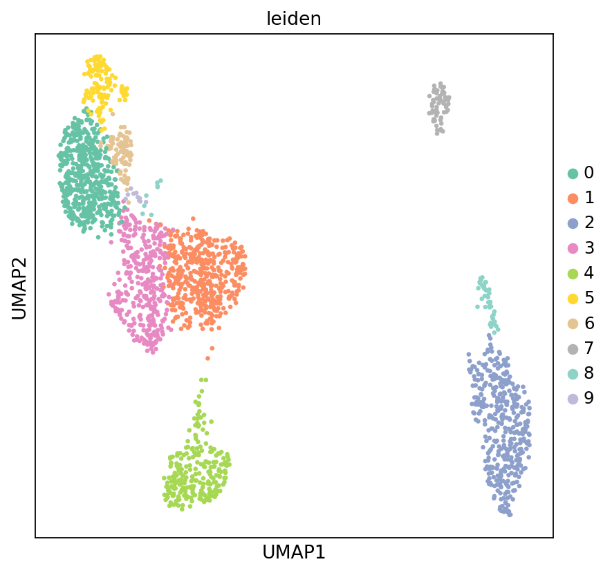

Figure Legend (RNA UMAP - Marker Gene Expression):

The figure below shows the expression distribution of marker genes in RNA data within UMAP space.

• X and Y axes: Two main dimensions after UMAP dimensionality reduction (UMAP1 and UMAP2).
• Color: Intensity represents marker gene expression level; darker means higher expression. Markers include: CD3D (T cells), NKG7 (NK cells), CD8A (CD8+ T), CD4 (CD4+ T), CD79A/MS4A1 (B cells), JCHAIN (Plasma cells), LYZ (Monocytes), LILRA4 (pDC).
• Points: Each point represents a cell.
• Usage: Preliminarily identify and verify different cell types via marker gene expression patterns, assisting cell type annotation.

colors = ["#F5E6CC", "#FDBB84", "#E34A33", "#7F0000"]
my_warm_cmap = mcolors.LinearSegmentedColormap.from_list("white_orange_red", colors, N=256)

marker_names = ["CD3D","NKG7","CD8A","CD4","CCR7","CD79A","MS4A1","LYZ","FCN1","FCGR3A","CST3"]
sc.pl.umap(
    adata_rna, 
    color=marker_names, 
    ncols=4,            
    color_map=my_warm_cmap, 
    vmax='p99',         
    s=10,               
    frameon=False,      
    vmin=0,
    show=False 
)

plt.gcf().set_size_inches(16, 8) 
plt.show()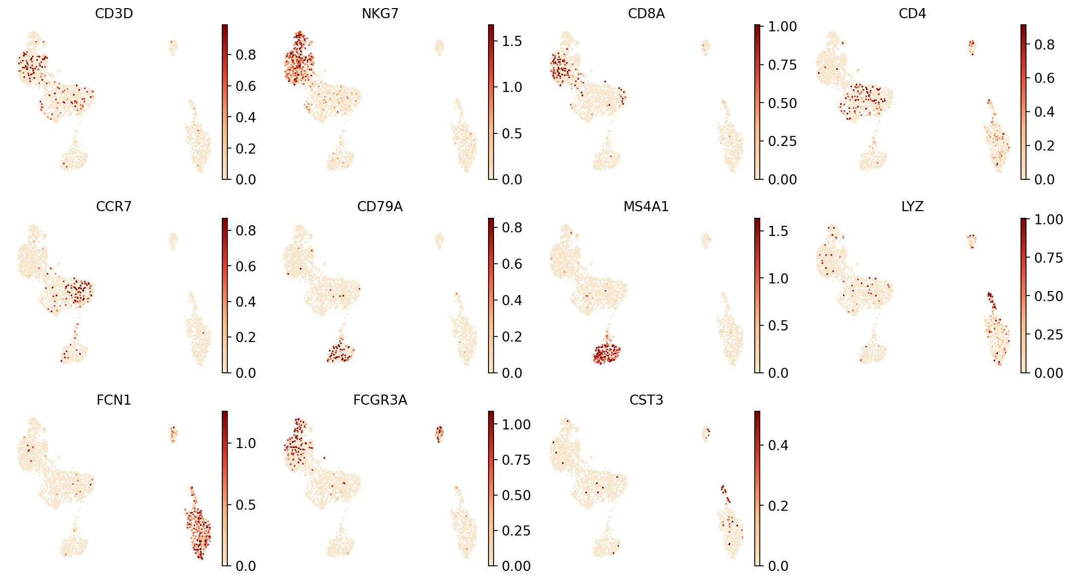

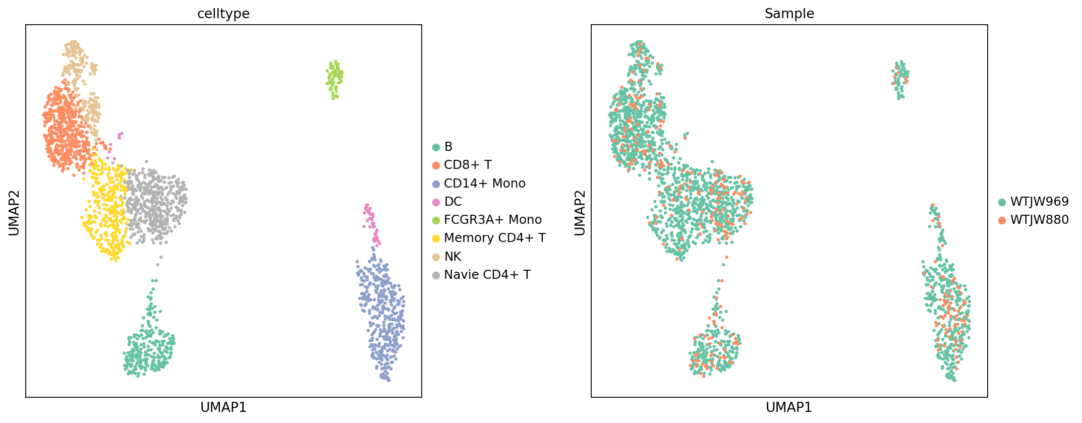
Figure Legend (RNA UMAP - Cell Type and Sample):

The figure below shows the distribution of RNA data in UMAP space, colored by cell type (celltype) and sample (Sample).

• X and Y axes: Two main dimensions after UMAP dimensionality reduction (UMAP1 and UMAP2).
• Color (celltype Plot): Colors represent cell types, showing overall distribution after annotation.
• Color (Sample Plot): Colors represent samples, used to evaluate batch effects and cell type composition differences.
• Points: Each point represents a cell.
• Usage: Evaluate cell type annotation performance, check for batch effects between samples, and compare cell type composition across samples.

celltype = {
    '0': 'CD8+ T',
    '1': 'Navie CD4+ T',
    '2': 'CD14+ Mono',
    '3': 'Memory CD4+ T',
    '4': 'B',
    '5': 'NK',
    '6': 'NK',
    '7': 'FCGR3A+ Mono',
    '8': 'DC',
    '9': 'CD8+ T'
}

adata_rna.obs['celltype'] = adata_rna.obs['leiden'].map(celltype)

sc.set_figure_params(scanpy=True, fontsize=12, facecolor='white', figsize=(6, 6))
sc.pl.umap(
    adata_rna, 
    color=['celltype', 'Sample'], 
    ncols=2,
    s=35,
    wspace=0.3,
    palette=my_palette
)

adata_rna.write("adata_rna.h5ad")

Single-cell Methylation Sequencing Data Multi-sample Integration Analysis Pipeline

This section performs preprocessing, dimensionality reduction, batch correction, clustering analysis, and cell type annotation transfer on QC-filtered methylation data.

Data Preprocessing and Dimensionality Reduction Analysis

This section performs preprocessing, dimensionality reduction clustering, and batch correction on QC-filtered methylation data.

# --- Methylation data preprocessing and dimensionality reduction analysis ---

# Matrix Binarization: Set 95% threshold for data binarization to highlight significant epigenetic differences
binarize_matrix(adata_met, cutoff=0.95)

# Region Filtering: Smartly filter genomic regions
filter_regions(adata_met)

# LSI Dimensionality Reduction: Uses ARPACK algorithm for linear dimensionality reduction to extract principal components of genomic methylation patterns
lsi(adata_met, algorithm='arpack', obsm='X_lsi')

# Significant Principal Component Test: Keep only significant components with p < 0.1
significant_pc_test(adata_met, p_cutoff=0.1, obsm='X_lsi', update=True)

# Harmony Batch Effect Correction
ho = run_harmony(
    adata_met.obsm['X_lsi'],
    meta_data=adata_met.obs,
    vars_use='Sample',
    random_state=0,
    max_iter_harmony=20
)
adata_met.obsm['X_lsi_harmony'] = ho.Z_corr.T

# Use Harmony corrected results for subsequent analysis
reduc_use = 'X_lsi_harmony'

# Build KNN Graph
sc.pp.neighbors(adata_met, n_neighbors=30, use_rep=reduc_use)

# UMAP Dimensionality Reduction Visualization
sc.tl.umap(adata_met)

# t-SNE Dimensionality Reduction Visualization
sc.tl.tsne(adata_met, use_rep=reduc_use)

# Leiden Clustering
sc.tl.leiden(adata_met, resolution=0.5)

output

125666 regions remained.


2026-01-28 16:13:44,567 - harmonypy - INFO - Computing initial centroids with sklearn.KMeans...n

13 components passed P cutoff of 0.1.
Changing adata.obsm['X_pca'] from shape (2226, 100) to (2226, 13)


2026-01-28 16:13:44,833 - harmonypy - INFO - sklearn.KMeans initialization complete.
2026-01-28 16:13:44,950 - harmonypy - INFO - Iteration 1 of 20
2026-01-28 16:13:49,462 - harmonypy - INFO - Iteration 2 of 20
2026-01-28 16:13:49,850 - harmonypy - INFO - Iteration 3 of 20
2026-01-28 16:13:52,530 - harmonypy - INFO - Iteration 4 of 20
2026-01-28 16:13:52,999 - harmonypy - INFO - Iteration 5 of 20
2026-01-28 16:13:53,363 - harmonypy - INFO - Iteration 6 of 20
2026-01-28 16:13:54,649 - harmonypy - INFO - Iteration 7 of 20
2026-01-28 16:13:56,828 - harmonypy - INFO - Converged after 7 iterations


11 components passed P cutoff of 0.1.
Changing adata.obsm['X_pca'] from shape (6307, 100) to (6307, 11)
2026-01-12 17:33:48,052 - harmonypy - INFO - sklearn.KMeans initialization complete.
2026-01-12 17:33:48,177 - harmonypy - INFO - Iteration 1 of 20
2026-01-12 17:33:55,923 - harmonypy - INFO - Iteration 2 of 20
2026-01-12 17:34:04,649 - harmonypy - INFO - Iteration 3 of 20
2026-01-12 17:34:12,981 - harmonypy - INFO - Iteration 4 of 20
2026-01-12 17:34:22,877 - harmonypy - INFO - Iteration 5 of 20
2026-01-12 17:34:32,578 - harmonypy - INFO - Iteration 6 of 20
2026-01-12 17:34:41,337 - harmonypy - INFO - Iteration 7 of 20
2026-01-12 17:34:47,408 - harmonypy - INFO - Iteration 8 of 20
2026-01-12 17:34:52,370 - harmonypy - INFO - Iteration 9 of 20
2026-01-12 17:34:57,463 - harmonypy - INFO - Iteration 10 of 20
2026-01-12 17:35:01,333 - harmonypy - INFO - Iteration 11 of 20
2026-01-12 17:35:04,390 - harmonypy - INFO - Iteration 12 of 20
2026-01-12 17:35:08,876 - harmonypy - INFO - Iteration 13 of 20
2026-01-12 17:35:13,944 - harmonypy - INFO - Iteration 14 of 20
2026-01-12 17:35:19,234 - harmonypy - INFO - Converged after 14 iterations

Cell Type Annotation Transfer

This section transfers cell type annotations from RNA data to methylation data, achieving unified cell type labeling for multi-omics data.

Annotation Transfer Strategy:

Adopt different transfer methods based on kit type (reagent_type):

• DD-MET3 Kit: * RNA and methylation data use different Barcodes, requiring transfer via the previously established mapping relationship (rna_meta). * Get celltype from adata_rna.obs via rna_bc_with_suffix (RNA barcode with suffix). * Then map celltype to m_cb (methylation barcode) of methylation data. * Only transfer annotations for cells present in both RNA and methylation datasets.

• DD-MET5 Kit: * RNA and methylation data use the same Barcode, can be directly transferred by index alignment. * Calculate barcode intersection of two datasets, only transfer annotations for cells common to both datasets.

WARNING

Before executing this step, please ensure:

1. RNA data has completed cell type annotation (celltype column exists in adata_rna.obs).
2. For DD-MET3 kit, barcode association and intersection steps have been executed.

# --- Transfer cell type annotations from RNA data to methylation data ---

print("=== 细胞类型注释转移 ===")

# Check if RNA data has a celltype column
if 'celltype' not in adata_rna.obs.columns:
    raise ValueError("RNA 数据中没有 'celltype' 列，请先对 RNA 数据进行细胞类型注释。")

print(f"RNA 数据中的细胞类型数: {adata_rna.obs['celltype'].nunique()}")
print(f"RNA 数据中的细胞类型: {sorted(adata_rna.obs['celltype'].unique())}")

# Perform different processing based on kit type
if rna_meta is not None and len(rna_meta) > 0:
#if reagent_type == "DD-MET3":
    # DD-MET3: Transfer cell type annotations via previously established mapping
    # rna_meta index is m_cb (methylation barcode), contains rna_bc_with_suffix (RNA barcode, with suffix)
    
    if 'rna_meta' not in locals() or rna_meta is None:
        raise ValueError("rna_meta 不存在，请先执行 barcode 关联步骤（Cell 15）和取交集步骤（Cell 16）。")
    
    if len(rna_meta) == 0:
        raise ValueError("rna_meta 为空，无法进行注释转移。请检查映射关系。")
    
    # Get celltype from current adata_rna.obs (as rna_meta might have been created before celltype annotation)
    # Get celltype from adata_rna.obs via rna_bc_with_suffix
    print(f"\n通过映射关系转移注释...")
    print(f"rna_meta 中的映射关系数: {len(rna_meta)}")
    print(f"甲基化数据中的细胞数: {len(adata_met.obs)}")
    
    # Get corresponding celltype via rna_bc_with_suffix in rna_meta
    # rna_meta index is m_cb (methylation barcode), contains rna_bc_with_suffix (RNA barcode, with suffix)
    # Steps:
    # 1. Extract rna_bc_with_suffix and corresponding m_cb (index) from rna_meta
    # 2. Get celltype from adata_rna.obs (via rna_bc_with_suffix)
    # 3. Map celltype to methylation data's m_cb
    
    # Create mapping from RNA barcode to celltype
    rna_celltype_map = adata_rna.obs['celltype'].to_dict()
    
    # Get rna_bc_with_suffix from rna_meta and map to celltype
    # Keep only barcodes in adata_met.obs.index
    met_barcodes_in_meta = rna_meta.index.intersection(adata_met.obs.index)
    rna_meta_filtered = rna_meta.loc[list(met_barcodes_in_meta), :]
    
    # Get celltype from adata_rna.obs via rna_bc_with_suffix
    celltype_series = rna_meta_filtered['rna_bc_with_suffix'].map(rna_celltype_map)
    
    # Check for missing values
    missing_in_map = celltype_series.isna().sum()
    if missing_in_map > 0:
        missing_barcodes = celltype_series[celltype_series.isna()].index
        print(f"⚠️  警告：有 {missing_in_map} 个细胞的 RNA barcode 在 adata_rna.obs 中找不到对应的 celltype")
        print(f"  示例 barcode: {list(missing_barcodes[:5])}")
    
    # Assign celltype to methylation data (aligned by index)
    adata_met.obs["celltype"] = celltype_series
    
    # Check for missing values
    missing_count = adata_met.obs["celltype"].isna().sum()
    if missing_count > 0:
        print(f"⚠️  警告：有 {missing_count} 个细胞无法找到对应的 celltype 注释")
        # Can choose to delete these cells or fill as "Unknown"
        # adata_met.obs["celltype"] = adata_met.obs["celltype"].fillna("Unknown")
    else:
        print(f"✅ 成功转移 {len(adata_met.obs)} 个细胞的 celltype 注释")
    
    adata_met.obs["celltype"] = adata_met.obs["celltype"].astype('category')
    
    print(f"\n转移后的细胞类型统计：")
    print(adata_met.obs['celltype'].value_counts())

else:
#elif reagent_type == "DD-MET5":
    # DD-MET5: RNA and methylation data use the same Barcode, directly transfer cell type annotations
    # Since barcodes are identical, transfer cell type annotations directly by index alignment
    # Transfer only cells present in both datasets
    
    print(f"\n直接按索引对齐转移注释...")
    print(f"RNA 数据细胞数: {len(adata_rna.obs)}")
    print(f"甲基化数据细胞数: {len(adata_met.obs)}")
    
    # Calculate intersection
    common_barcodes_for_annotation = set(adata_rna.obs.index) & set(adata_met.obs.index)
    print(f"共有的 barcode 数: {len(common_barcodes_for_annotation)}")
    
    if len(common_barcodes_for_annotation) == 0:
        raise ValueError("RNA 和甲基化数据没有共有的 barcode，无法进行注释转移。")
    
    # Transfer directly by index alignment
    adata_met.obs["celltype"] = adata_rna.obs.loc[list(common_barcodes_for_annotation), "celltype"]
    
    # Check for missing values
    missing_count = adata_met.obs["celltype"].isna().sum()
    if missing_count > 0:
        print(f"⚠️  警告：有 {missing_count} 个细胞无法找到对应的 celltype 注释")
    else:
        print(f"✅ 成功转移 {len(common_barcodes_for_annotation)} 个细胞的 celltype 注释")
    
    adata_met.obs["celltype"] = adata_met.obs["celltype"].astype('category')
    
    print(f"\n转移后的细胞类型统计：")
    print(adata_met.obs['celltype'].value_counts())

output

=== 细胞类型注释转移 ===
RNA 数据中的细胞类型数: 8
RNA 数据中的细胞类型: ['B', 'CD14+ Mono', 'CD8+ T', 'DC', 'FCGR3A+ Mono', 'Memory CD4+ T', 'NK', 'Navie CD4+ T']

通过映射关系转移注释...n rna_meta 中的映射关系数: 2625
甲基化数据中的细胞数: 2226
✅ 成功转移 2226 个细胞的 celltype 注释

转移后的细胞类型统计：
celltype
CD8+ T 499
Navie CD4+ T 456
CD14+ Mono 379
Memory CD4+ T 338
B 240
NK 200
FCGR3A+ Mono 62
DC 52
Name: count, dtype: int64

Figure Legend (Methylation UMAP - Leiden Clustering and Sample):

The figure below shows the cell distribution of methylation data in UMAP space, colored by Leiden clustering results and sample (Sample).

• X and Y axes: Two main dimensions after UMAP dimensionality reduction (UMAP1 and UMAP2), calculated based on LSI results.
• Color (leiden): Colors represent Leiden clustering results, showing cell clustering based on methylation patterns.
• Color (Sample): Colors represent different samples, used to evaluate batch effects.
• Points: Each point represents a cell.
• Usage: Evaluate methylation data clustering, identify cell subpopulations based on methylation patterns, and check for batch effects between samples.

sc.set_figure_params(scanpy=True, fontsize=12, facecolor='white', figsize=(6, 6))
sc.pl.umap(
    adata_met, 
    color=['leiden', 'Sample'], 
    ncols=2,
    s=35,
    palette=my_palette
)

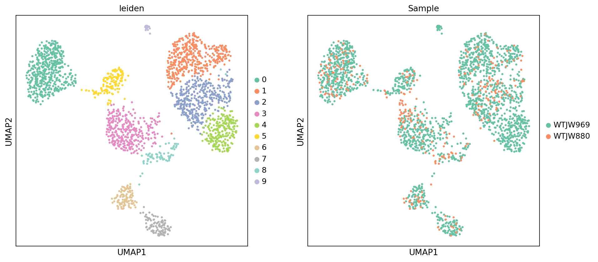
Figure Legend (Methylation UMAP - Cell Type):

The figure below shows the cell distribution of methylation data in UMAP space, colored by cell type (celltype) transferred from RNA data.

• X and Y axes: Two main dimensions after UMAP dimensionality reduction (UMAP_1 and UMAP_2).
• Color: Colors represent cell types transferred from RNA data annotation.
• Points: Each point represents a cell.
• Usage: Evaluate cell type annotation transfer, check distribution patterns of different cell types in methylation space, and verify annotation accuracy.

warnings.filterwarnings('ignore')
sc.set_figure_params(scanpy=True, fontsize=12, facecolor='white', figsize=(6, 6))
sc.pl.umap(adata_met, color = ['celltype'], s=35, palette=my_palette)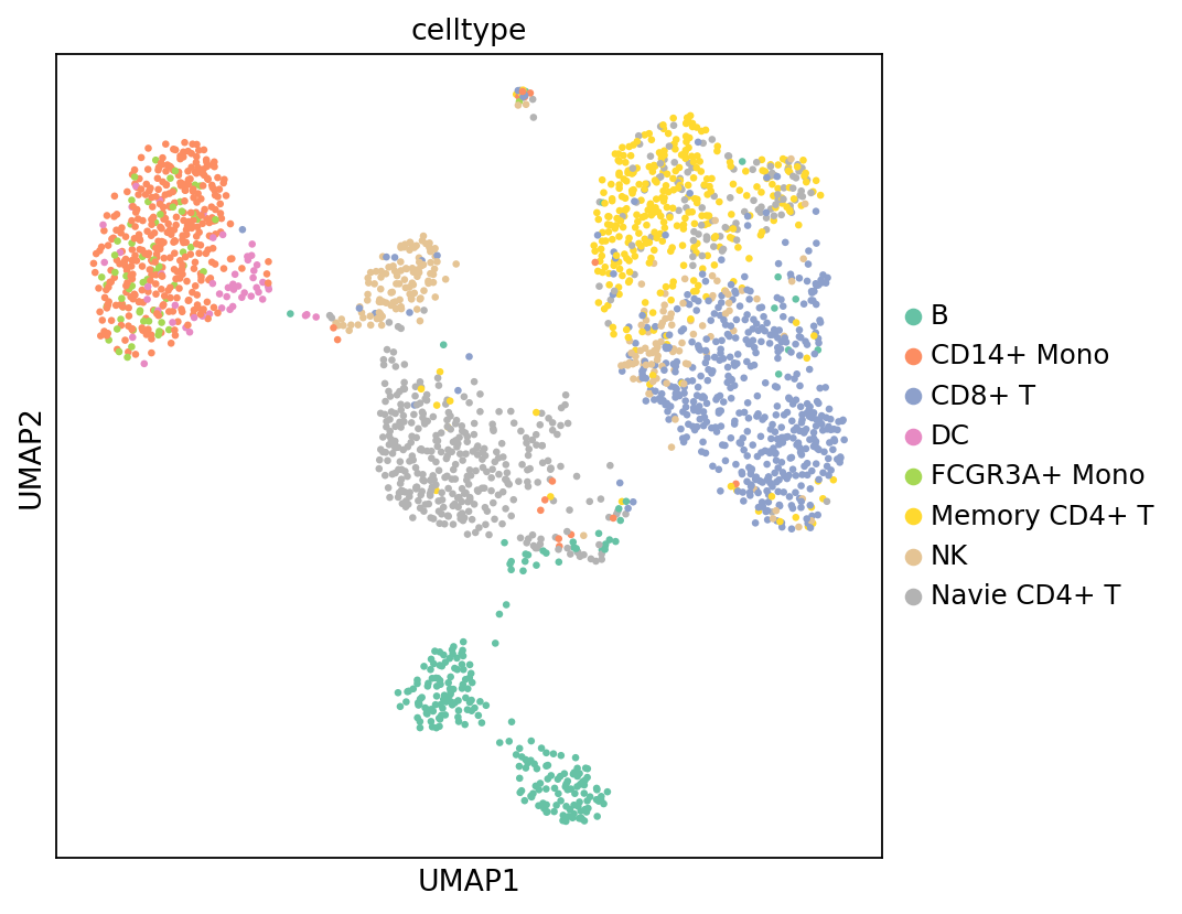

Cell Composition Proportion

Figure Legend (Cell Type Composition Stacked Bar Chart):

The figure below shows the proportional distribution of various cell types (celltype) in different samples (Sample).

• X-axis: Different samples (Sample), facilitating comparison of cell type composition across samples.
• Y-axis: Cell type proportion (0 to 1), representing the percentage of each cell type in the sample.
• Stacked Bar Chart: Each bar represents a sample, colors represent cell types, bar height represents total proportion of all cell types in that sample (100%).
• Color: Colors represent different cell types; legend shows names.
• Usage: Compare cell type composition differences between samples, evaluate sample heterogeneity, and identify sample-specific cell types.

def plot_bar_fraction_data_optimized(adata, x_key, y_key, custom_palette=None):
    # 1. Data Preparation
    df = adata.obs[[x_key, y_key]].copy()
    df[y_key] = df[y_key].astype('category')
    df[x_key] = df[x_key].astype('category')
    
    counts = df.groupby([x_key, y_key]).size().reset_index(name='count')
    totals = counts.groupby(x_key)['count'].transform('sum')
    counts['prop'] = counts['count'] / totals
    prop_pivot = counts.pivot(index=x_key, columns=y_key, values='prop').fillna(0)
    
    clusters = prop_pivot.columns.tolist()    
    bar_colors = None
    
    if f'{y_key}_colors' in adata.uns:
        categories = adata.obs[y_key].cat.categories
        uns_colors = adata.uns[f'{y_key}_colors']
        
        # Prevent color count mismatch
        if len(categories) == len(uns_colors):
            color_dict = dict(zip(categories, uns_colors))
            bar_colors = [color_dict.get(c, '#333333') for c in clusters]
    
    # If color not found above, or logic fails, use custom palette
    if bar_colors is None:
        if custom_palette is None:
            custom_palette = sc.pl.palettes.default_20
        
        # Cyclically assign colors
        bar_colors = [custom_palette[i % len(custom_palette)] for i in range(len(clusters))]

    return prop_pivot, bar_colors

# --- Plotting ---

# Call function, passing your defined my_palette
prop_pivot, bar_colors = plot_bar_fraction_data_optimized(
    adata_met, 
    x_key="Sample", 
    y_key="celltype", 
    custom_palette=my_palette
)

# Set canvas size
plt.rcParams['figure.dpi'] = 100
fig, ax = plt.subplots(figsize=(5, 5)) 
ax.grid(False)
ax.tick_params(axis='both', which='major', labelsize=9)

# Plotting
prop_pivot.plot(
    kind='bar', 
    stacked=True, 
    color=bar_colors, 
    ax=ax, 
    width=0.5,       # Bar width
    edgecolor='none',
    grid=False,
    zorder=3
)

# Beautify axes
ax.set_ylabel('Proportion', fontsize=10)
ax.set_xlabel("")
ax.tick_params(axis='x', rotation=45) # Rotate x-axis labels
ax.spines['top'].set_visible(False)
ax.spines['right'].set_visible(False)

# Beautify legend
ax.legend(
    title='Cell Type', 
    bbox_to_anchor=(1.05, 1), 
    loc='upper left', 
    frameon=False, 
    fontsize=9, 
    title_fontsize=9,
    alignment="left"
)

plt.tight_layout()
plt.show()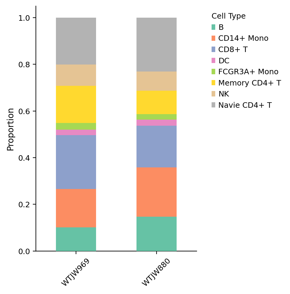

QC Metrics Visualization

This section visualizes QC metric distribution in UMAP space to assess overall data quality and potential anomalies.

Figure Legend (QC Metrics UMAP Distribution):

The figure below shows the distribution of QC metrics in UMAP space, used to evaluate data quality.

• X and Y axes: Two main dimensions after UMAP dimensionality reduction (UMAP_1 and UMAP_2).
• Color: Intensity represents QC metric value; brighter (yellow/white) is higher, darker (black/purple) is lower.
• Visualization Metrics:
  • total_cpg_number (Total CpG Sites): Reflects the total amount of methylation sites captured per cell; higher values indicate better sequencing depth.
  • reads_counts (Sequencing Depth): Reflects sequencing depth per cell; higher values indicate more sequencing data.
  • genome_cov (Genome Coverage): Quantifies the proportion of genomic regions covered by sequencing data; higher values indicate more comprehensive coverage.
  • CpG% (CpG Methylation Rate): Shows overall methylation level of CpG sites, typically in the 0-100% range.
  • CH% (CH Non-CpG Methylation Rate): Reveals modification levels at non-canonical methylation sites; typically < 5% in mammalian cells.
• Points: Each point represents a cell.
• Usage: Identify spatial distribution patterns of QC metrics, detect abnormal cells (e.g., abnormally high/low QC metrics), and evaluate data quality uniformity.

# --- UMAP visualization of QC metrics ---
plt.rcParams['font.size'] = 10         
plt.rcParams['axes.titlesize'] = 10  
# Visualize total_cpg_number, reads_counts, genome_cov, CpG%, CH%
features = ['total_cpg_number', 'reads_counts', 'genome_cov','CpG%', 'CH%']
sc.pl.umap(
    adata_met, 
    color=features, 
    ncols=3,            
    color_map=my_warm_cmap, 
    vmax='p99',         
    s=8,               
    frameon=False,      
    vmin=0,
    show=False 
)

plt.gcf().set_size_inches(10, 5) 
plt.show()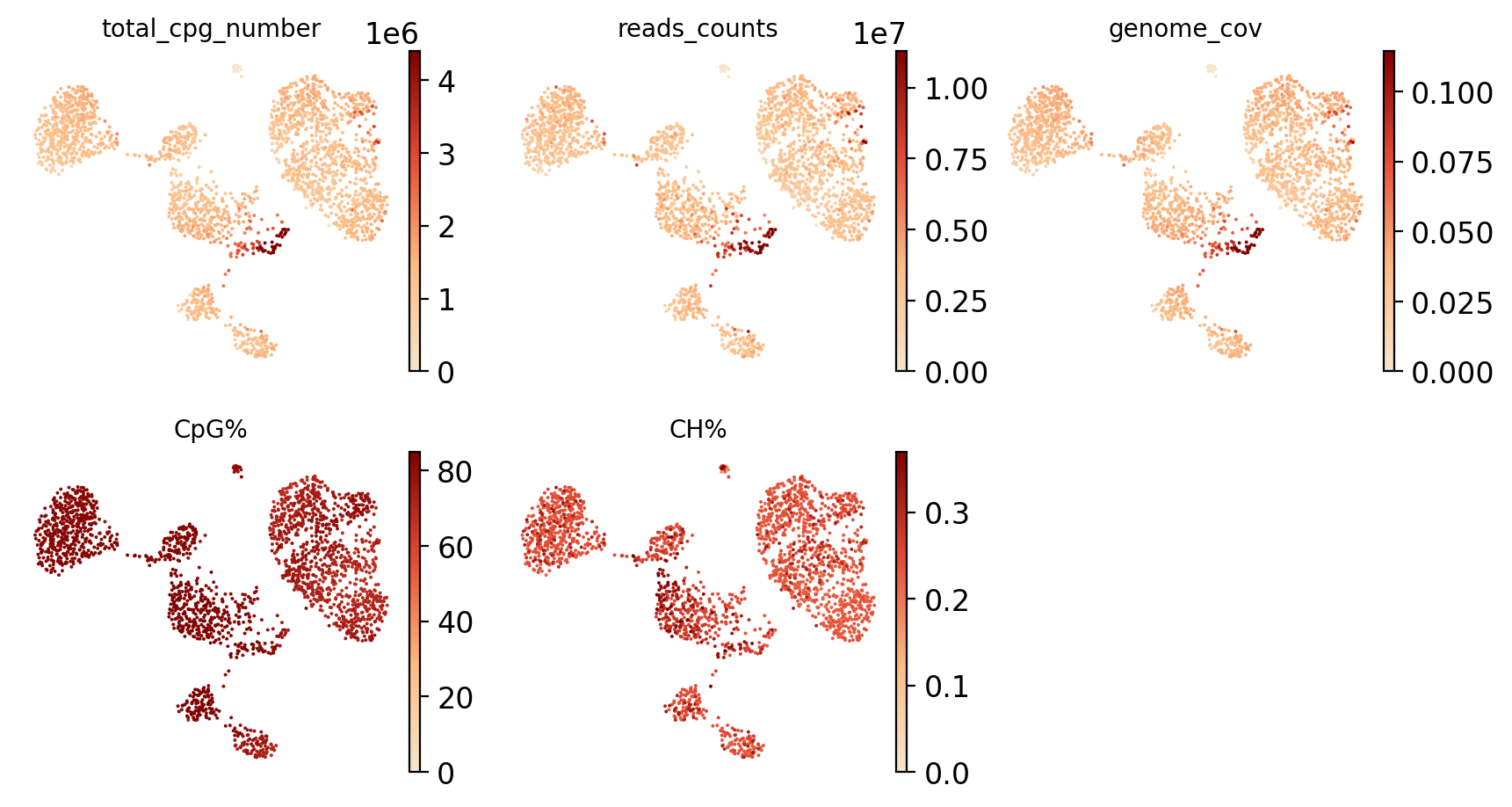

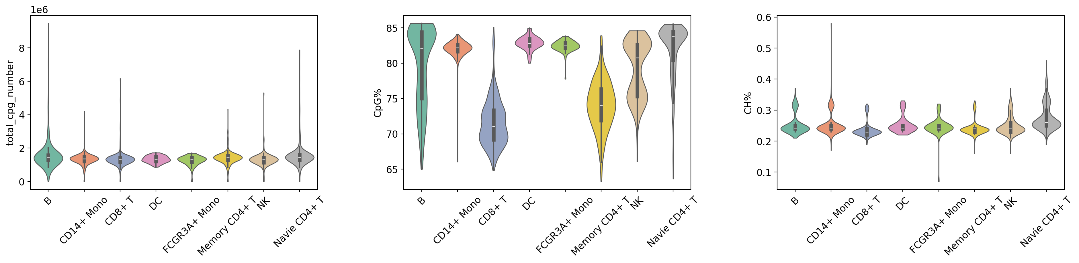
Violin Plot Visualization of QC Metrics

This section uses violin plots to display the distribution of QC metrics across different cell groups (Leiden clusters and cell types) to assess data quality consistency across cell populations.

Figure Legend (QC Metrics Violin Plot):

The figure below shows the distribution characteristics of QC metrics in different cell groups (Leiden clusters and cell types).

• X-axis: Different cell groups, including Leiden clusters (leiden) and cell types (celltype), facilitating comparison of QC metrics across groups.
• Y-axis: Values of QC metrics, including total_cpg_number, CpG%, and CH%.
• Violin Plot: Each violin represents a cell group; width indicates cell density in that value range (wider = more cells). Includes a box plot showing median, quartiles, and outliers.
• Grouping Method:
  • Group by Leiden Clusters: Displays differences in QC metrics between clusters to evaluate clustering quality.
  • Group by Cell Type: Displays differences in QC metrics between cell types to evaluate the rationality of cell type annotation.
• Usage: Evaluate data quality uniformity across cell groups, identify groups with abnormal QC metrics, and verify reliability of clustering and annotation.

warnings.filterwarnings('ignore')
plt.rcParams['figure.figsize'] = (6, 4)
plt.rcParams['axes.grid'] = False

violin_params = {
    'palette': my_palette,   
    'stripplot': False,      
    'inner': 'box',          
    'linewidth': 1,        
    'size': 1,               
    'cut': 0, 
    'multi_panel': True      
}

print("\n=== 质控指标分布 (按 Cluster) ===")
# Group by leiden clustering
sc.pl.violin(
    adata_met, 
    keys=['total_cpg_number', 'CpG%', 'CH%'], 
    groupby='leiden', 
    **violin_params  
)
plt.show()

print("\n=== 质控指标分布 (按 Cell Type) ===")
# Group by cell type (with rotation)
sc.pl.violin(
    adata_met, 
    keys=['total_cpg_number', 'CpG%', 'CH%'], 
    groupby='celltype', 
    rotation=45,     
    **violin_params
)
plt.show()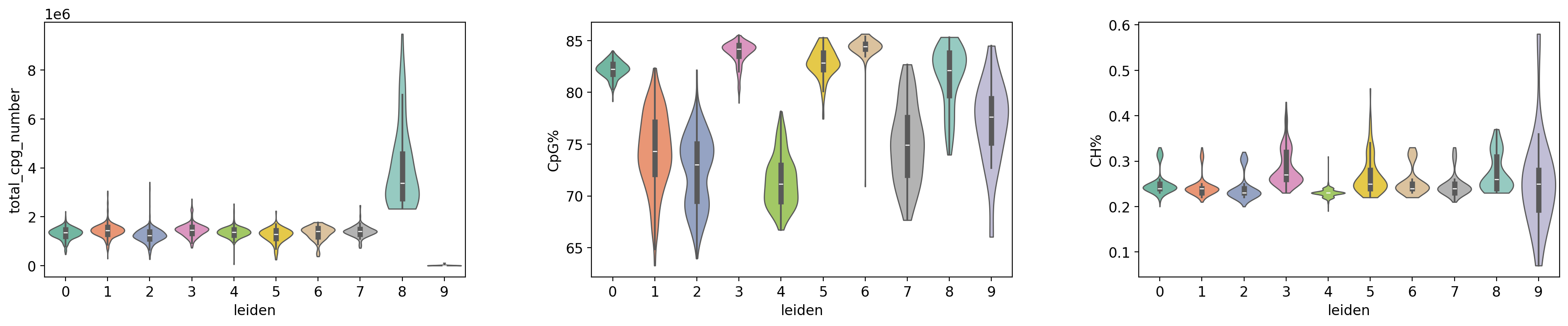

output

=== 质控指标分布 (按 Cluster) ===

=== 质控指标分布 (按 Cell Type) ===

adata_met.write_h5ad('adata_met.h5ad')