scMethyl + RNA Multi-omics: CNV Copy Number Variation Analysis (Based on CopyKit)

Author: SeekGene

Time: 33 min

Words: 6.5k words

Updated: 2026-03-05

Reads: 0 times

scMethyl + RNA-seq Analysis Guide Notebooks

Module Introduction

This module is based on CopyKit (v0.1.3), designed for inferring genome-wide Copy Number Variations (CNV) from single-cell sequencing data.

CopyKit is a powerful R language toolkit capable of systematic preprocessing, normalization, segmentation, and clustering analysis of single-cell data. By detecting genome-wide coverage changes, it achieves the following core analysis goals:

Variation Detection: Precisely locates chromosome amplification and deletion events in tumor cells to map the genome-wide CNV profile.
Cell Classification: Effectively distinguishes normal cells (diploid) from tumor cells (non-diploid/aneuploid) based on CNV features.
Clonal Evolution: Explore intra-tumor heterogeneity and clonal evolution trajectories through subclonal structure reconstruction.

Note: This analysis is mainly applicable to Human Tumor Samples, relying on human reference genomes (hg19/hg38) for alignment and annotation.

Input File Preparation

This module supports two types of input files; please choose according to your data processing stage:

Option A: Import Analyzed Results Directly (Recommended)

If you have previously run the CopyKit runVarbin workflow, you can directly use the generated .rds file. This is the fastest method.

File Structure Example:

text

workspace/data/AY1768876207519/methylation/demo3MDA-task-2/MDA_cs/cnvPreflight/
├── copykit_MDA_cs_1Mb.rds      # 1Mb Resolution Results
├── copykit_MDA_cs_500kb.rds    # 500kb Resolution Results
└── copykit_MDA_cs_220kb.rds    # 220kb Resolution Results

Option B: Start from Single-cell BAM Files

If you have split single-cell BAM files, they can be used directly as input.

Note: Input BAM files must undergo Flag Correction and Deduplication processing to ensure quantitative accuracy.

File Structure Example:

text

./
├── AAAGAAGAAGAGTTTAG.dedup.bam
├── AAAGAAGAAGGAGTGGT.dedup.bam
├── ...
└── TTTGGATATTTGTGAGG.dedup.bam

Detailed Tutorial: For a complete guide on generating the standard single-cell BAM files mentioned above (including splitting, Flag correction, deduplication), please refer to: guide

CopyKit Analysis Pipeline

Key Parameter Settings

During analysis, the following three parameters are crucial for data quality control and result resolution:

Parameter Name	Chinese Meaning	Default Value	Detailed Description
`bin_sizes`	Genomic Window Size	220kb, 500kb, 1Mb	Determines CNV analysis resolution. • Smaller (e.g. 220kb): Higher resolution, detects smaller variants, requires higher depth, more noise. • Larger (e.g. 1Mb): Smoother data, lower noise, only detects large variants. Note: Changing this requires re-running `runVarbin` (input BAM, time-consuming).
`min_bincount`	Min Reads Abundance	10	QC Parameter. Requires avg Reads per Bin > this value. Removes low-quality cells with insufficient depth for accurate CNV inference.
`pearson_corr_cutoff`	Pearson Correlation Filter Threshold	0.8 (Default 0.9)	QC Parameter (Do not confuse with `bin_size`). CopyKit calculates Pearson correlation of each cell with its nearest neighbors (k=5). If correlation is below this threshold, the cell is considered an "outlier" or low quality and filtered. • Increasing this value yields purer clones but may lose some heterogeneous cells.

Best Practice Recommendations

Choice of bin_sizes: * This module calculates 220kb, 500kb, and 1Mb resolutions simultaneously by default. * Resolutions supported by CopyKit: 55kb, 110kb, 195kb, 220kb, 280kb, 500kb, 1Mb, 2.8Mb. * Strategy: If the sample sequencing depth is low, it is recommended to prioritize 1Mb or 500kb results; when the depth is high, 220kb can be used to obtain finer results. * CopyKit has internally preset and optimized these Bin regions, filtering out repetitive sequences and difficult-to-align regions.
About Filtering Parameters (min_bincount & resolution): * If too few cells are retained, min_bincount can be appropriately lowered (e.g., to 5), but this will increase noise. * If the clustering result contains many messy single cells, the pearson_corr_cutoff threshold can be appropriately raised (e.g., to 0.9).

library(copykit)
library(BiocParallel)
library(ggplot2)
# --- Input parameter configuration ---

## genome_version: Reference genome version used for data alignment
genome_version <- 'hg38'

## outdir: Result output directory
outdir <- '/PROJ2/FLOAT/weiqiuxia/project/20241227_methy/script/standard_reports/modules/copykit/test/results/MDA_cs'

## bam_dir: Directory containing single-cell BAM files (Option B)
bam_dir <- NULL

## rds_path: Directory of generated RDS files (Option A)
rds_path <- '/PROJ2/FLOAT/weiqiuxia/project/20241227_methy/script/standard_reports/modules/copykit/test/input/MDA_cs/'

## samplename: Sample name identifier
samplename <- 'MDA_cs'

## min_bincount: Minimum average Reads count filtering threshold
# Used to filter out low-quality cells with low Read Counts, recommended to keep default value
min_bincount <- 10

## bin_sizes: Analysis resolution list
bin_sizes <- c('220kb', '500kb', '1Mb')

## pearson_corr_cutoff: Correlation filtering threshold (for findOutliers)
pearson_corr_cutoff <- 0.8

## is_paired_end: Whether it is paired-end sequencing (TRUE/FALSE)
is_paired_end <- TRUE

## remove_Y: Whether to remove Y chromosome (TRUE/FALSE)
remove_Y <- TRUE

## threads: Parallel calculation thread count
threads <- 8

## skipKNNSmooth: Whether to skip KNNSmooth (TRUE/FALSE)
skipKNNSmooth <- FALSE

dir.create(outdir, recursive = TRUE)

plotConsensusLine_static <- function(scCNA, sample) {

    # bindings for NSE
    start <- xstart <- xend <- abspos <- NULL

    ####################
    ## checks
    ####################
    if (nrow(consensus(scCNA)) == 0) {
        stop("Slot consensus is empty. Run calcConsensus()")
    }

    ####################
    ## aesthetic setup
    ####################

    # obtaining chromosome lengths
    chr_ranges <-
        as.data.frame(SummarizedExperiment::rowRanges(scCNA))
    chr_lengths <- rle(as.numeric(chr_ranges$seqnames))$lengths

    # obtaining first and last row of each chr
    chr_ranges_start <- chr_ranges %>%
        dplyr::group_by(seqnames) %>%
        dplyr::arrange(seqnames, start) %>%
        dplyr::filter(dplyr::row_number() == 1) %>%
        dplyr::ungroup()

    chr_ranges_end <- chr_ranges %>%
        dplyr::group_by(seqnames) %>%
        dplyr::arrange(seqnames, start) %>%
        dplyr::filter(dplyr::row_number() == dplyr::n()) %>%
        dplyr::ungroup()

    # Creating data frame object for chromosome rectangles shadows
    chrom_rects <- data.frame(
        chr = chr_ranges_start$seqnames,
        xstart = as.numeric(chr_ranges_start$abspos),
        xend = as.numeric(chr_ranges_end$abspos)
    )
    xbreaks <- rowMeans(chrom_rects %>%
        dplyr::select(
            xstart,
            xend
        ))

    if (nrow(chrom_rects) == 24) {
        chrom_rects$colors <- rep(
            c("white", "gray"),
            length(chr_lengths) / 2
        )
    } else {
        chrom_rects$colors <- c(rep(
            c("white", "gray"),
            (length(chr_lengths) / 2)
        ), "white")
    }

    # Creating the geom_rect object
    ggchr_back <-
        list(geom_rect(
            data = chrom_rects,
            aes(
                xmin = xstart,
                xmax = xend,
                ymin = -Inf,
                ymax = Inf,
                fill = colors
            ),
            alpha = .2
        ), scale_fill_identity())

    sec_breaks <- c(0, 0.5e9, 1e9, 1.5e9, 2e9, 2.5e9, 3e9)
    sec_labels <- c(0, 0.5, 1, 1.5, 2, 2.5, 3)


    # theme
    ggaes <- list(
        scale_x_continuous(
            breaks = xbreaks,
            labels = gsub("chr", "", chrom_rects$chr),
            position = "top",
            expand = c(0, 0),
            sec.axis = sec_axis(
                ~.,
                breaks = sec_breaks,
                labels = sec_labels,
                name = "genome position (Gb)"
            )
        ),
        theme_classic(),
        theme(
            axis.text.x = element_text(
                angle = 0,
                vjust = .5,
                size = 15
            ),
            axis.text.y = element_text(size = 15),
            panel.border = element_rect(
                colour = "black",
                fill = NA,
                size = 1.3
            ),
            legend.position = "top",
            axis.ticks.x = element_blank(),
            axis.title = element_text(size = 15),
            plot.title = element_text(size = 15)
        )
    )
    ####################
    # obtaining and wrangling data
    ####################


    con <- consensus(scCNA)

    con_l <- con %>%
        dplyr::mutate(abspos = chr_ranges$abspos) %>%
        tidyr::gather(
            key = "group",
            value = "segment_ratio",
            -abspos
        )

    choice <- gtools::mixedsort(unique(con_l$group))
    
    df_plot <- con_l %>% dplyr::filter(group %in% sample)

    p <- ggplot(df_plot) +
        ggchr_back +
        ggaes +
        geom_line(aes(abspos, segment_ratio, color = group),size = 1.2, alpha = .7) +
    labs(
        x = "",
        y = "consensus segment ratio"
    )

    return(p)
}

# Set parallel parameters
register(MulticoreParam(progressbar = T, workers = threads), default = T)

# --- Input path logic judgment ---
# Prioritize reading data under rds_path; if not found, try reading bam_dir
bam_flag <- FALSE
if(!is.null(bam_dir) & !is.null(rds_path)){
    if(!dir.exists(rds_path)){
        if(!dir.exists(bam_dir)){
            stop("Error: Both bam_dir and rds_path do not exist!")
        }else{
            input_dir <- bam_dir
            bam_flag <- TRUE
        }
    }else{
        input_dir <- rds_path
    }
} else if(is.null(bam_dir) & !is.null(rds_path)){
    input_dir <- rds_path
} else if(!is.null(bam_dir) & is.null(rds_path)){
    input_dir <- bam_dir
    bam_flag <- TRUE
} else{
    stop("Error: Please set either bam_dir or rds_path!")
}

# --- Genome version identification ---
if(length(grep('(GRCh38)|(hg38)', genome_version, ignore.case = TRUE )) > 0){
    genome <- 'hg38'
}else if(length(grep('(GRCh37)|(hg19)', genome_version, ignore.case = TRUE )) > 0){
    genome <- 'hg19'
}else{
    stop('Error: Cannot recognize genome version. Please use hg38, GRCh38, hg19, or GRCh37.')
}

# --- Run runVarbin (if input is BAM) ---
if(bam_flag){
   for(i in bin_sizes){
        message(paste("Processing bin size:", i))
        tumor <- runVarbin(input_dir, 
                        min_bincount = min_bincount,
                        remove_Y = remove_Y,
                        is_paired_end = is_paired_end,
                        resolution = i,
                        genome = genome)
        saveRDS(tumor, paste0(outdir, '/copykit_', samplename, '_', i, '.rds'))
    }
    input_dir <- outdir
}

Data Preprocessing Principle

CopyKit uses the core function runVarbin to preprocess input BAM files. This process includes the following key modules:

runCountReads (Bin Counting): * Bin Counting: Based on preset genomic windows (Bins), use featureCounts to count the number of Reads falling within each Bin. * Deduplication: Reads marked as PCR Duplicates are automatically ignored during counting. * Paired-end processing: If is_paired_end = TRUE, paired-end Reads are counted as one Fragment. * Filtering: Default removal of Y chromosome regions (optional), and exclusion of low-quality cells with low average Read Counts based on counting results. * GC Correction: Theoretically sequencing depth should be uniformly distributed, but high GC content regions often have PCR amplification bias, leading to a positive correlation between fragment counts and GC content. Before CNV analysis, the algorithm performs GC bias correction for each cell, pulling counts affected by GC back to the baseline to eliminate systematic errors.
runVst (Variance Stabilizing Transformation): * Principle: Bin Counts in single-cell DNA sequencing usually follow a Poisson Distribution, characterized by variance equal to the mean. This causes noise in high-abundance regions to be much larger than in low-abundance regions. * Function: Use Freeman-Tukey (FT) transformation to convert data to an approximate normal distribution. The transformed data variance is approximately constant at 1 and no longer depends on the mean. This step is crucial for accurate breakpoint detection (Segmentation).
runSegmentation (CBS Segmentation): * Smoothing: First use a smoothing algorithm to trim extremely rare "spike" values that are much higher or lower than adjacent Bins to reduce noise interference. * CBS Algorithm: Run Circular Binary Segmentation (CBS) algorithm for each cell to find breakpoints where copy number changes on the genome. * Merging: Merge consecutive Bins with similar counts on the genome into Segments. All Bins within the same Segment have the same Segment Ratio. * Segment Ratio Meaning (Relative to average ploidy): * 1.0: Diploid state (Diploid). * 1.5: 3 copies (Gain). * 0.5: Single copy loss (Loss). * 2.0: 4 copies amplification (Amplification).
logNorm (Log Normalization): * Perform Log transformation on Segment Ratio to generate logr matrix, facilitating subsequent UMAP dimensionality reduction and clustering analysis.

Matrix generated after running runVarbin (Bin x Cells):

bincounts: Raw Read Counts matrix after GC correction.
ft: Numerical matrix after Variance Stabilizing Transformation (VST), used as input for the segmentation algorithm.
smoothed_bincounts: Smoothed counts after removing outliers, used for absolute copy number inference.
segment_ratios: Ratio matrix after segmentation, core data for cell filtering, plotting, clustering, and CNV analysis.
ratios: Normalized ratio matrix based on smoothed_bincounts.
logr: Log-transformed Segment Ratio.

The above matrix can be accessed via assay(tumor_list[['220kb']], 'bincounts').

varbin_rds <- list.files(rds_path,pattern = '.rds', full.names = T)

Quality Control

The runMetrics function calculates Overdispersion for each cell based on bincounts, and we also visualize Total Reads, Reads Assigned to Bins, and Breakpoints Count for each cell.

Key QC Metrics

Overdispersion: * Reflects sequencing coverage uniformity. Theoretically, Read Counts of adjacent Bins should be similar. * If Overdispersion value is too high, it indicates large differences between adjacent Bins and obvious technical noise, which may affect CNV result accuracy.
Breakpoint Count: * Normal diploid cells, or cells without variation, usually have a Breakpoint Count close to 0. * Tumor cells usually have higher breakpoint counts due to genomic instability.
Total Reads: * The number of Reads per cell can reflect whether the data amount for each cell is sufficient.
Reads Assigned bins: * Valid Reads count. If this value is too low, it indicates that many Reads aligned to repetitive sequences or low-quality regions (CopyKit preset Bins have filtered these regions), suggesting poor cell sequencing quality.

CopyKit Recommendation: Typically, a sequencing depth of 1M reads/cell and a duplication rate of ~10% are sufficient to obtain high-quality 220kb resolution CNV results.

Below shows the distribution of QC metrics at different resolutions:

Figure Legend: The figure below shows the distribution of four QC metrics.
X-axis: Sample.
Y-axis: Specific values of each metric.
Color: Represents overdispersion magnitude; brighter color means higher data noise.
Interpretation: High-quality data typically exhibits higher reads_assigned_bins and lower overdispersion.

tumor_list <- list()
for(i in varbin_rds){
    bin_size_name <- gsub('.*_(\\d+[Mk]b).rds','\\1',i)
    tumor_list[[bin_size_name]] <- readRDS(i)
    tumor_list[[bin_size_name]] <- runMetrics(tumor_list[[bin_size_name]])   
}

output

Calculating overdispersion.

|======================================================================| 100%

Counting breakpoints.

Done.

Calculating overdispersion.

|======================================================================| 100%

Counting breakpoints.

Done.

Calculating overdispersion.

|======================================================================| 100%

Counting breakpoints.

Done.

options(repr.plot.width = 8, repr.plot.height = 7, repr.plot.res = 150)
pic <- plotMetrics(
    tumor_list[['220kb']],
    metric = c(
        "reads_total",
        "reads_assigned_bins",
        "overdispersion", 
        "breakpoint_count"), 
    label = 'overdispersion') +
ggtitle('220kb Metrics') +
theme(plot.title = element_text(hjust = .5, size = 20))
pic
ggsave(filename = file.path(outdir, paste0('plotMetrics_',samplename, '_220kb.pdf')), pic, width = 8, height = 7)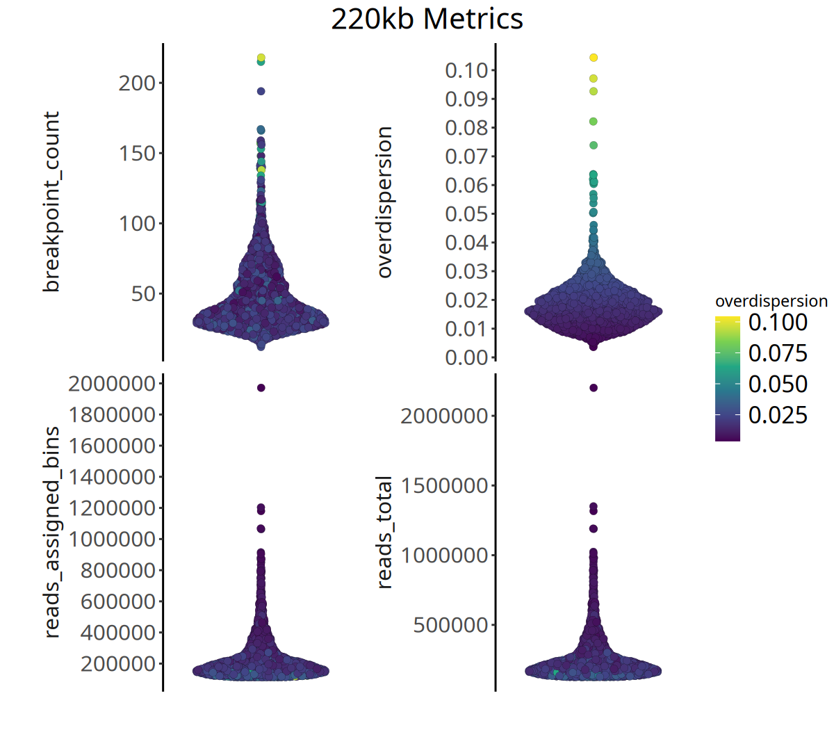

output

Coloring by: overdispersion

options(repr.plot.width = 8, repr.plot.height = 7, repr.plot.res = 150)
pic <- plotMetrics(
    tumor_list[['500kb']],
    metric = c(
        "reads_total",
        "reads_assigned_bins",
        "overdispersion", 
        "breakpoint_count"), 
    label = 'overdispersion') +
ggtitle('500kb Metrics') +
theme(plot.title = element_text(hjust = .5, size = 20))

pic
ggsave(filename = file.path(outdir, paste0('plotMetrics_',samplename, '_500kb.pdf')), pic, width = 8, height = 7)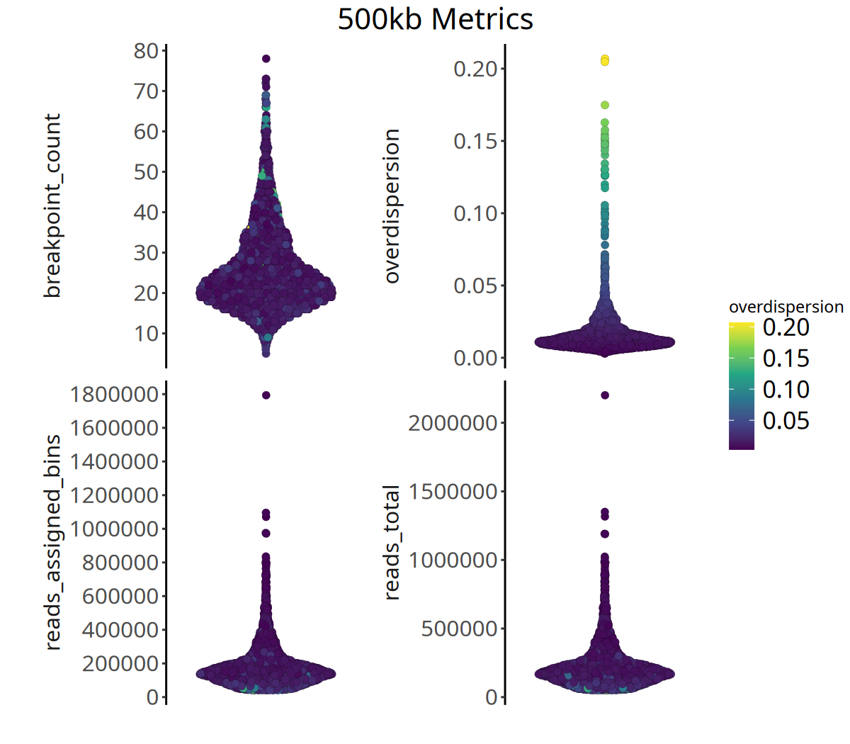

output

Coloring by: overdispersion

options(repr.plot.width = 8, repr.plot.height = 7, repr.plot.res = 150)
pic <- plotMetrics(
    tumor_list[['1Mb']],
    metric = c(
        "reads_total",
        "reads_assigned_bins",
        "overdispersion", 
        "breakpoint_count"), 
    label = 'overdispersion') +
ggtitle('1Mb Metrics') +
theme(plot.title = ggplot2::element_text(hjust = .5, size = 20))

pic
ggsave(filename = file.path(outdir, paste0('plotMetrics_',samplename, '_1Mb.pdf')), pic, width = 8, height = 7)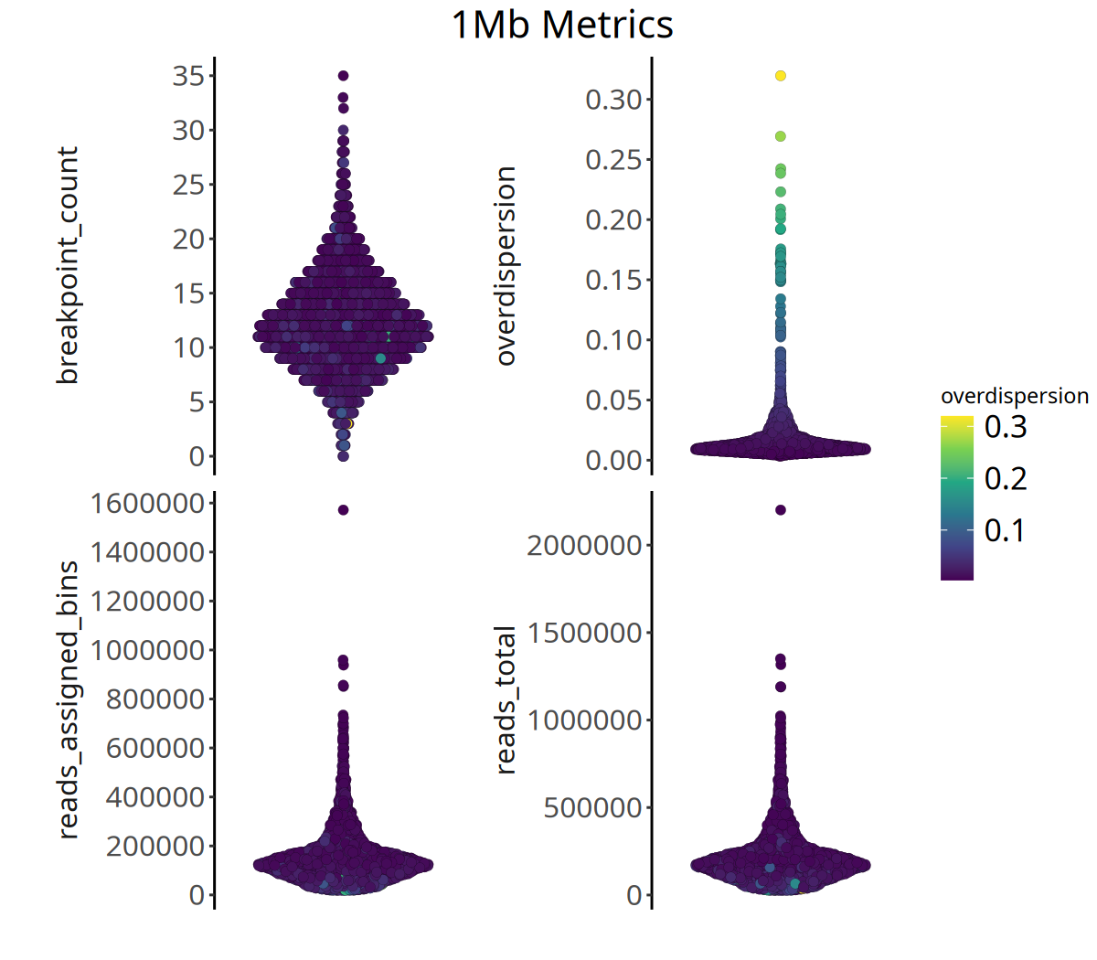

output

Coloring by: overdispersion

Normal Diploid Cell Filtering

Before clonal evolution analysis, clustering, and lineage tree construction, normal diploid cells must be removed. If retained, they cluster into a large "fake clone", severely interfering with tumor heterogeneity resolution.

The findAneuploidCells function is used to distinguish normal cells from aneuploid (tumor) cells:

Judgment Criteria: Segment Ratios of normal diploid cells should be a flat straight line, with a coefficient of variation (CV = SD / Mean) close to 0.
Tumor Cells: Due to numerous amplifications and deletions, their Segment Ratios have larger standard deviations and higher CV values.
Bimodal Distribution: CV distribution of normal and tumor cells typically presents a bimodal pattern. If a cell's CV fluctuation exceeds 5 times the diploid background noise, it is determined as Aneuploid.

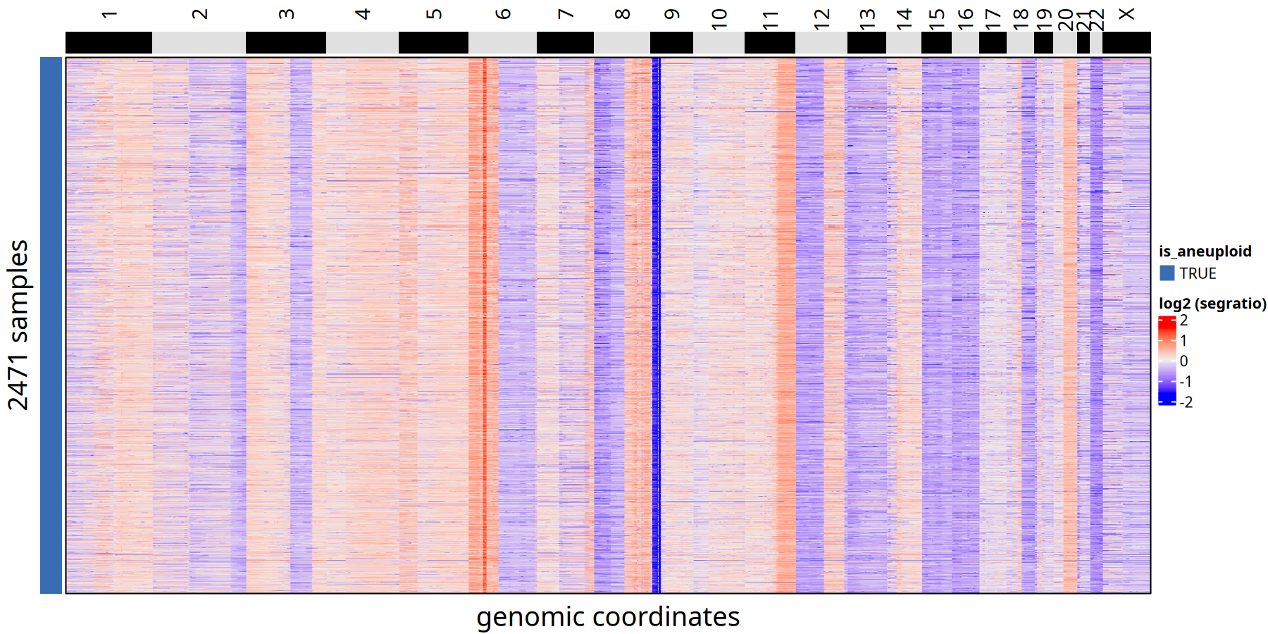
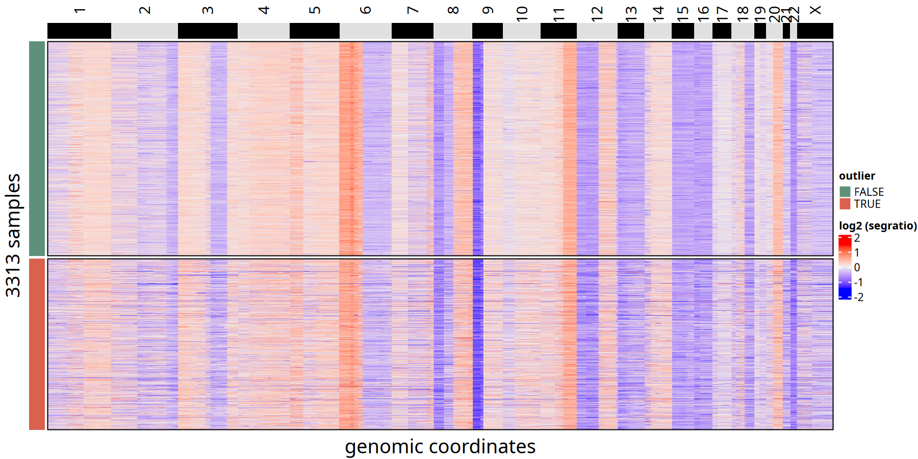
CNV results for diploid and aneuploid at 220kb bin

Legend Explanation: In the heatmap below, each column represents a genomic Bin (sorted by position), and each row represents a cell.
Left Color Bar (is_aneuploid): TRUE indicates aneuploid (tumor) cells, FALSE indicates normal diploid cells.
Heatmap Colors: Represent Log2 transformed Segment Ratio. Red indicates copy number gain/amplification, blue indicates loss/deletion, white indicates diploid state (Neutral).

options(repr.plot.width = 12, repr.plot.height = 6, repr.plot.res = 150)
suppressMessages({
    tumor_list[['220kb']] <- findAneuploidCells(tumor_list[['220kb']])
    ht <- plotHeatmap(
        tumor_list[['220kb']], 
        label = 'is_aneuploid', 
        row_split = 'is_aneuploid', 
        n_threads = threads)
    ht
})
pdf(file.path(outdir, paste0('plotHeatmap_', samplename, '_220k_aneuploid.pdf')), width = 12, height = 6)
ht
dev.off()

output

number of iterations= 6

pdf: 2

CNV Results for Diploid and Aneuploid at 500kb bin

options(repr.plot.width = 12, repr.plot.height = 6, repr.plot.res = 150)
suppressMessages({
    tumor_list[['500kb']] <- findAneuploidCells(tumor_list[['500kb']])
    ht <- plotHeatmap(tumor_list[['500kb']], label = 'is_aneuploid', row_split = 'is_aneuploid', n_threads = threads)
})
pdf(file.path(outdir, paste0('plotHeatmap_', samplename, '_500k_aneuploid.pdf')), width = 12, height = 6)
ht
dev.off()

output

number of iterations= 7

pdf: 2

CNV results for diploid and aneuploid at 1Mb bin

options(repr.plot.width = 12, repr.plot.height = 6, repr.plot.res = 150)
suppressMessages({
    tumor_list[['1Mb']] <- findAneuploidCells(tumor_list[['1Mb']])
    ht <- plotHeatmap(tumor_list[['1Mb']], label = 'is_aneuploid', row_split = 'is_aneuploid', n_threads = threads)
})

pdf(file.path(outdir, paste0('plotHeatmap_', samplename, '_1Mb_aneuploid.pdf')), width = 12, height = 6)
ht
dev.off()

output

number of iterations= 8

pdf: 2

# Filter out normal diploid cells
for(i in names(tumor_list)){
    tumor_list[[i]] <- tumor_list[[i]][,colData(tumor_list[[i]])$is_aneuploid == TRUE]
}

Outlier Cell Filtering

To build accurate tumor subclonal and evolutionary relationships, we need to further use findOutliers to remove cells with extremely low correlation to other cells, which may be technical noise or poor quality.

This step uses Pearson correlation as the metric. If a cell's average correlation with its K nearest neighbors is below pearson_corr_cutoff (default 0.9, set to 0.8 in this tutorial), it is flagged as outlier.

for(i in names(tumor_list)){
    tumor_list[[i]] <- findOutliers(tumor_list[[i]], resolution = pearson_corr_cutoff)
}

output

Calculating correlation matrix.

|======================================================================| 100%

Marked 1469 cells as outliers.

Adding information to metadata. Access with colData(scCNA).

Done.

Calculating correlation matrix.

|======================================================================| 100%

Marked 1144 cells as outliers.

Adding information to metadata. Access with colData(scCNA).

Done.

Calculating correlation matrix.

|======================================================================| 100%

Marked 1493 cells as outliers.

Adding information to metadata. Access with colData(scCNA).

Done.

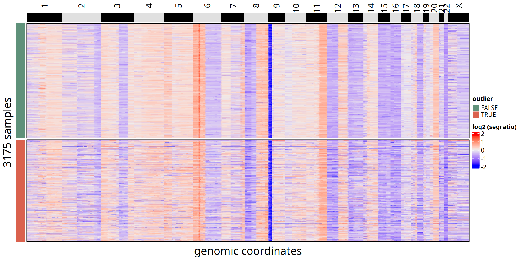
CNV Heatmap Comparison between Outliers and Retained Cells at 220kb Resolution

Figure Legend: Outlier Cell Identification Heatmap.
Left Color Bar (outlier): TRUE (red) represents low-quality cells identified as outliers; FALSE (blue) represents retained high-quality tumor cells.
Features: Outlier cells usually show chaotic signals or copy number patterns distinct from other tumor cells.

options(repr.plot.width = 12, repr.plot.height = 6, repr.plot.res = 150)
suppressMessages({
    ht <- plotHeatmap(tumor_list[['220kb']], label = 'outlier', row_split = 'outlier', n_threads = threads)
    ht
})

pdf(file.path(outdir, paste0('plotHeatmap_', samplename, '_220kb_outlier.pdf')), width = 12, height = 6)
ht
dev.off()
tumor_list[['220kb']] <- tumor_list[['220kb']][,colData(tumor_list[['220kb']])$outlier == FALSE]

pdf: 2

CNV Heatmap Comparison of Outlier vs Retained Cells at 500kb Resolution

options(repr.plot.width = 12, repr.plot.height = 6, repr.plot.res = 150)
suppressMessages({
    ht <- plotHeatmap(tumor_list[['500kb']], label = 'outlier', row_split = 'outlier', n_threads = threads)
    ht
})
pdf(file.path(outdir, paste0('plotHeatmap_', samplename, '_500kb_outlier.pdf')), width = 12, height = 6)
ht
dev.off()
tumor_list[['500kb']] <- tumor_list[['500kb']][,colData(tumor_list[['500kb']])$outlier == FALSE]

pdf: 2

CNV Heatmap Comparison between Outliers and Retained Cells at 1Mb Resolution

options(repr.plot.width = 12, repr.plot.height = 6, repr.plot.res = 150)
suppressMessages({
    ht <- plotHeatmap(tumor_list[['1Mb']], label = 'outlier', row_split = 'outlier', n_threads = threads)
    ht
})
pdf(file.path(outdir, paste0('plotHeatmap_', samplename, '_1Mbkb_outlier.pdf')), width = 12, height = 6)
ht
dev.off()
tumor_list[['1Mb']] <- tumor_list[['1Mb']][,colData(tumor_list[['1Mb']])$outlier == FALSE]

pdf: 2

KNN Smoothing

Due to extremely low single-cell sequencing depth (high sparsity), raw Bin Counts data is often noisy. The knnSmooth function uses the K-Nearest Neighbors (KNN) algorithm to enhance signals and significantly reduce random noise by integrating information from each cell and its k most similar neighbors (default k=4).

Parameter Tuning: If data coverage is extremely low, k value can be increased appropriately, but excessively large k may blur subtle differences between subclones. If you find too many clusters subsequently, try skipping the knnSmooth step.

if(skipKNNSmooth){
    for(i in names(tumor_list)){
        suppressMessages({tumor_list[[i]] <- knnSmooth(tumor_list[[i]], k = 4)})
    }
    saveRDS(tumor_list, file.path(outdir, paste0(samplename, '_copykit_analysis.rds')))
}

Clustering Analysis and Subclonal Evolution Analysis

Dimensionality Reduction

To visually display the clonal structure of tumor cells on a 2D plane, we use the UMAP (Uniform Manifold Approximation and Projection) algorithm to reduce the dimensionality of high-dimensional copy number data (logr matrix).

Meaning: In UMAP space, each point represents a cell. Distances between points reflect the similarity of their genome-wide copy number profiles. Cells clustered together usually represent Subclones with the same CNV characteristics.

for(i in names(tumor_list)){
    tumor_list[[i]] <- runUmap(tumor_list[[i]])
}

output

Using assay: logr

Embedding data with UMAP. Using seed 17

Access reduced dimensions slot with: reducedDim(scCNA, 'umap').

Done.

Using assay: logr

Embedding data with UMAP. Using seed 17

Access reduced dimensions slot with: reducedDim(scCNA, 'umap').

Done.

Using assay: logr

Embedding data with UMAP. Using seed 17

Access reduced dimensions slot with: reducedDim(scCNA, 'umap').

Done.

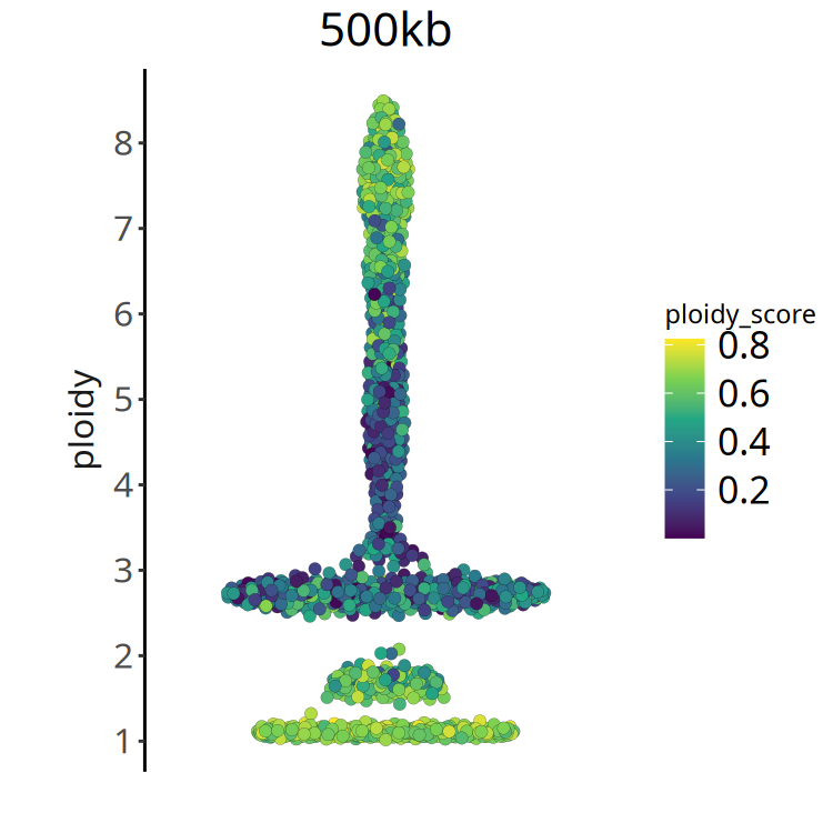
Absolute Ploidy Inference

The calcInteger function uses the scquantum algorithm to convert Relative Copy Number Ratios into Absolute Integer Copy Numbers. This is because biological copy numbers must be integers (e.g., 2, 3, 4).

Ploidy Score: This metric measures the quality of integer fitting. * Score close to 0: Good fitting effect, clear CNV status of cells, easy to judge whether it is 2 copies or 3 copies. * High score: Indicates noisy data, difficult to accurately judge its absolute copy number.
Recommendation: In subsequent analysis, refer to ploidy score to further exclude cells with extremely poor fitting quality.

for(i in names(tumor_list)){
    tumor_list[[i]] <- calcInteger(tumor_list[[i]], method = 'scquantum', assay = 'smoothed_bincounts')
}

output

|======================================================================| 100%

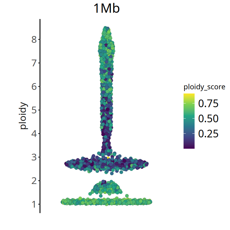
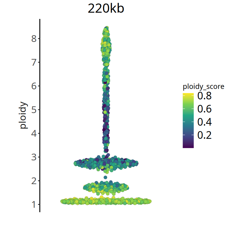
Figure Legend: Ploidy Score Distribution.
X-axis: Cell ordering.
Y-axis: Ploidy Score.
Color: Darker color (smaller value) indicates more reliable ploidy inference. If most cells have large ploidy scores, it suggests poor sample quality or complex heterogeneity.

options(repr.plot.width = 5, repr.plot.height = 5)
for(i in names(tumor_list)){
    
    suppressMessages({
        pic <- plotMetrics(
            tumor_list[[i]], 
            metric = 'ploidy', 
            label = 'ploidy_score') + 
        ggtitle(i) + 
        theme(plot.title = element_text(hjust = .5, size = 20))
    })
    print(pic)
    ggsave(file.path(outdir, paste0('ploidy_score_',samplename,'_',i,'.pdf')), pic, width = 5, height = 5)
}

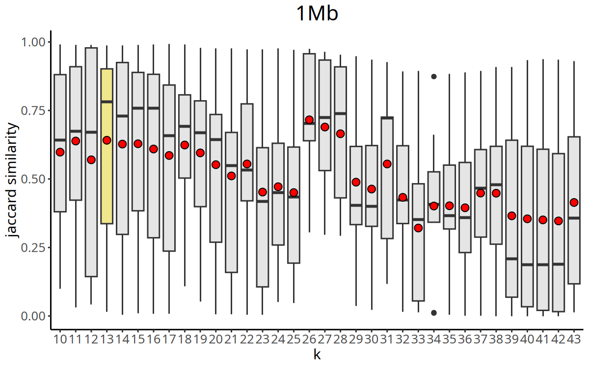
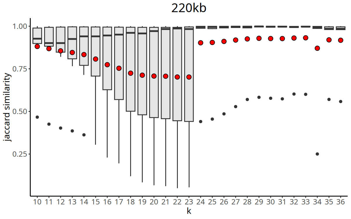
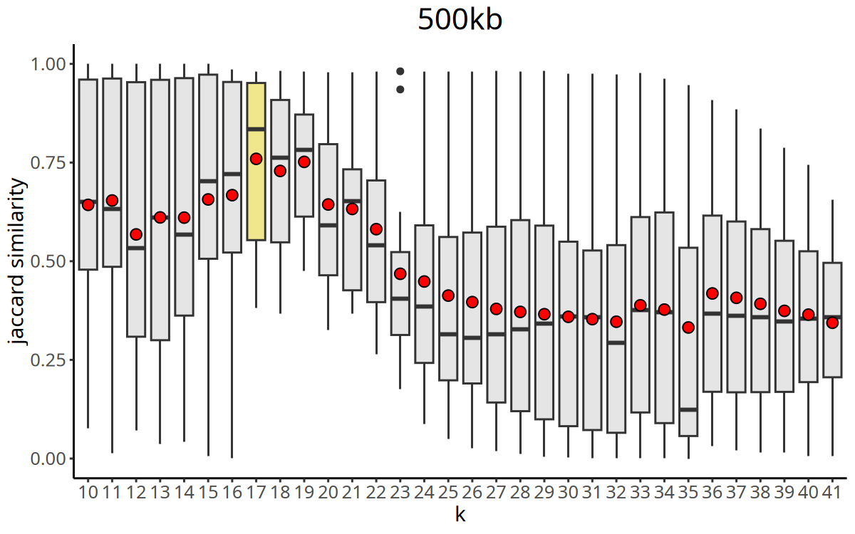
Tumor Subclonal Clustering and Clonal Evolution Analysis

Find Optimal K (findSuggestedK): Automatically recommend the most suitable number of nearest neighbors for clustering by calculating Jaccard similarity under different K values.
Perform Clustering (findClusters): Perform unsupervised clustering based on UMAP coordinates to identify different tumor subclones. Defaults to HDBSCAN algorithm. Compared to traditional Louvain/Leiden, HDBSCAN is more sensitive in identifying noise points (labeled as c0).
Build Consensus Profiles: Single-cell data inevitably contains random noise. To accurately infer tumor evolutionary history, we no longer focus on minor fluctuations of single cells, but calculate the Consensus Profile for each subclone via calcConsensus. This function takes the median of all cells in that subclone at each Bin to construct a "virtual cell" representing the clone's characteristics, greatly improving signal-to-noise ratio.
Construct Subclone Phylogenetic Tree: The runConsensusPhylo function calculates Manhattan distances between subclones based on their consensus profiles and constructs a phylogenetic tree.

About Outlier Cluster 'c0'
The HDBSCAN algorithm may classify a subset of cells into the c0 cluster. These cells typically cannot be assigned to any major clone due to:
Data Noise: Low sequencing quality leading to blurred copy number features.
Rare Clones: Cell count too low to reach the minimum threshold for independent clustering.
Doublets/Degradation: Abnormal signals caused by technical errors.
Recommendation: Before analyzing the main evolutionary structure of the tumor, it is usually recommended to remove the c0 cluster to avoid interfering with phylogenetic tree construction.

Figure Legend: Curve of Jaccard similarity index versus K value.
X-axis: K value (number of nearest neighbors).
Y-axis: Jaccard Index (clustering stability metric).
CopyKit automatically selects the K value with the maximum Jaccard similarity as the parameter for the subsequent findClusters.

options(repr.plot.width = 8, repr.plot.height = 5)
for(i in names(tumor_list)){
    suppressMessages({tumor_list[[i]] <- findSuggestedK(tumor_list[[i]])})
    pic <- plotSuggestedK(tumor_list[[i]]) + 
        ggtitle(i) + 
        theme(plot.title = element_text(hjust = .5, size = 20))
    print(pic)
    ggsave(file.path(outdir, paste0('SuggestedK_',samplename,'_',i,'.pdf')), pic, width = 8, height = 5)
}

output

|======================================================================| 100% 22 23 24 25 26 27 28 29 30 31 32 33 34 35 36 37 38 39 40 4143

for(i in names(tumor_list)){
    tumor_list[[i]] <- findClusters(tumor_list[[i]])
}

output

Using suggested k_subclones = 13

Finding clusters, using method: hdbscan

Found 495 outliers cells (group 'c0')

Found 15 subclones.

Done.

Using suggested k_subclones = 29

Finding clusters, using method: hdbscan

Found 2 outliers cells (group 'c0')

Found 5 subclones.

Done.

Using suggested k_subclones = 17

Finding clusters, using method: hdbscan

Found 438 outliers cells (group 'c0')

Found 11 subclones.

Done.

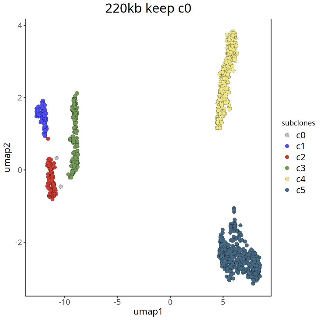
Tumor Subclonal Analysis Results at 220kb Resolution

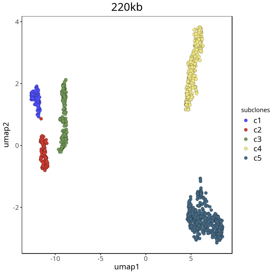
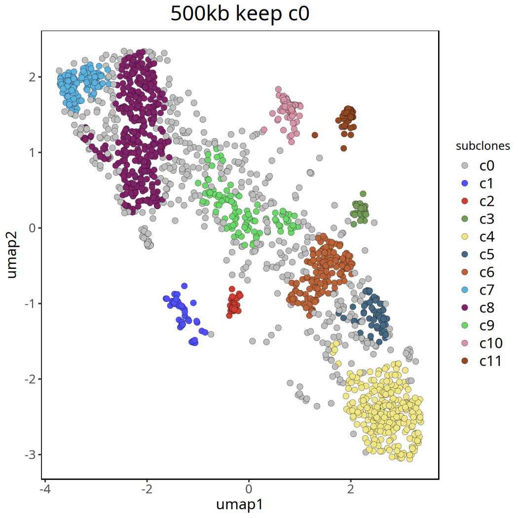
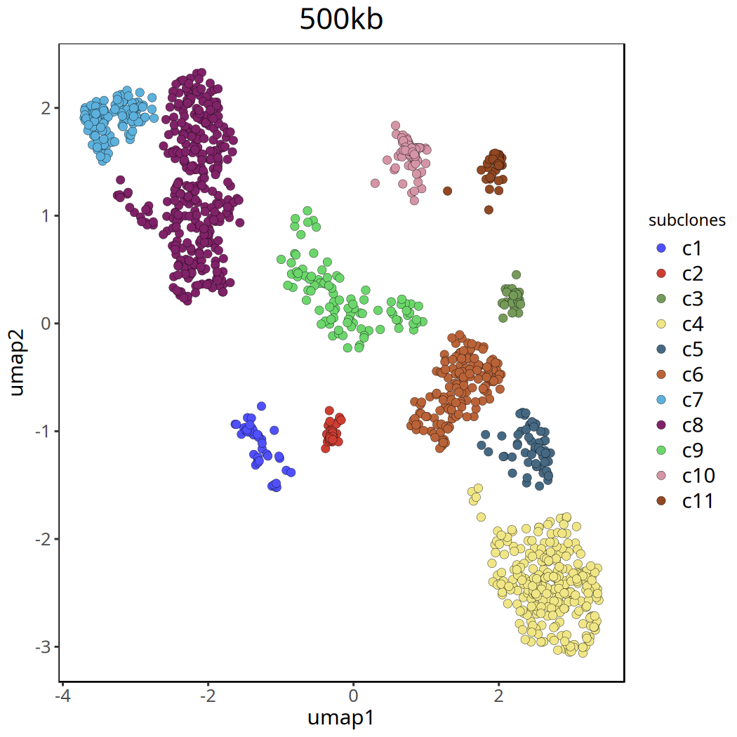
Below shows UMAP clustering plots before and after removing the c0 cluster.

Figure Legend: UMAP clustering plot after removing c0. Different colors clearly show the major subclone structure within the tumor.

options(repr.plot.width = 7, repr.plot.height = 7)
pic <- plotUmap(tumor_list[['220kb']], label = 'subclones') +
ggtitle('220kb keep c0') + 
theme(plot.title = element_text(hjust = .5, size = 20))
pic
ggsave(file.path(outdir, paste0('plotUmap',samplename,'_',i,'_keep_c0.pdf')), pic, width = 7, height = 7)

output

Plotting Umap.

Coloring by: subclones.

tumor_list[['220kb']] <- tumor_list[['220kb']][,colData(tumor_list[['220kb']])$subclones != 'c0']
pic <- plotUmap(tumor_list[['220kb']], label = 'subclones') +
ggtitle('220kb') + 
theme(plot.title = element_text(hjust = .5, size = 20))
pic
ggsave(file.path(outdir, paste0('plotUmap',samplename,'_',i,'_remove_c0.pdf')), pic, width = 7, height = 5)

output

Plotting Umap.

Coloring by: subclones.

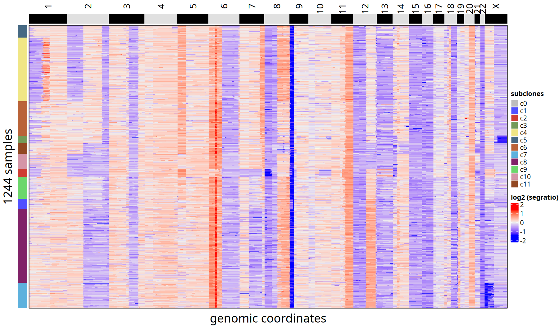
Tumor Subclone CNV Heatmap and Clonal Phylogenetic Tree at 220kb Resolution

Figure Legend: Subclone Consensus Heatmap.
Heatmap: Each row represents a cell, ordered by phylogenetic tree. Color represents Log2 Segment Ratio.
Left Annotation: Labels the subclone ID to which the cell belongs.

options(repr.plot.width = 12, repr.plot.height = 6, repr.plot.res = 150)
tumor_list[['220kb']] <- calcConsensus(tumor_list[['220kb']])
tumor_list[['220kb']] <- runConsensusPhylo(tumor_list[['220kb']])
suppressMessages({
    ht <- plotHeatmap(
      tumor_list[['220kb']],
      label = 'subclones',
      order_cells = 'consensus_tree'
    )  
})
ht 
pdf(
    file.path(outdir, paste0('plotHeatmap_consensus_tree_',samplename,'_',i,'.pdf')),  
    width = 16, 
    height = 6)
ht
dev.off()

output

|======================================================================| 100%

pdf: 2

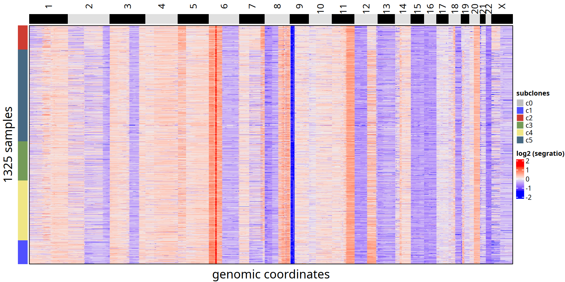
Figure Legend: Subclone Phylogenetic Tree.
Branch Length: Represents Manhattan distance, i.e., magnitude of difference in genomic CNV profiles between subclones.
Structure: Shows how the tumor evolved from the root into different branches (subclones).

suppressWarnings({
    pic <- plotPhylo(tumor_list[['220kb']], label = 'subclones', consensus = TRUE)
})
pic
ggsave(file.path(outdir, paste0('plotPhylo_consensus_',samplename,'_220kb','.pdf')), pic, width = 7, height = 5)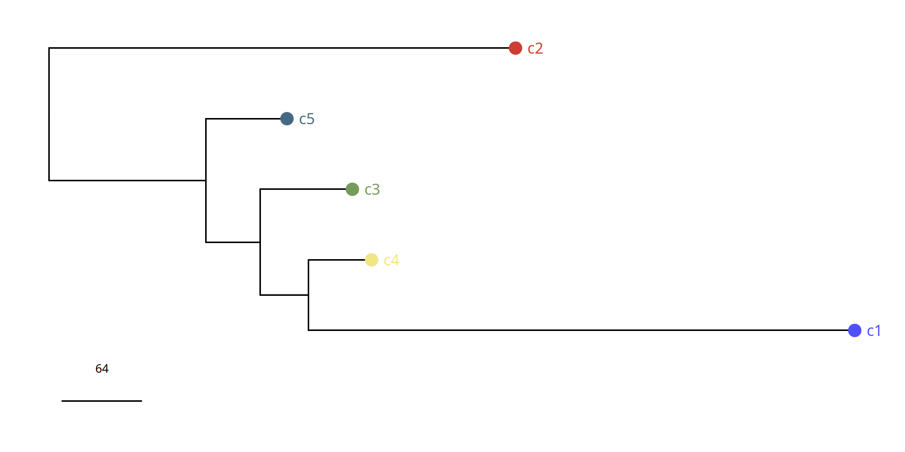

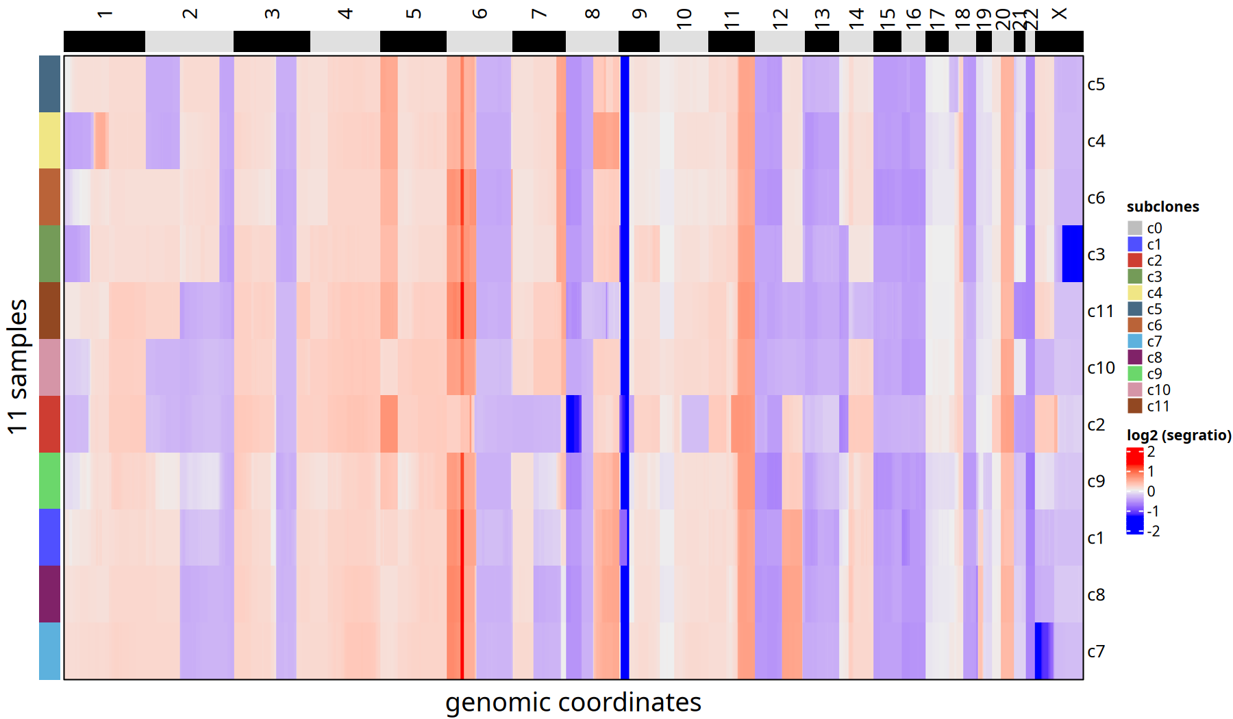
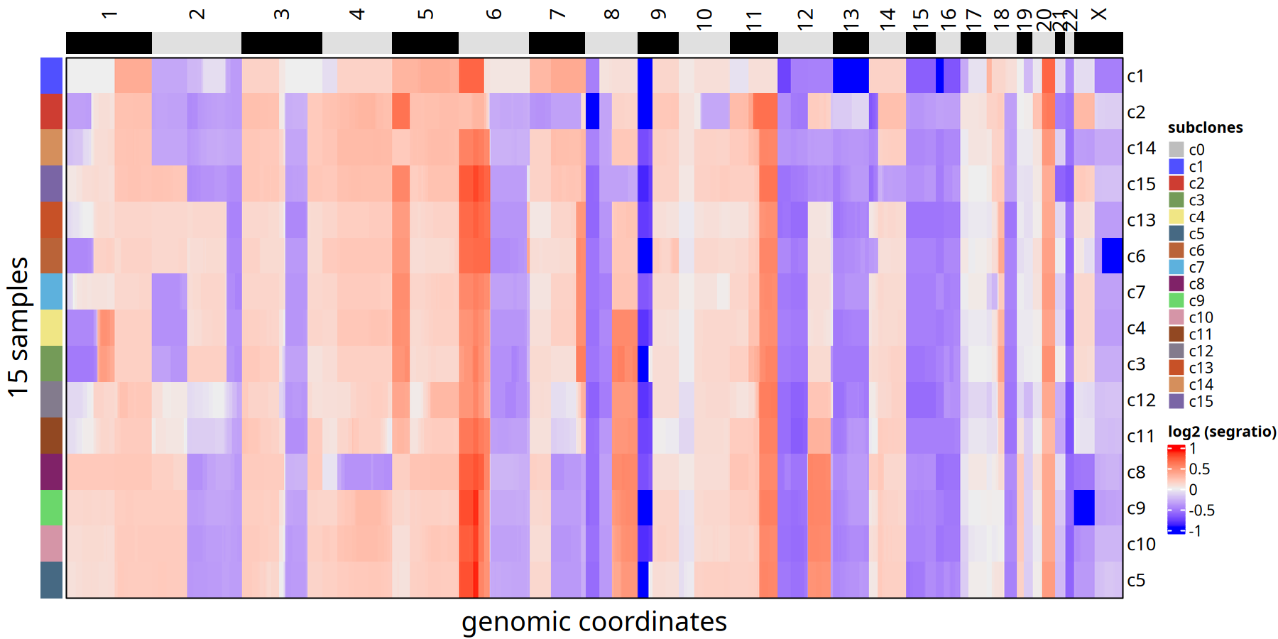
The heatmap and line plot below show CNV differences between subclones at the "Bulk" level (i.e., subclone consensus level).

Figure Legend: Subclone Consensus Heatmap.
Unlike the single-cell heatmap, here each row represents only one subclone (not a single cell). This eliminates single-cell noise and clearly displays core CNV events of each subclone (e.g., whole chromosome arm amplification or deletion).

tumor_list[['220kb']]  <- calcConsensus(tumor_list[['220kb']] )
suppressMessages({
    ht <- plotHeatmap(tumor_list[['220kb']],consensus = TRUE,label = 'subclones')
})
ht
pdf(
    file.path(outdir, paste0('plotHeatmap_consensus_tree_',samplename,'_220kb','.pdf')),  
    width = 16, 
    height = 6)
ht
dev.off()

output

|======================================================================| 100%

pdf: 2

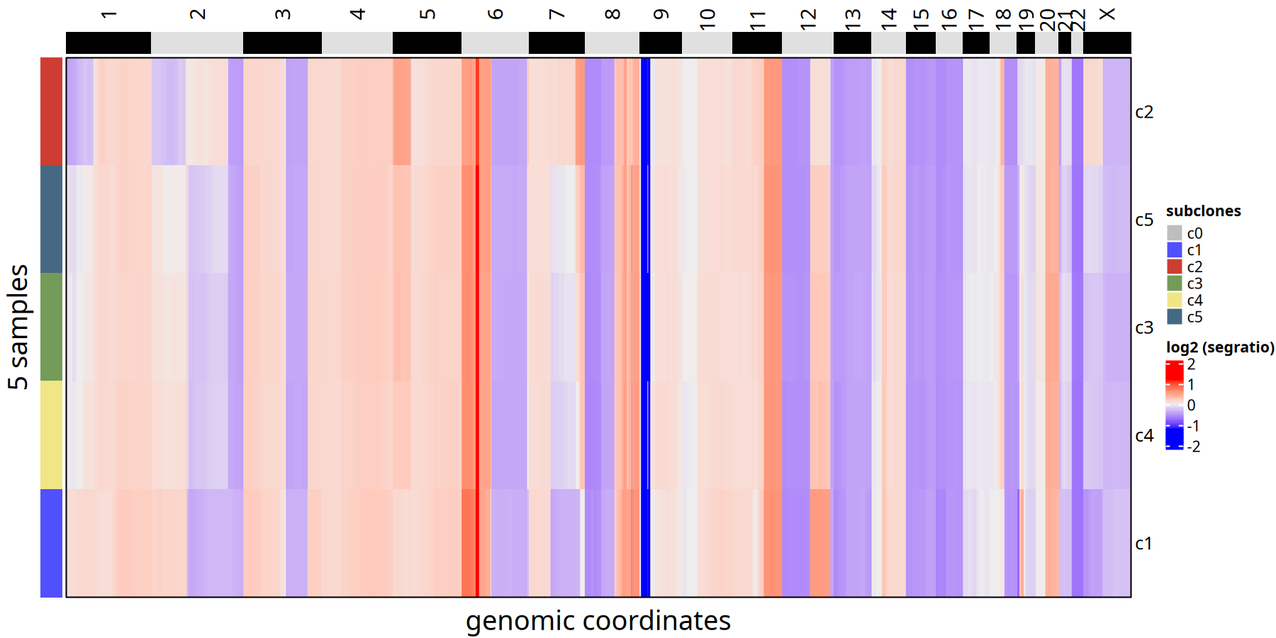
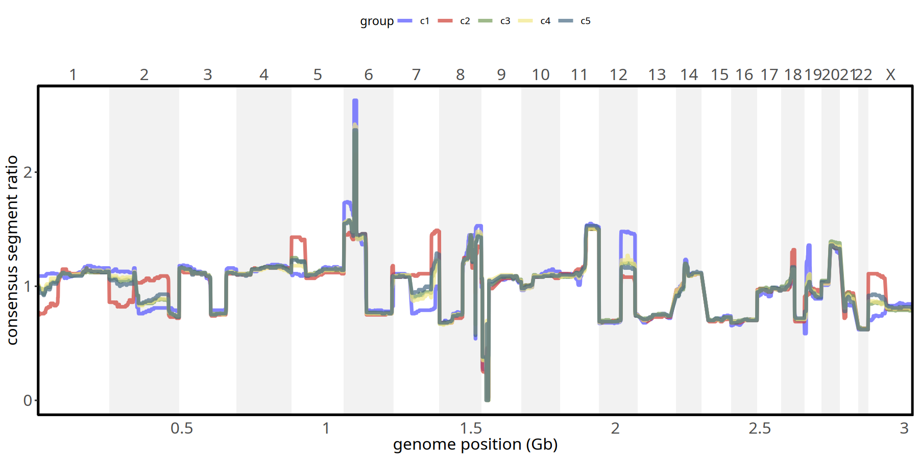
Figure Legend: Subclone Copy Number Profile.
X-axis: Genomic chromosome position (chr1 - chr22).
Y-axis: Consensus Segment Ratio (median value of each segment within the subclone).
Meaning: Different colored lines represent different subclones. Bulges above baseline (1.0) indicate amplification, depressions indicate deletion. Allows precise comparison of differences between subclones at specific loci.

pic <- plotConsensusLine_static(tumor_list[['220kb']],levels(colData(tumor_list[['220kb']])$subclones) ) +
scale_color_manual(values = subclones_pal())
pic
ggsave(file.path(outdir, paste0('plot_ConsensusLine_',samplename,'_220kb','.pdf')), pic, width = 7, height = 5)

output

Warning message:
“The \`size\` argument of \`element_rect()\` is deprecated as of ggplot2 3.4.0.
ℹ Please use the \`linewidth\` argument instead.”
Warning message:
“Using \`size\` aesthetic for lines was deprecated in ggplot2 3.4.0.
ℹ Please use \`linewidth\` instead.”

Tumor Subclone Analysis Results at 500kb Resolution

Below shows UMAP clustering plots before and after removing the c0 cluster.

options(repr.plot.width = 7, repr.plot.height = 7)
pic <- plotUmap(tumor_list[['500kb']], label = 'subclones') +
ggtitle('500kb keep c0') + 
theme(plot.title = ggplot2::element_text(hjust = .5, size = 20))

pic
ggsave(file.path(outdir, paste0('plotUmap',samplename,'_1Mb','_keep_c0.pdf')), pic, width = 7, height = 5)

output

Plotting Umap.

Coloring by: subclones.

tumor_list[['500kb']] <- tumor_list[['500kb']][,colData(tumor_list[['500kb']])$subclones != 'c0']
pic <- plotUmap(tumor_list[['500kb']], label = 'subclones') +
ggtitle('500kb') + 
theme(plot.title = element_text(hjust = .5, size = 20))
pic
ggsave(file.path(outdir, paste0('plotUmap',samplename,'_500kb','_remove_c0.pdf')), pic, width = 7, height = 5)

output

Plotting Umap.

Coloring by: subclones.

Tumor Subclone CNV Heatmap and Clonal Phylogenetic Tree at 500kb Resolution

options(repr.plot.width = 12, repr.plot.height = 7, repr.plot.res = 150)
tumor_list[['500kb']] <- calcConsensus(tumor_list[['500kb']])
tumor_list[['500kb']] <- runConsensusPhylo(tumor_list[['500kb']])
suppressMessages({
ht <- plotHeatmap(
  tumor_list[['500kb']],
  label = 'subclones',
  order_cells = 'consensus_tree'
)})
ht
pdf(
    file.path(outdir, paste0('plotHeatmap_consensus_tree_',samplename,'_550kb','.pdf')),  
    width = 16, 
    height = 6)
ht
dev.off()

output

|======================================================================| 100%

pdf: 2

suppressWarnings({
    pic <- plotPhylo(tumor_list[['500kb']], label = 'subclones', consensus = TRUE)
})
pic
ggsave(file.path(outdir, paste0('plotPhylo_consensus_',samplename,'_500kb','.pdf')), pic, width = 7, height = 7)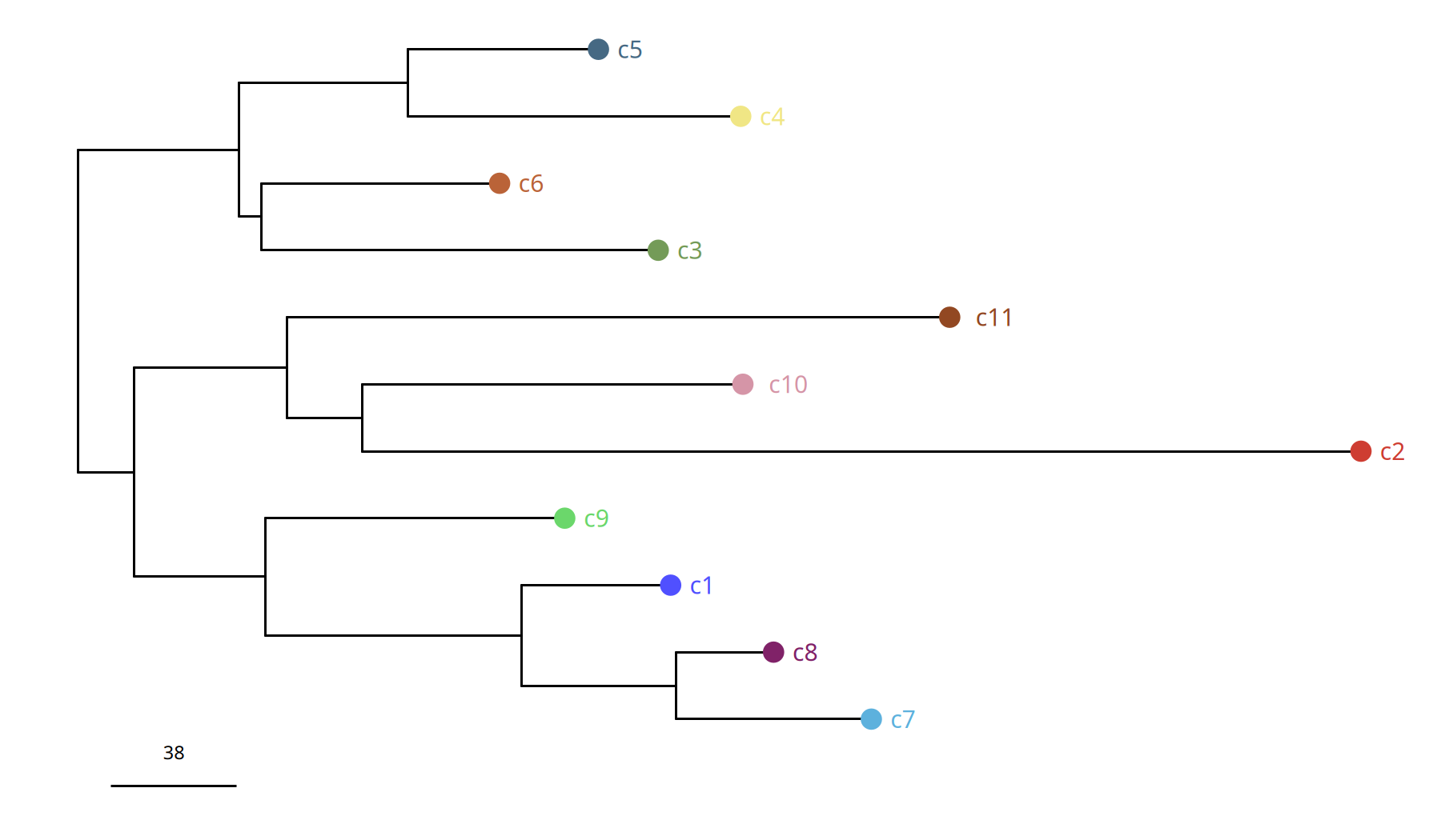

The heatmap and line plot below show CNV differences between subclones at the "Bulk" level.

tumor_list[['500kb']]  <- calcConsensus(tumor_list[['500kb']] )
suppressMessages({
    ht <- plotHeatmap(tumor_list[['500kb']],consensus = TRUE,label = 'subclones')
})
ht
pdf(
    file.path(outdir, paste0('plotHeatmap_consensus_',samplename,'_550kb','.pdf')),  
    width = 16, 
    height = 6)
ht
dev.off()

output

|======================================================================| 100%

pdf: 2

pic <- plotConsensusLine_static(tumor_list[['500kb']],levels(colData(tumor_list[['500kb']])$subclones) ) +
scale_color_manual(values = subclones_pal())
pic
ggsave(file.path(outdir, paste0('plot_ConsensusLine_',samplename,'_500kb','.pdf')), pic, width = 7, height = 5)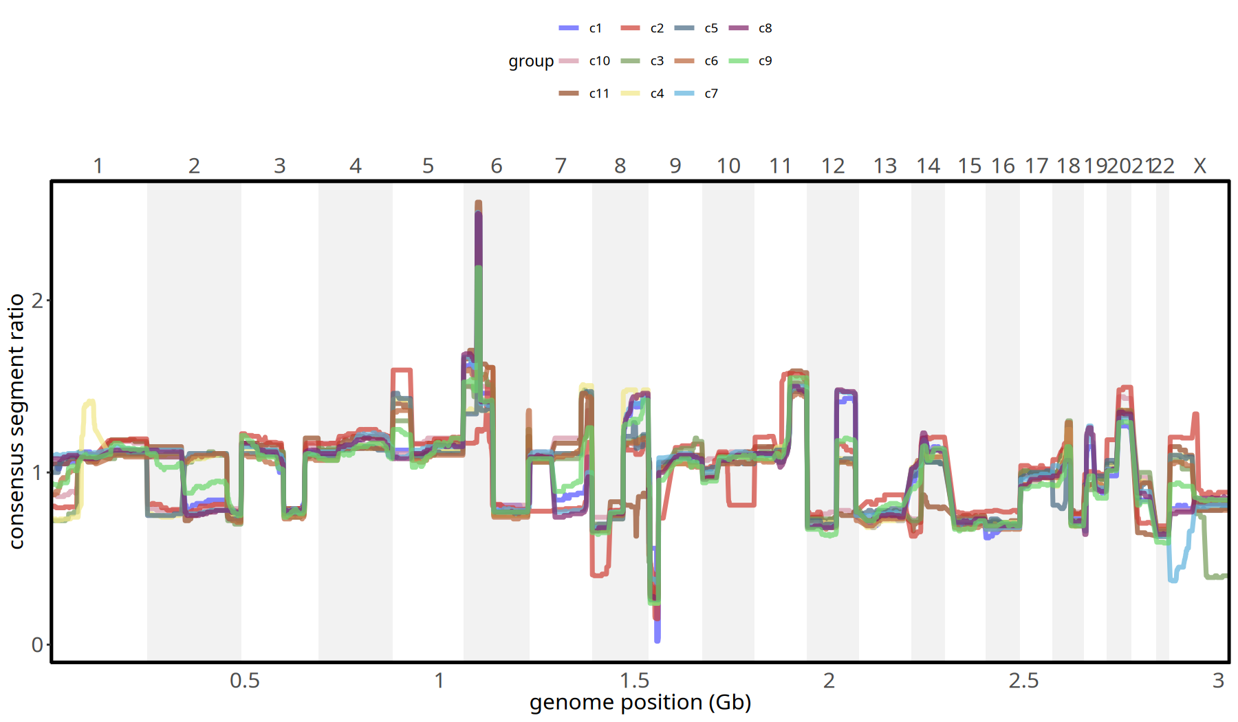

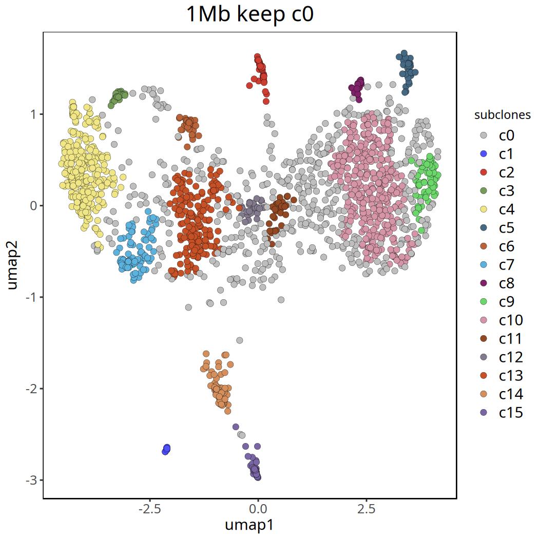
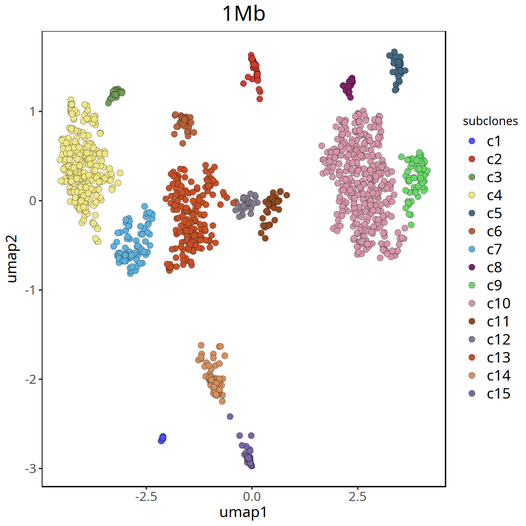
Tumor Subclonal Analysis Results at 1Mb Resolution

Below shows UMAP clustering plots before and after removing the c0 cluster.

options(repr.plot.width = 7, repr.plot.height = 7)
pic <- plotUmap(tumor_list[['1Mb']], label = 'subclones') +
ggtitle('1Mb keep c0') + 
theme(plot.title = element_text(hjust = .5, size = 20))
pic
ggsave(file.path(outdir, paste0('plotUmap_',samplename,'1Mb','_keep_c0.pdf')), pic, width = 7, height = 5)

output

Plotting Umap.

Coloring by: subclones.

options(repr.plot.width = 7, repr.plot.height = 7)
tumor_list[['1Mb']] <- tumor_list[['1Mb']][,colData(tumor_list[['1Mb']])$subclones != 'c0']
pic <- plotUmap(tumor_list[['1Mb']], label = 'subclones') +
ggtitle('1Mb') + 
theme(plot.title = element_text(hjust = .5, size = 20))
pic
ggsave(file.path(outdir, paste0('plotUmap_',samplename,'_1Mb','_remove_c0.pdf')), pic, width = 7, height = 5)

output

Plotting Umap.

Coloring by: subclones.

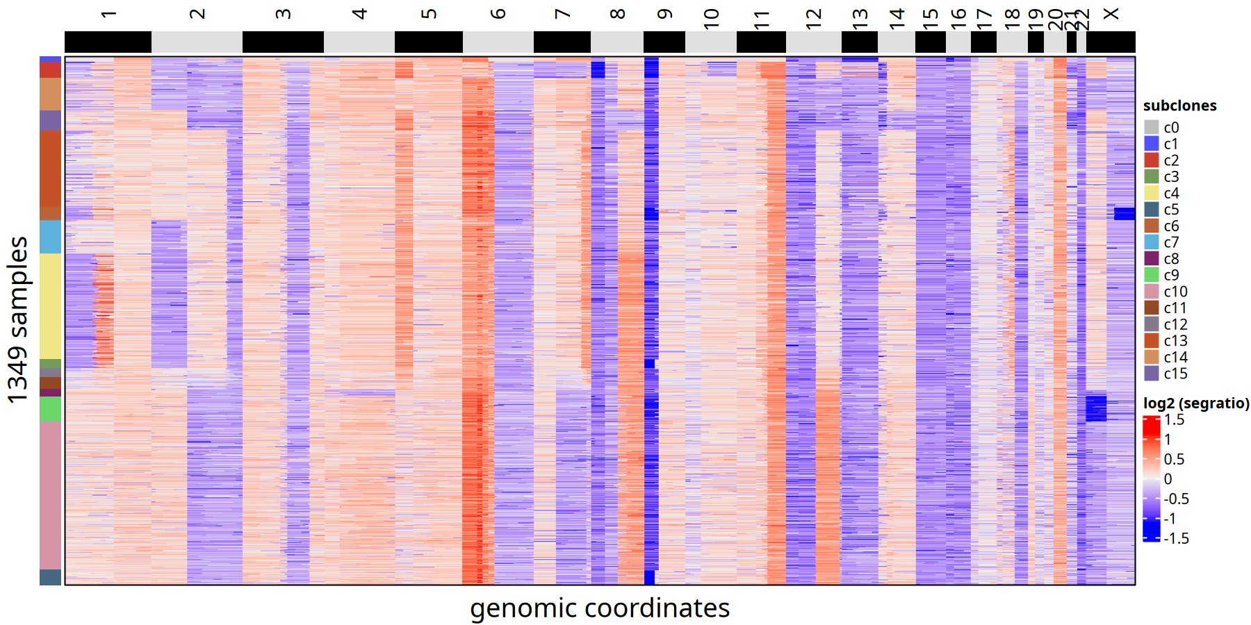
Tumor Subclone CNV Heatmap and Clonal Phylogenetic Tree at 1Mb Resolution

options(repr.plot.width = 12, repr.plot.height = 6, repr.plot.res = 150)
tumor_list[['1Mb']] <- calcConsensus(tumor_list[['1Mb']])
tumor_list[['1Mb']] <- runConsensusPhylo(tumor_list[['1Mb']])
suppressMessages({
    ht <- plotHeatmap(
      tumor_list[['1Mb']],
      label = 'subclones',
      order_cells = 'consensus_tree'
    )
})
ht
pdf(
    file.path(outdir, paste0('plotHeatmap_consensus_tree_',samplename,'_1Mb','.pdf')),  
    width = 16, 
    height = 6)
ht
dev.off()

output

|======================================================================| 100%

pdf: 2

suppressWarnings({
    pic <- plotPhylo(tumor_list[['1Mb']], label = 'subclones', consensus = TRUE)
})
pic
ggsave(file.path(outdir, paste0('plotPhylo_consensus_',samplename,'_1Mb','.pdf')), pic, width = 7, height = 7)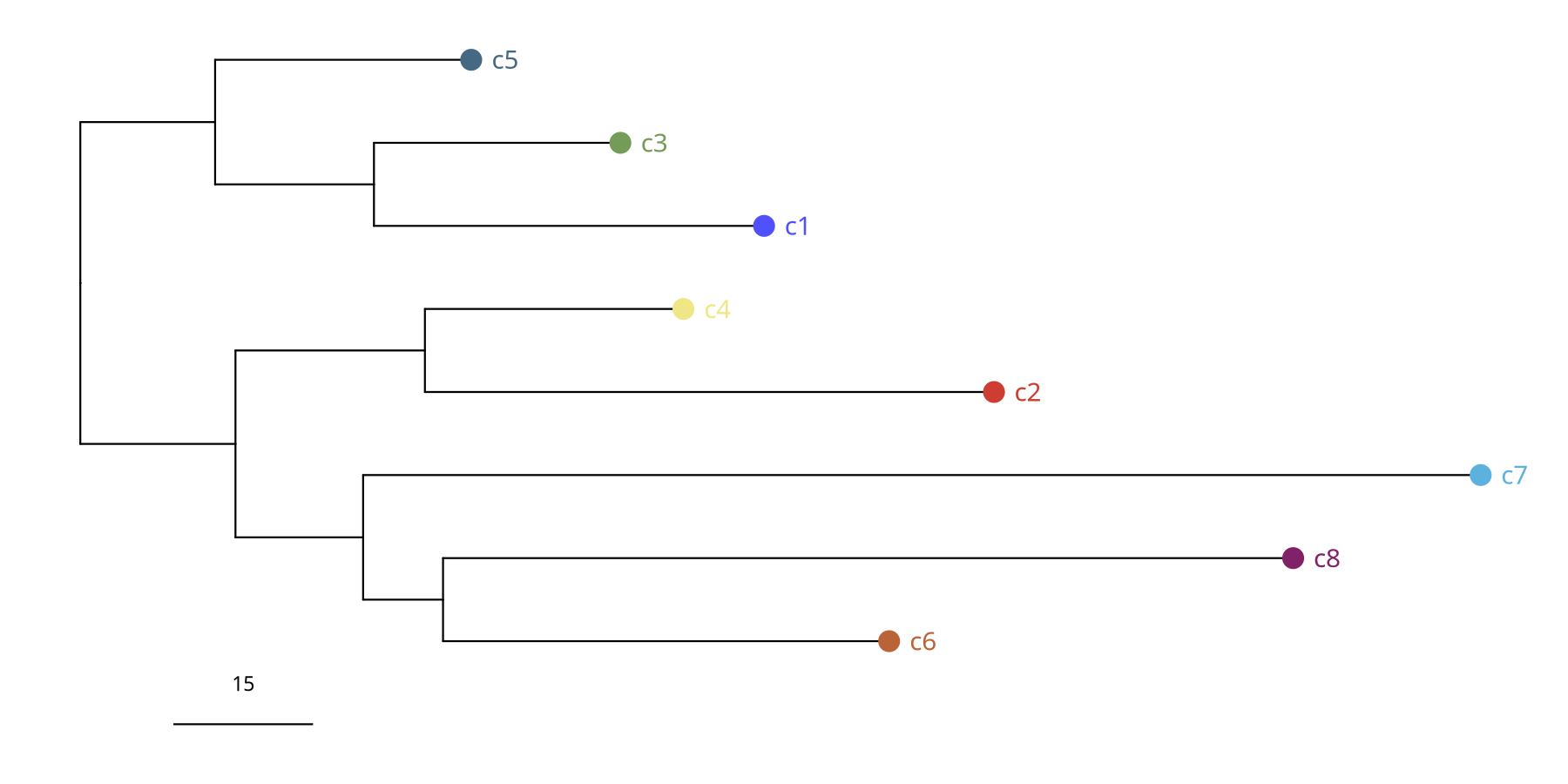

The heatmap and line plot below show CNV differences between subclones at the "Bulk" level.

suppressMessages({
    ht <- plotHeatmap(tumor_list[['1Mb']],consensus = TRUE,label = 'subclones')
})
ht
pdf(
    file.path(outdir, paste0('plotHeatmap_consensus_',samplename,'_550kb','.pdf')),  
    width = 16, 
    height = 6)
ht
dev.off()

pdf: 2

pic <- plotConsensusLine_static(tumor_list[['1Mb']],levels(colData(tumor_list[['1Mb']])$subclones) ) +
scale_color_manual(values = subclones_pal())
pic
ggsave(file.path(outdir, paste0('plot_ConsensusLine_',samplename,'_1Mb','.pdf')), pic, width = 7, height = 5)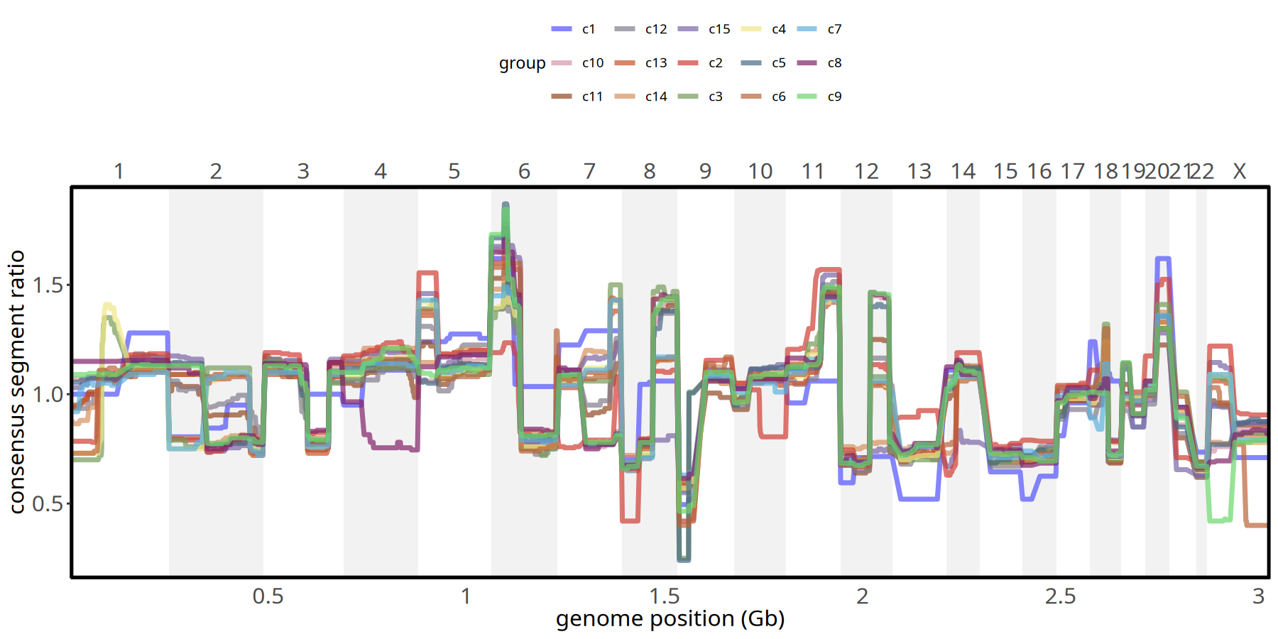

Single-cell Level Phylogenetic Tree

In addition to subclone-level evolutionary trees, CopyKit can construct single-cell resolution evolutionary trees via runPhylo. This helps observe micro-evolution processes within clones.

Principle: Calculates distance between cells based on copy number profile similarity. The more similar the copy numbers, the closer the relationship.
Note: Computation is intensive due to the massive amount of single-cell data and high noise levels.

220kb Resolution Single Cell Phylogenetic Tree

Figure Legend: Single-cell Resolution Phylogenetic Tree.
Terminal Nodes: Each point in the tree represents an individual cell.
Color: Identifies the subclone to which the cell belongs.
Significance: Compared to the subclone tree, this plot reveals internal subclone structure, useful for observing subtle heterogeneity between cells.

suppressMessages({
    tumor_list[['220kb']] <- runPhylo(tumor_list[['220kb']], metric = 'manhattan')
    pic <- plotPhylo(tumor_list[['220kb']], label = 'subclones')
})

pic
ggsave(file.path(outdir, paste0('plotPhylo_cells_',samplename,'_220kb.pdf')), width = 8, height = 6)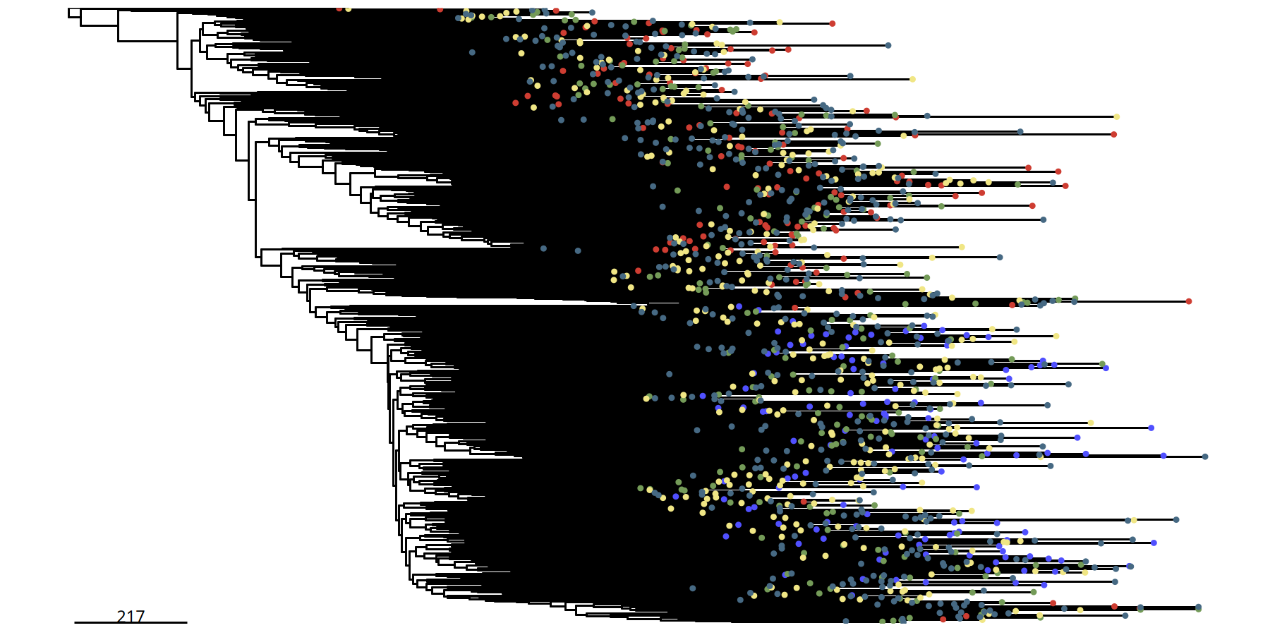

500kb Resolution Single Cell Phylogenetic Tree

suppressMessages({
    tumor_list[['500kb']] <- runPhylo(tumor_list[['500kb']], metric = 'manhattan')
    pic <- plotPhylo(tumor_list[['500kb']], label = 'subclones')
})

pic
ggsave(file.path(outdir, paste0('plotPhylo_cells_',samplename,'_500kb.pdf')), width = 8, height = 6)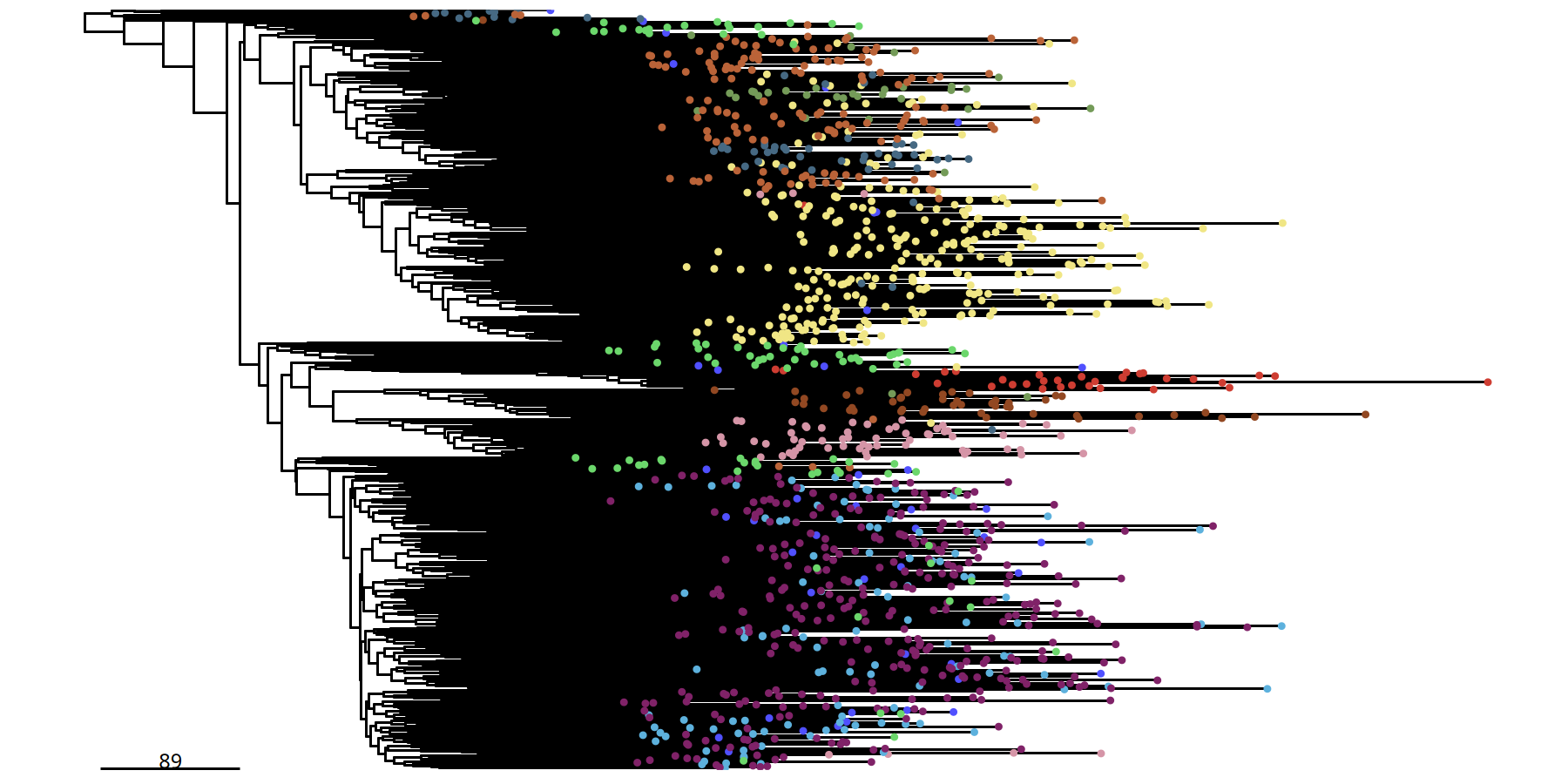

Single-cell Phylogenetic Tree at 1Mb Resolution

suppressMessages({
    tumor_list[['1Mb']] <- runPhylo(tumor_list[['1Mb']], metric = 'manhattan')
    pic <- plotPhylo(tumor_list[['1Mb']], label = 'subclones')
})

pic
ggsave(file.path(outdir, paste0('plotPhylo_cells_',samplename,'_1Mb.pdf')), width = 8, height = 6)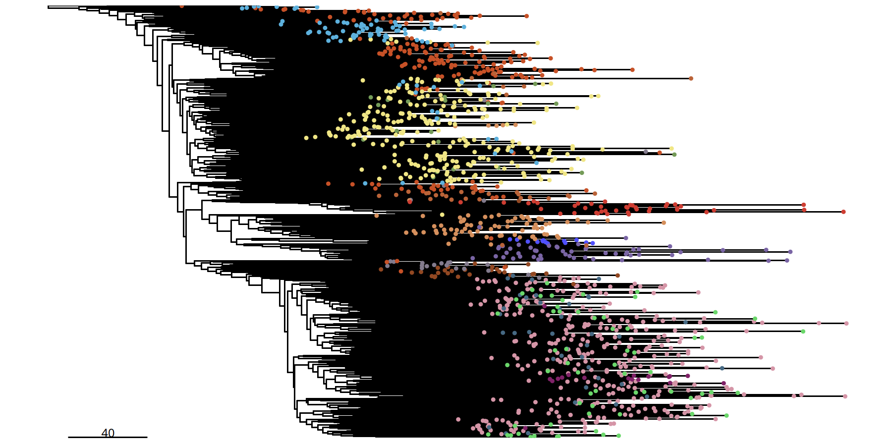

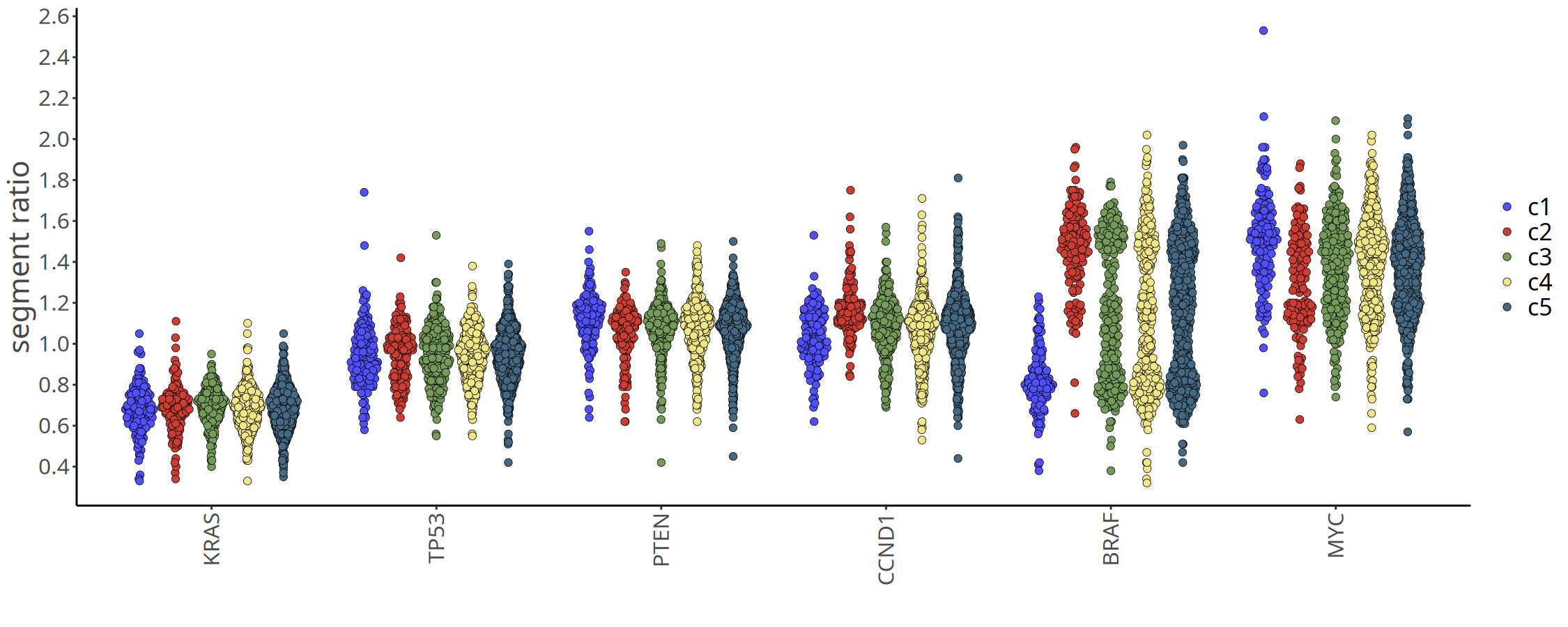
Gene-level CNV Visualization

Besides genome-wide profiles, we usually focus on copy number status of specific driver genes (e.g., MYC, TP53, EGFR). The plotGeneCopy function displays copy number distribution of specific genes across subclones. The figure below shows dot plots of driver gene copy numbers only for subclones identified at 220kb resolution.

Tip: You can replace the genes in the list with target genes of interest. Note: If certain genes are located in exclusion regions of the VarBin algorithm (e.g., centromeres, telomeres, or highly repetitive regions), they cannot be detected (warning messages will be displayed).

Figure Legend: Driver Gene Copy Number Jitter Plot.
X-axis: Different tumor subclones.
Y-axis: Inferred absolute Integer Copy Number.
Meaning: Each dot represents a cell. Intuitively displays amplification or deletion status of key oncogenes (e.g., MYC, EGFR) or tumor suppressor genes (e.g., TP53, PTEN) in different subclones, helping identify key variation events driving tumor evolution.

options(repr.plot.height = 6, repr.plot.width = 15)
suppressMessages({
    plotGeneCopy(
        tumor_list[['220kb']], 
        genes = c("TP53","PTEN","MYC","CCND1","KRAS","BRAF"),
        label = 'subclones',
        dodge.width = 0.8)
})

saveRDS(tumor_list, file.path(outdir, paste0(samplename, '_copykit_analysis.rds')))

More Features: For more advanced visualization features of CopyKit, please see the CopyKit Official Documentation.

scMethyl + RNA Multi-omics: CNV Copy Number Variation Analysis (Based on CopyKit) ​

Module Introduction ​

Input File Preparation ​

Option A: Import Analyzed Results Directly (Recommended) ​

Option B: Start from Single-cell BAM Files ​

CopyKit Analysis Pipeline ​

Key Parameter Settings ​

Best Practice Recommendations ​

Data Preprocessing Principle ​

Quality Control ​

Key QC Metrics ​

Normal Diploid Cell Filtering ​

CNV results for diploid and aneuploid at 220kb bin ​

CNV Results for Diploid and Aneuploid at 500kb bin ​

CNV results for diploid and aneuploid at 1Mb bin ​

Outlier Cell Filtering ​

CNV Heatmap Comparison between Outliers and Retained Cells at 220kb Resolution ​

CNV Heatmap Comparison of Outlier vs Retained Cells at 500kb Resolution ​

CNV Heatmap Comparison between Outliers and Retained Cells at 1Mb Resolution ​

KNN Smoothing ​

Clustering Analysis and Subclonal Evolution Analysis ​

Dimensionality Reduction ​

Absolute Ploidy Inference ​

Tumor Subclonal Clustering and Clonal Evolution Analysis ​

Tumor Subclonal Analysis Results at 220kb Resolution ​

Tumor Subclone Analysis Results at 500kb Resolution ​

Tumor Subclonal Analysis Results at 1Mb Resolution ​

Single-cell Level Phylogenetic Tree ​

220kb Resolution Single Cell Phylogenetic Tree ​

500kb Resolution Single Cell Phylogenetic Tree ​

Single-cell Phylogenetic Tree at 1Mb Resolution ​

Gene-level CNV Visualization ​

scMethyl + RNA Multi-omics: CNV Copy Number Variation Analysis (Based on CopyKit)

Module Introduction

Input File Preparation

Option A: Import Analyzed Results Directly (Recommended)

Option B: Start from Single-cell BAM Files

CopyKit Analysis Pipeline

Key Parameter Settings

Best Practice Recommendations

Data Preprocessing Principle

Quality Control

Key QC Metrics

Normal Diploid Cell Filtering

CNV results for diploid and aneuploid at 220kb bin

CNV Results for Diploid and Aneuploid at 500kb bin

CNV results for diploid and aneuploid at 1Mb bin

Outlier Cell Filtering

CNV Heatmap Comparison between Outliers and Retained Cells at 220kb Resolution

CNV Heatmap Comparison of Outlier vs Retained Cells at 500kb Resolution

CNV Heatmap Comparison between Outliers and Retained Cells at 1Mb Resolution

KNN Smoothing

Clustering Analysis and Subclonal Evolution Analysis

Dimensionality Reduction

Absolute Ploidy Inference

Tumor Subclonal Clustering and Clonal Evolution Analysis

Tumor Subclonal Analysis Results at 220kb Resolution

Tumor Subclone Analysis Results at 500kb Resolution

Tumor Subclonal Analysis Results at 1Mb Resolution

Single-cell Level Phylogenetic Tree

220kb Resolution Single Cell Phylogenetic Tree

500kb Resolution Single Cell Phylogenetic Tree

Single-cell Phylogenetic Tree at 1Mb Resolution

Gene-level CNV Visualization