scMethyl + RNA Multi-omics: Doublet Detection Workflow

Author: SeekGene

Time: 28 min

Words: 5.4k words

Updated: 2026-02-28

Reads: 0 times

scMethyl + RNA-seq Analysis Guide Notebooks

Module Introduction

This module is based on ALLCools and MethylScrublet algorithms, designed to identify and filter doublets from single-cell methylation sequencing data.

Doublets refer to technical artifacts where two or more cells accidentally stick together and are sequenced as a single "cell" during single-cell sequencing. Doublets introduce mixed expression/methylation signatures, seriously interfering with subsequent cell clustering and differential analysis (e.g., potentially misidentifying doublets as new intermediate cell types).

This module provides three complementary doublet identification methods, which can be combined to judge and improve identification accuracy:

• Method 1: Transcriptome Cell Type Identification: Identifies doublets based on RNA-seq data by detecting abnormal co-expression of marker genes from different cell types.
• Method 2: Methylation Reads Count Identification: Identifies potential doublets with abnormally high coverage by analyzing the methylation sequencing depth (Reads count) distribution of each cell.
• Method 3: Methylation Rate Identification (MethylScrublet): Uses MethylScrublet algorithm to calculate a "doublet score" for each cell by simulating artificial doublets and comparing with observed data.

TIP

This analysis applies to Single-cell Multi-omics Data (containing both RNA and methylation info), and also supports doublet identification using only methylation data.

Input File Preparation

This module requires the following input files:

Required Files

• Single-cell RNA-seq Data: Gene expression matrix (filtered_feature_bc_matrix directory).
• Single-cell Methylation Data: Methylation dataset in MCDS format (.mcds file).
• Barcode Mapping File (Optional): If the reagent type is DD-MET3, used to associate cell Barcodes between RNA and methylation data.

File Structure Example

data/
├── AY1768874914782
│   └── methylation
│       └── demoWTJW969-task-1
│           └── WTJW969
│               ├── allcools_generate_datasets
│               │   └── WTJW969.mcds # Methylation Data
│               ├── filtered_feature_bc_matrix # Transcriptome Expression Matrix
│               └── split_bams
│                   ├── WTJW969_cells.csv
│                   └── filtered_barcode_reads_counts.csv
└── AY1768876253533
    └── methylation
        └── demo4WTJW880-task-1
            └── WTJW880
                ├── allcools_generate_datasets
                                │   └── WTJW880.mcds # Methylation data
                                ├── filtered_feature_bc_matrix # Transcriptome expression matrix
                └── split_bams
                    ├── WTJW880_cells.csv
                    └── filtered_barcode_reads_counts.csv

DD-M_bUCB3_whitelist.csv  # Barcode mapping file (optional)

# --- Import necessary Python packages ---

# System operations and file handling
import os
import re
import glob
import warnings

# ALLCools related packages: for methylation data processing and doublet detection
from ALLCools.mcds import MCDS
from ALLCools.clustering import (
    tsne, significant_pc_test, log_scale, lsi, 
    binarize_matrix, filter_regions, cluster_enriched_features, 
    ConsensusClustering, Dendrogram, get_pc_centers
)
from ALLCools.clustering.doublets import MethylScrublet
from ALLCools.plot import *

# Single-cell Analysis Tools
import scanpy as sc

# Data Processing and Visualization
import numpy as np
import pandas as pd
import matplotlib.pyplot as plt
import matplotlib.colors as mcolors
from matplotlib.lines import Line2D
import seaborn as sns
from matplotlib.patches import Rectangle

# Other Tools
from scipy import sparse

# --- File path configuration ---
# Configure paths based on the new file hierarchy
# Format: {Sample Name: {'top_dir': Top Directory, 'demo_dir': Demo Directory}}
sample_path_config = {
    "WTJW969": {"top_dir": "AY1768874914782", "demo_dir": "demoWTJW969-task-1"},
    "WTJW880": {"top_dir": "AY1768876253533", "demo_dir": "demo4WTJW880-task-1"}
}

# Data root directory (default is "data")
data_root = "data"

# Current sample name for analysis (can be modified as needed)
current_sample = "WTJW969"

## reagent_type: Kit type ('DD-MET3' or 'DD-MET5')
## DD-MET3: RNA and methylation data use different Barcodes, need association via mapping file
## DD-MET5: RNA and methylation data use same Barcode, no mapping file needed
reagent_type = "DD-MET5"

Doublet Identification Methods

This module provides three complementary doublet identification methods; comprehensive use is recommended to improve identification accuracy.

Method 1: Doublet Identification Based on Transcriptome Cell Type Identification

Principle Explanation:

In scRNA-seq data analysis, a common strategy for doublet identification is detecting abnormal co-expression of marker genes from different cell types.

Judgment Logic:

When two marker genes theoretically expressed in different cell types are highly expressed simultaneously in the same cell population, it suggests the population may not derive from a single cell type but is a doublet composed of two different cell types (i.e., two cells identified as one during library prep or sequencing).

Example Illustration:

For example, when T cell marker genes (e.g., CD3D) and B cell marker genes (e.g., CD79A) are highly expressed simultaneously in the same cell population, this population likely represents doublets composed of T cells and B cells.

RNA Transcriptome Data Preprocessing and Dimensionality Reduction Clustering

warnings.filterwarnings('ignore')
# --- RNA transcriptome data preprocessing and dimensionality reduction clustering ---
# Build path based on new file hierarchy: data/{top_dir}/methylation/{demo_dir}/{sample}/filtered_feature_bc_matrix
top_dir = sample_path_config[current_sample]['top_dir']
demo_dir = sample_path_config[current_sample]['demo_dir']
rna_path = os.path.join('../../',data_root, top_dir, 'methylation', demo_dir, current_sample, 'filtered_feature_bc_matrix')
adata_rna = sc.read_10x_mtx(rna_path)

# Calculate mitochondrial gene markers (for quality control)
adata_rna.var["mt"] = adata_rna.var_names.str.startswith("MT-")
sc.pp.calculate_qc_metrics(adata_rna, qc_vars=["mt"], percent_top=None, log1p=False, inplace=True)

# Data Normalization: Normalize total counts per cell to 10,000
sc.pp.normalize_total(adata_rna, target_sum=1e4)

# Log Transformation: log(x + 1) transform to make data closer to normal distribution
sc.pp.log1p(adata_rna)

# Identify highly variable genes: Select top 2000 genes with largest expression variation for subsequent analysis
sc.pp.highly_variable_genes(adata_rna, n_bins=100, n_top_genes=2000)

# Save raw data to adata.raw, then keep only highly variable genes
adata_rna.raw = adata_rna
adata_rna = adata_rna[:, adata_rna.var.highly_variable]

# Normalization: Z-score normalization, capped at 10
sc.pp.scale(adata_rna, max_value=10)

# Principal Component Analysis (PCA) Dimensionality Reduction
sc.tl.pca(adata_rna)

# Build KNN Graph (for UMAP and clustering)
sc.pp.neighbors(adata_rna)

# UMAP Dimensionality Reduction Visualization
sc.tl.umap(adata_rna)

# Leiden Clustering (Resolution 0.8)
sc.tl.leiden(adata_rna, resolution=0.8)

# Visualize UMAP results, colored by cluster
sc.set_figure_params(scanpy=True, fontsize=12, facecolor='white', figsize=(6, 6))
sc.pl.umap(adata_rna, color='leiden', s=35, palette='Set2', frameon=True)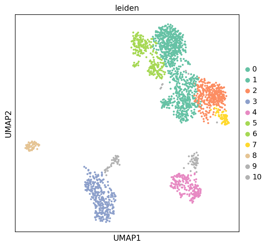

Methylome Data Preprocessing and Dimensionality Reduction Clustering

# --- Methylome data preprocessing and dimensionality reduction clustering ---
# Build path based on new file hierarchy: data/{top_dir}/methylation/{demo_dir}/{sample}/allcools_generate_datasets/{sample}.mcds
top_dir = sample_path_config[current_sample]['top_dir']
demo_dir = sample_path_config[current_sample]['demo_dir']
mcds_path = os.path.join('../../',data_root, top_dir, 'methylation', demo_dir, current_sample, 'allcools_generate_datasets', f'{current_sample}.mcds')
mcds = MCDS.open(
    mcds_path,
    obs_dim="cell",
    var_dim="chrom20k"
)

# Extract methylation score matrix (using hypo-score, i.e., hypomethylation score)
adata_methy = mcds.get_score_adata(mc_type="CGN", quant_type="hypo-score")

# Binarize matrix: Mark regions with methylation rate > 0.95 as hypermethylated
binarize_matrix(adata_methy, cutoff=0.95)

# Filter low-quality regions: Remove regions with low variability or insufficient coverage
filter_regions(adata_methy)

# LSI (Latent Semantic Indexing) Dimensionality Reduction: Similar to PCA, suitable for sparse matrices
lsi(adata_methy, algorithm="arpack", obsm="X_lsi")

# Significant Principal Component Test: Keep only significant components with p < 0.1
significant_pc_test(adata_methy, p_cutoff=0.1, obsm="X_lsi", update=True)

# Build KNN Graph (using LSI dimensionality reduction results, 30 neighbors)
sc.pp.neighbors(adata_methy, use_rep='X_lsi', n_neighbors=30)

# UMAP Dimensionality Reduction Visualization
sc.tl.umap(adata_methy)

# Leiden Clustering (Resolution 0.5)
sc.tl.leiden(adata_methy, resolution=0.5)

output

Loading chunk 0-2196/2196
126195 regions remained.
16 components passed P cutoff of 0.1.
Changing adata.obsm['X_pca'] from shape (2196, 100) to (2196, 16)

Cell Type Marker Gene Expression Analysis

Identify potential doublet cell populations by visualizing marker gene expression patterns of different cell types to detect abnormal co-expression.

# --- Visualize marker gene expression patterns of different cell types ---
# Marker Gene List:
# - T cells: CD3D, CD8A, CD4
# - NK cells: NKG7
# - B cells: CD79A, MS4A1, JCHAIN
# - Monocytes/Macrophages: LYZ
# - Dendritic cells: LILRA4

dp = sc.pl.dotplot(
    adata_rna,
    ["CD3D", "CD8A", "CD4", "NKG7", "CD79A", "MS4A1", "JCHAIN", "LYZ", "LILRA4"],
    groupby='leiden',
    standard_scale='var',
    cmap='GnBu',
    show=False
)

dp['mainplot_ax'].figure.set_size_inches(10, 6)

for label in dp['mainplot_ax'].get_xticklabels():
    label.set_rotation(45)
    label.set_ha('right') 
    label.set_rotation_mode('anchor')
    
dp['mainplot_ax'].set_title('Marker Genes Expression', pad=10, fontsize=12)

plt.show()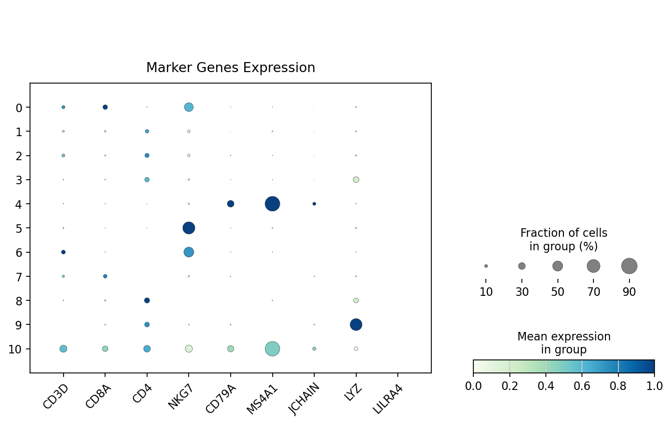

• According to the bubble plot above, cluster 9 may be doublets. This cluster simultaneously expresses markers from different cell types (e.g., T and B cells), showing abnormal co-expression patterns, suggesting cells in this cluster may be doublets of two different types.

Visualization of Cell UMI Count Distribution

Figure Legend: This plot shows the UMI count distribution of all cells, used to identify potential doublets with abnormally high expression.

• X-axis: Order of cells sorted by total UMI count (nCount_RNA) from high to low.
• Y-axis: Log2 transformed total transcript count (nCount_RNA/UMI). Higher values indicate higher detected RNA abundance.
• Middle Scatter Plot: Each dot represents a cell, colors indicate cell groups (Leiden clusters). Cells at the front of the sort order with significantly high UMI counts may represent abnormally high-expressing cells, suggesting potential doublet or multiplet events.
• Top Density Curve: Shows overall nCount_RNA distribution for different cell groups; colors correspond to Leiden clusters, peaks reflect typical RNA abundance levels.
• Right Density Curve: Shows overall distribution of log2(nCount_RNA) by cell group, used to compare RNA abundance differences across cell groups.

warnings.filterwarnings('ignore')
MYCOLOR = None
plot_data = adata_rna.obs[["total_counts", "leiden"]]
plot_data = plot_data.sort_values('total_counts', ascending=False).reset_index(drop=True)
plot_data['order'] = plot_data.index + 1
plot_data['log2_nCount_RNA'] = np.log2(plot_data['total_counts'] + 1)

# Create figure - reduce image size for easier code viewing in Jupyter
fig = plt.figure(figsize=(10, 6), dpi=80) 

# Use GridSpec to place legend on the right to avoid blocking x-axis labels
gs = fig.add_gridspec(2, 3, 
                      width_ratios=[7, 2, 2.5],  # Main plot, right density plot, legend (increase legend area)
                      height_ratios=[2, 6],  # Top density plot, main plot
                      hspace=0.1, wspace=0.1)  # Increase vertical and horizontal spacing to avoid legend crowding the main plot

ax_main = fig.add_subplot(gs[1, 0])
ax_top = fig.add_subplot(gs[0, 0], sharex=ax_main)
ax_right = fig.add_subplot(gs[1, 1], sharey=ax_main)
ax_legend = fig.add_subplot(gs[:, 2])  # Legend placed in the right column

# Hide axis labels
ax_top.tick_params(axis='x', labelbottom=False)
ax_right.tick_params(axis='y', labelleft=False)
ax_top.grid(False)
ax_right.grid(False)

# Get color palette
palette = sns.color_palette('tab20', len(plot_data['leiden'].unique()))
color_map = dict(zip(plot_data['leiden'].unique(), palette))

# 1. Main Scatter Plot
scatter = sns.scatterplot(
    data=plot_data,
    x='order',
    y='log2_nCount_RNA',
    hue='leiden',
    palette=MYCOLOR if MYCOLOR else color_map,
    s=15,
    alpha=0.5,
    edgecolor=None,
    ax=ax_main,
    linewidth=0.5,
    legend=False  # Do not show legend on main plot
)

# Set grid
ax_main.grid(True, linestyle='--', alpha=0.3)
# Set X-axis label
ax_main.set_xlabel('Order(Sorted_by_Total_Counts)', fontsize=12)
ax_main.set_ylabel('log2(Total_Counts)', fontsize=12)

# 2. Top Density Plot (Truncate parts less than 0)
for celltype, color in color_map.items():
    celltype_data = plot_data[plot_data['leiden'] == celltype]
    
    # Calculate density
    if len(celltype_data) > 1:
        from scipy.stats import gaussian_kde
        # Use KDE to calculate density
        kde = gaussian_kde(celltype_data['order'])
        x_density = np.linspace(celltype_data['order'].min(), celltype_data['order'].max(), 200)
        y_density = kde(x_density)
        
        # Normalize density values and truncate negative values
        y_density = np.maximum(y_density, 0)
        
        # Draw fill (starting from 0)
        ax_top.fill_between(x_density, 0, y_density, 
                           color=color, alpha=0.5)
        
        # Draw density line
        ax_top.plot(x_density, y_density, 
                   color=color, alpha=0.7, linewidth=1)

# Set y-axis lower limit of top density plot to 0
ax_top.set_ylim(bottom=0)
ax_top.set_ylabel('Density', fontsize=12)

# 3. Right Density Plot (Truncate parts less than 0)
for celltype, color in color_map.items():
    celltype_data = plot_data[plot_data['leiden'] == celltype]
    
    # Calculate density
    if len(celltype_data) > 1:
        from scipy.stats import gaussian_kde
        # Use KDE to calculate density
        kde = gaussian_kde(celltype_data['log2_nCount_RNA'])
        y_density = np.linspace(celltype_data['log2_nCount_RNA'].min(), 
                               celltype_data['log2_nCount_RNA'].max(), 200)
        x_density = kde(y_density)
        
        # Normalize density values and truncate negative values
        x_density = np.maximum(x_density, 0)
        
        # Draw fill (starting from 0)
        ax_right.fill_betweenx(y_density, 0, x_density, 
                              color=color, alpha=0.5)
        
        # Draw density line
        ax_right.plot(x_density, y_density, 
                     color=color, alpha=0.7, linewidth=1)

# Set x-axis lower limit of right density plot to 0
ax_right.set_xlim(left=0)
ax_right.set_xlabel('Density', fontsize=12)

# 4. Create Legend at Bottom
# Get unique leiden values and corresponding colors
unique_labels = plot_data['leiden'].unique()
leiden_labels = sorted(unique_labels, key=lambda x: int(x))
colors = [color_map[label] for label in leiden_labels]

# Create handles for legend
handles = [plt.Line2D([0], [0], marker='o', color='w', 
                      markerfacecolor=color, markersize=4, 
                      label=label, alpha=0.7) 
           for label, color in zip(leiden_labels, colors)]

# Calculate number of legend columns (auto-adjust based on leiden count)
n_cols = min(8, len(leiden_labels))  # Maximum 8 columns

# Create legend on the right axis
ax_legend.axis('off')  # Turn off axis for the right axis
# Place legend on the right to leave more space
legend = ax_legend.legend(handles=handles, 
                         loc='center left',  # Left centered
                         bbox_to_anchor=(0.1, 0.5),  # Legend position, leave left margin
                         ncol=1,  # Single column display
                         fontsize=12,
                         title='Cluster',
                         title_fontsize=12,
                         frameon=False,
                         fancybox=True,
                         framealpha=0.8,
                         alignment='left')

# Adjust layout - Legend on the right, no extra bottom margin needed
plt.tight_layout(rect=[0, 0.05, 1, 0.95])  # Normal margin
plt.show()
# Limit image display size to avoid filling the entire view
plt.rcParams['figure.max_open_warning'] = 0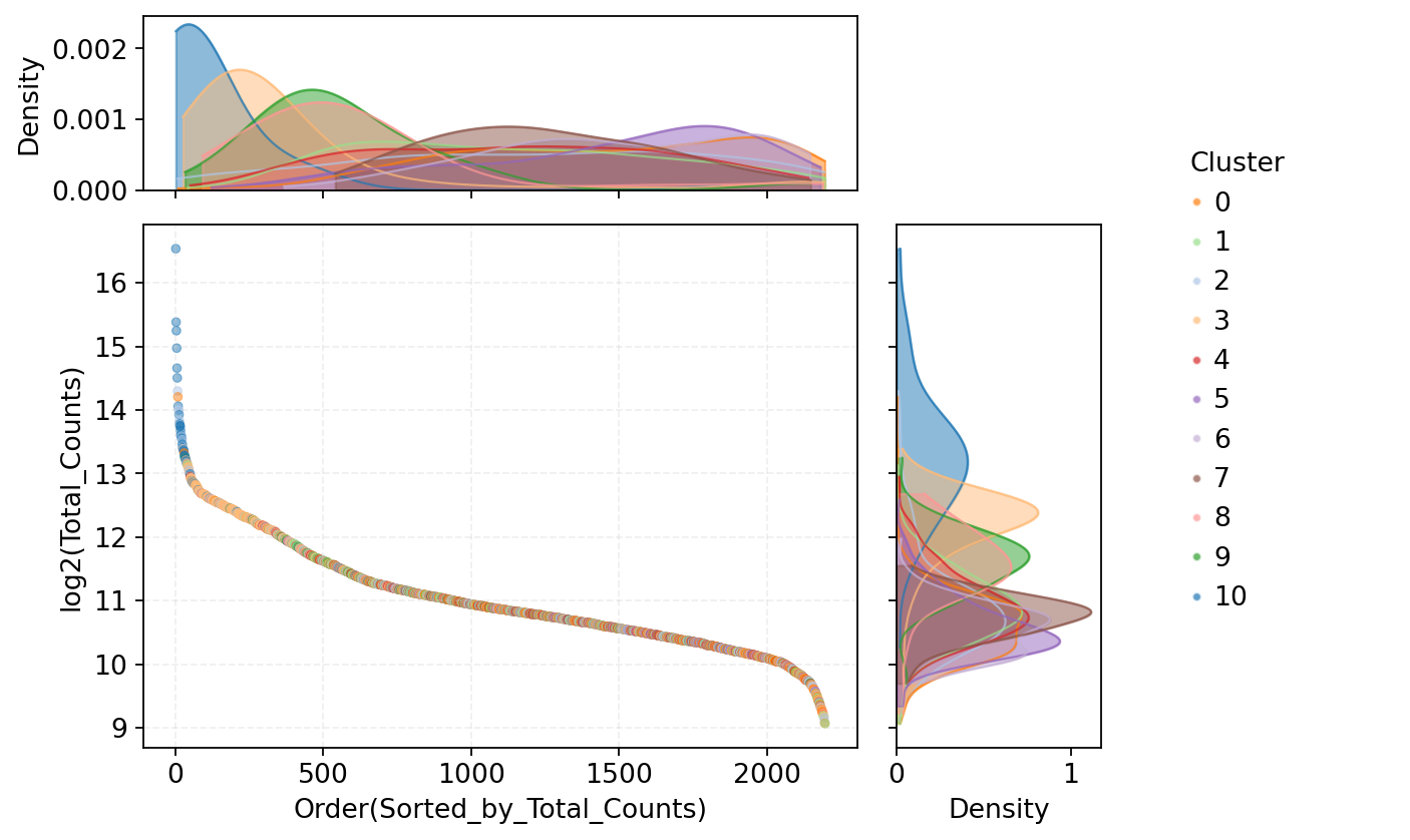

Method 2: Doublet Identification Based on Methylation Reads Count

Principle Explanation:

Since doublets contain DNA from two cells, their methylation sequencing depth (Reads count) is typically significantly higher than single cells. Analyzing Reads count distribution in single-cell methylation data helps identify potential doublets with abnormally high sequencing coverage.

Judgment Logic:

• Doublet Reads counts are usually significantly higher than the average of single cells of the same type, ideally approaching twice the single-cell Reads count.
• In the distribution plot sorted by Reads count, doublets tend to cluster in the high Reads count range.
• By setting a reasonable Reads count threshold, cells with abnormally high coverage can be identified and filtered.

# --- Read methylation Reads count file for each cell ---
# Build path based on new file hierarchy: data/{top_dir}/methylation/{demo_dir}/{sample}/split_bams/filtered_barcode_reads_counts.csv
top_dir = sample_path_config[current_sample]['top_dir']
demo_dir = sample_path_config[current_sample]['demo_dir']
reads_count_path = os.path.join('../../',data_root, top_dir, 'methylation', demo_dir, current_sample, 'split_bams', 'filtered_barcode_reads_counts.csv')
read_count = pd.read_csv(reads_count_path, header=0)
# Extract cell type information from RNA data
rna_meta = pd.DataFrame(adata_rna.obs["leiden"])
rna_meta["gex_cb"] = rna_meta.index

TIP

Please select the corresponding execution flow based on the kit type used:

DD-MET5 Kit:

• Skip the cell below (DD-MET3 specific).
• Directly run the if reagent_type == "DD-MET3"... code in the subsequent cells.

DD-MET3 Kit:

• Must run the cell below first (read Barcode mapping file and merge).
• Then run the subsequent if reagent_type == "DD-MET3"... code.

# --- Read Barcode mapping file for RNA and methylation data ---
# Please download mapping file to local first: https://github.com/seekgene/SeekSoulMethyl/blob/nf_rna_methy/nf/bin/barcodes/DD-M_bUCB3_whitelist.csv
gex_mc_bc_map = pd.read_csv(
    "DD-M_bUCB3_whitelist.csv",
    index_col=None
)
# Unify Barcode column names
gex_mc_bc_map = gex_mc_bc_map.rename(columns={'m_cb': 'barcode'})
# Merge data: Associate Reads counts with Barcode mapping and cell type information
read_count = read_count.merge(gex_mc_bc_map)

if reagent_type == "DD-MET3":
    read_count = read_count.merge(rna_meta)
elif reagent_type == "DD-MET5":
    rna_meta = rna_meta.rename(columns = {'gex_cb': 'barcode'})
    read_count = read_count.merge(rna_meta)

Visualization of Methylation Reads Count Distribution Per Cell

Figure Legend: This plot shows the methylation Reads count distribution of all cells, used to identify potential doublets with abnormally high sequencing coverage.

• X-axis: Order of cells sorted by total Reads count from high to low.
• Y-axis: Log2 transformed total Reads count per cell. Higher values indicate higher methylation sequencing coverage.
• Middle Scatter Plot: Each dot represents a cell, colors indicate cell types. Cells at the front of the sort order with significantly high Reads counts suggest abnormally high coverage, potentially corresponding to doublet or multiplet events.
• Top Density Curve: Shows overall Reads count distribution for different cell types; colors correspond to cell types, peaks reflect typical sequencing coverage levels.
• Right Density Curve: Shows overall distribution of log2(Reads count) by cell type, used to compare sequencing coverage differences across cell types.

warnings.filterwarnings('ignore')
MYCOLOR = None
read_count = read_count.sort_values('reads_counts', ascending=False).reset_index(drop=True)
read_count['order'] = read_count.index + 1
read_count['log2_reads_counts'] = np.log2(read_count['reads_counts'] + 1)

# Create figure - reduce image size for easier code viewing in Jupyter
fig = plt.figure(figsize=(10, 6), dpi=80)  # Reduce image size, not filling the entire view

# Use GridSpec to place legend on the right to avoid blocking x-axis labels
gs = fig.add_gridspec(2, 3, 
                      width_ratios=[7, 2, 2.5],  # Main plot, right density plot, legend (increase legend area)
                      height_ratios=[2, 6],  # Top density plot, main plot
                      hspace=0.1, wspace=0.1)  # Increase vertical and horizontal spacing to avoid legend crowding the main plot

ax_main = fig.add_subplot(gs[1, 0])
ax_top = fig.add_subplot(gs[0, 0], sharex=ax_main)
ax_right = fig.add_subplot(gs[1, 1], sharey=ax_main)
ax_legend = fig.add_subplot(gs[:, 2])  # Legend placed in the right column
ax_top.grid(False)
ax_right.grid(False)

# Hide axis labels
ax_top.tick_params(axis='x', labelbottom=False)
ax_right.tick_params(axis='y', labelleft=False)

# Get color palette
palette = sns.color_palette('tab20', len(read_count['leiden'].unique()))
color_map = dict(zip(read_count['leiden'].unique(), palette))

# 1. Main Scatter Plot
scatter = sns.scatterplot(
    data=read_count,
    x='order',
    y='log2_reads_counts',
    hue='leiden',
    palette=MYCOLOR if MYCOLOR else color_map,
    s=8,
    alpha=0.7,
    ax=ax_main,
    edgecolor=None,
    linewidth=0.5,
    legend=False  # Do not show legend on main plot
)

# Set grid
ax_main.grid(True, linestyle='--', alpha=0.3)
# Set X-axis label
ax_main.set_xlabel('Order(Sorted_by_Reads_Counts)', fontsize=12)
ax_main.set_ylabel('log2(Reads_Counts)', fontsize=12)

# 2. Top Density Plot (Truncate parts less than 0)
for celltype, color in color_map.items():
    celltype_data = read_count[read_count['leiden'] == celltype]
    
    # Calculate density
    if len(celltype_data) > 1:
        from scipy.stats import gaussian_kde
        # Use KDE to calculate density
        kde = gaussian_kde(celltype_data['order'])
        x_density = np.linspace(celltype_data['order'].min(), celltype_data['order'].max(), 200)
        y_density = kde(x_density)
        
        # Normalize density values and truncate negative values
        y_density = np.maximum(y_density, 0)
        
        # Draw fill (starting from 0)
        ax_top.fill_between(x_density, 0, y_density, 
                           color=color, alpha=0.5)
        
        # Draw density line
        ax_top.plot(x_density, y_density, 
                   color=color, alpha=0.7, linewidth=1)

# Set y-axis lower limit of top density plot to 0
ax_top.set_ylim(bottom=0)
ax_top.set_ylabel('Density', fontsize=12)

# 3. Right Density Plot (Truncate parts less than 0)
for celltype, color in color_map.items():
    celltype_data = read_count[read_count['leiden'] == celltype]
    
    # Calculate density
    if len(celltype_data) > 1:
        from scipy.stats import gaussian_kde
        # Use KDE to calculate density
        kde = gaussian_kde(celltype_data['log2_reads_counts'])
        y_density = np.linspace(celltype_data['log2_reads_counts'].min(), 
                               celltype_data['log2_reads_counts'].max(), 200)
        x_density = kde(y_density)
        
        # Normalize density values and truncate negative values
        x_density = np.maximum(x_density, 0)
        
        # Draw fill (starting from 0)
        ax_right.fill_betweenx(y_density, 0, x_density, 
                              color=color, alpha=0.5)
        
        # Draw density line
        ax_right.plot(x_density, y_density, 
                     color=color, alpha=0.7, linewidth=1)

# Set x-axis lower limit of right density plot to 0
ax_right.set_xlim(left=0)
ax_right.set_xlabel('Density', fontsize=12)

# 4. Create Legend at Bottom
# Get unique leiden values and corresponding colors
unique_labels = plot_data['leiden'].unique()
leiden_labels = sorted(unique_labels, key=lambda x: int(x))
colors = [color_map[label] for label in leiden_labels]

# Create handles for legend
handles = [plt.Line2D([0], [0], marker='o', color='w', 
                      markerfacecolor=color, markersize=4, 
                      label=label, alpha=0.7) 
           for label, color in zip(leiden_labels, colors)]

# Calculate number of legend columns (auto-adjust based on leiden count)
n_cols = min(8, len(leiden_labels))  # Maximum 8 columns

# Create legend on the right axis
ax_legend.axis('off')  # Turn off axis for the right axis
# Place legend on the right to leave more space
legend = ax_legend.legend(handles=handles, 
                         loc='center left',  # Left centered
                         bbox_to_anchor=(0.1, 0.5),  # Legend position, leave left margin
                         ncol=1,  # Single column display
                         fontsize=12,
                         title='Clusters',
                         title_fontsize=12,
                         frameon=False,
                         fancybox=True,
                         framealpha=0.8,
                         alignment='left')

# Adjust layout - Legend on the right, no extra bottom margin needed
plt.tight_layout(rect=[0, 0.05, 1, 0.95])  # Normal margin
plt.show()
# Limit image display size to avoid filling the entire view
plt.rcParams['figure.max_open_warning'] = 0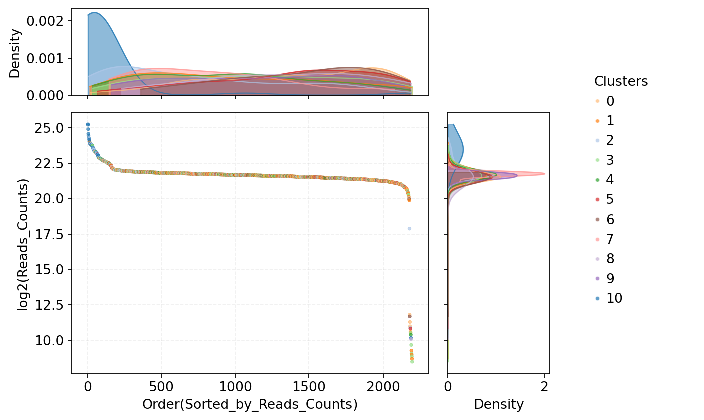

Analysis of Relative Changes in Cell Reads Count

Figure Legend: This plot shows the relative change analysis of cell Reads counts, used to identify inflection points in the Reads count distribution, thereby determining screening thresholds for doublets and low-quality cells.

• X-axis: Order of cells sorted by total Reads count from high to low. Left side are cells with abnormally high Reads, right side are cells with low Reads, middle corresponds to cells with moderate coverage.
• Y-axis: Relative change magnitude in Reads count between adjacent sorted cells, defined as (pre - post) / pre. Values near 0 indicate small changes, larger values indicate significant changes.
• Red Dashed Lines: Selected Reads count threshold range. Left threshold excludes abnormally high Reads cells (potential doublets), right threshold excludes low-quality cells with low Reads. Cells between lines show stable Reads counts suitable for analysis.

# --- Prepare data: Sort by Reads count in descending order ---
p4_data = read_count.copy()

# Sort by reads_counts in descending order
p4_data = p4_data.sort_values('reads_counts', ascending=False).reset_index(drop=True)
p4_data['order'] = p4_data.index + 1

# --- Calculate relative change of adjacent cells: value = (pre - post) / pre ---
plot_df = pd.DataFrame({
    'order': range(1, len(p4_data)),
    'value': (p4_data['reads_counts'].iloc[:-1].values - p4_data['reads_counts'].iloc[1:].values) / 
             p4_data['reads_counts'].iloc[:-1].values
})

# --- Visualize relative change distribution of Reads counts (with LOESS smoothing) ---
plt.figure(figsize=(8, 6), dpi=70) 
# Raw Data Line Plot
plt.plot(plot_df['order'], plot_df['value'], alpha=0.7, linewidth=1, label='Raw data')

# LOESS Smoothing (Simulated using moving average)
span = 0.1
window_size = max(1, int(len(plot_df) * span))
smoothed = plot_df['value'].rolling(window=window_size, center=True, min_periods=1).mean()

# Draw smoothed curve
plt.plot(plot_df['order'], smoothed, color='red', linewidth=1.5, label='LOESS Smoothed')

# Add threshold lines (adjust according to actual situation)
plt.axvline(x=200, linestyle='--', color='red', alpha=0.7, label='High Reads Threshold')
plt.axvline(x=2000, linestyle='--', color='red', alpha=0.7, label='Low Reads Threshold')

plt.xlabel('Order(Sorted_by_Reads_Count)', fontsize=12)
plt.ylabel('Relative_Difference\n(pre-post)/pre', fontsize=12)
plt.title('Reads Distribution with LOESS Smoothing', fontsize=12)
plt.legend(fontsize=12)
plt.grid(True, alpha=0.3)
plt.tight_layout()
plt.show()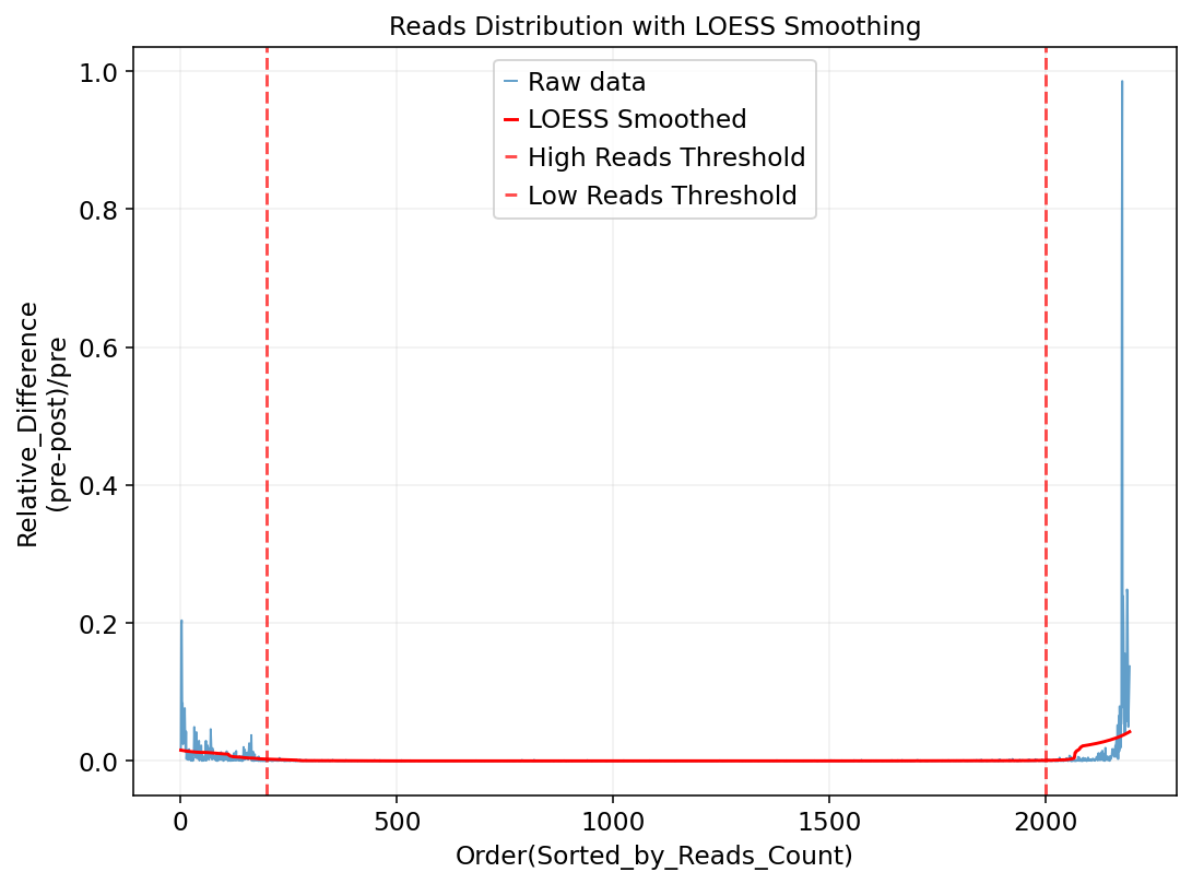

High/Low Reads Cell UMAP Highlighting

Figure Legend: This plot highlights potential doublets and empty cells in UMAP space, used to evaluate the spatial distribution characteristics of these abnormal cells in the cell atlas.

• Left Plot (Potential Multi-Cells): Highlights potential doublets in UMAP space. Red dots indicate top 200 cells with highest Reads counts (candidate doublets), light gray dots indicate other normal cells. Evaluating red dot distribution helps determine if potential doublets cluster in specific regions or are dispersed.
• Right Plot (Potential Empty Cells): Highlights potential empty cells in UMAP space. Red dots indicate the bottom 200 cells with lowest Reads counts (candidate empty cells), light gray dots indicate other normal cells. Used to evaluate spatial distribution patterns of potential empty cells and determine if they correspond to specific low-quality cell populations.

warnings.filterwarnings('ignore')
# --- Identify potential doublets and empty cells based on Reads count threshold ---
# Get 1000 cells with highest Reads counts (potential doublets)
multi_cells = p4_data.head(200)['barcode'].tolist()

# Get 1000 cells with lowest Reads counts (potential empty cells)
empty_cells = p4_data.tail(200)['barcode'].tolist()

# --- Create marker column in AnnData ---
adata_methy.obs['cell_multi_highlight'] = 'other'
adata_methy.obs['cell_empty_highlight'] = 'other'
adata_methy.obs.loc[adata_methy.obs.index.isin(multi_cells), 'cell_multi_highlight'] = 'multi_cells'
adata_methy.obs.loc[adata_methy.obs.index.isin(empty_cells), 'cell_empty_highlight'] = 'empty_cells'

# --- Visualize distribution of potential doublets and empty cells in UMAP space ---
fig, (ax1, ax2) = plt.subplots(1, 2, figsize=(12, 5), dpi=80)

# Subplot 1: Highlight potential doublets (Red)
sc.pl.umap(
    adata_methy, 
    color='cell_multi_highlight', 
    palette={'multi_cells': 'red', 'other': 'lightgrey'},
    ax=ax1,
    s=25,
    show=False,
    title='Potential Multi-Cells (High Read Counts)'
)

# Subplot 2: Highlight potential empty cells (Red)
sc.pl.umap(
    adata_methy, 
    color='cell_empty_highlight', 
    palette={'empty_cells': 'red', 'other': 'lightgrey'},
    ax=ax2, 
    s=25,
    show=False,
    title='Potential Empty Cells (Low Read Counts)'
)

plt.tight_layout()
plt.show()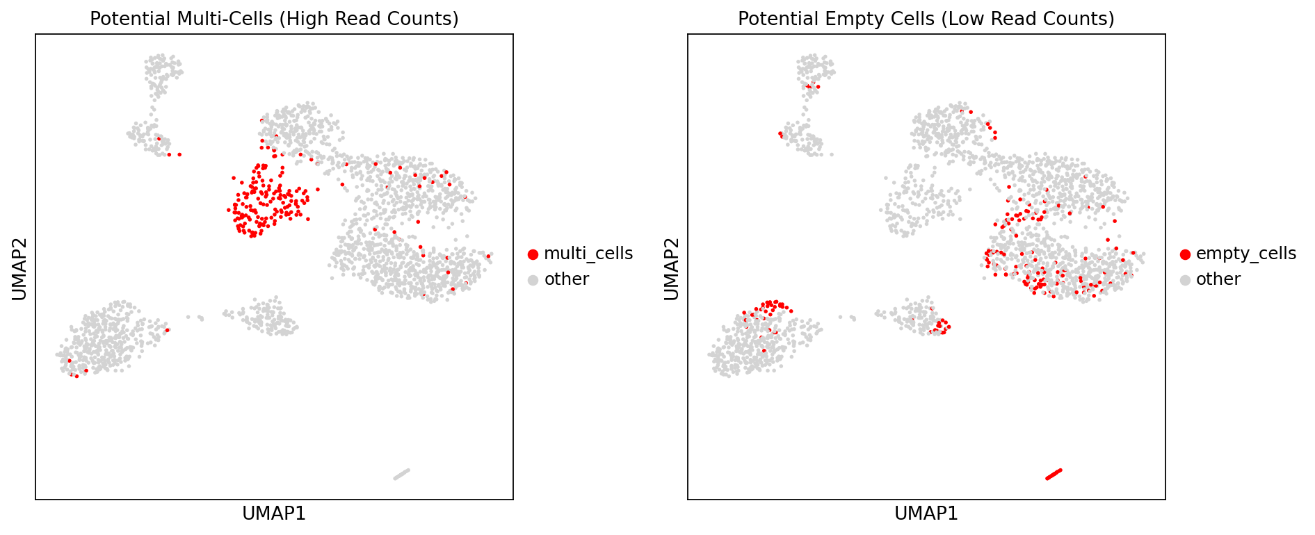

# --- Map RNA annotations to methylation data based on kit type ---
if reagent_type == "DD-MET3":
    # DD-MET3: Map annotations to adata_methyl via map table
    # gex_mc_bc_map contains: g_cb (RNA barcode) and barcode (Methylation barcode, formerly m_cb)
    # Create DataFrame for RNA annotation
    rna_annotation = pd.DataFrame({
        'g_cb': adata_rna.obs.index,
        'rna_leiden': adata_rna.obs['leiden'].values
    })
    
    # Associate RNA annotation to methylation barcode via mapping table
    # gex_mc_bc_map: g_cb -> barcode (Methylation barcode)
    annotation_map = rna_annotation.merge(
        gex_mc_bc_map[['g_cb', 'barcode']],
        on='g_cb',
        how='inner'
    )
    
    # Create Series indexed by methylation barcode
    leiden_series = annotation_map.set_index('barcode')['rna_leiden']
    
    # Add rna_leiden to adata_methy (only add matched cells)
    adata_methy.obs['rna_leiden'] = leiden_series.reindex(adata_methy.obs.index)
    
elif reagent_type == "DD-MET5":
    # DD-MET5: Map directly via barcode equality
    # RNA and methylation barcodes match completely, can map directly via index
    adata_methy.obs['rna_leiden'] = adata_rna.obs.loc[adata_methy.obs.index, 'leiden'].values
else:
    print(f"警告：未知的reagent_type: {reagent_type}")

Comprehensive Doublet Determination

Comprehensive Determination Strategy:

Jointly determine doublets by integrating RNA transcriptome clustering results and methylation Reads count information:

• RNA Transcriptome Determination: Identifies cell populations with abnormal marker gene co-expression characteristics based on RNA data Leiden clustering results. When cells in a cluster (e.g., cluster 9) co-express marker genes from different cell types, that cluster is defined as a potential RNA doublet cluster.

• Methylation Reads Count Determination: Since doublets contain DNA from two cells, their methylation sequencing depth (Reads count) is usually significantly higher than single cells, often concentrating in the high Reads count range in the distribution.

• Comprehensive Determination: Map RNA transcriptome Leiden clustering labels (rna_leiden) to methylation data. For cells with specific rna_leiden values (e.g., 9), combine with their position in the methylation Reads count distribution for joint determination.

  *   Cells are finally identified as doublets when they simultaneously meet the following conditions:
          Potential doublet clusters identified at the RNA level, located in high coverage regions in methylation reads distribution.
  

# --- Mark rna_doublet: When rna_leiden is 9, mark as "doublet" ---
if 'rna_leiden' in adata_methy.obs.columns:
    # Initialize rna_doublet column, default to empty string or 'singlet'
    adata_methy.obs['rna_doublet'] = 'singlet'
    # When rna_leiden is 9 (handling string or numeric types), mark as "rna_doublet"
    adata_methy.obs.loc[adata_methy.obs['rna_leiden'].astype(str) == '9', 'rna_doublet'] = 'doublet'

Method 3: Doublet Identification by Methylation Rate

Use the MethylScrublet algorithm to identify potential doublets. This algorithm simulates artificial doublets and compares them with observed data to calculate a "doublet score" for each cell.

# --- Open MCDS format methylation data (1Mb resolution, for MethylScrublet) ---
# Build path based on new file hierarchy: data/{top_dir}/methylation/{demo_dir}/{sample}/allcools_generate_datasets/{sample}.mcds
top_dir = sample_path_config[current_sample]['top_dir']
demo_dir = sample_path_config[current_sample]['demo_dir']
mcds_path = os.path.join('../../',data_root, top_dir, 'methylation', demo_dir, current_sample, 'allcools_generate_datasets', f'{current_sample}.mcds')
mcds = MCDS.open(
    mcds_path,
    obs_dim="cell",
    var_dim="chrom1M"
)

# --- Extract methylation count (mc) and coverage (cov) matrices ---
mc = mcds[f'chrom1M_da'].sel({'count_type': 'mc'})
cov = mcds[f'chrom1M_da'].sel({'count_type': 'cov'})

# --- If data size is small, load into memory to improve calculation speed ---
load = True
if load and (mcds.get_index('cell').size <= 20000):
    mc.load()
    cov.load()

# --- Initialize MethylScrublet object ---
scrublet = MethylScrublet(
    sim_doublet_ratio=2.0,  # Simulated doublet count = Real cell count * 2.0
    n_neighbors=10,  # KNN Neighbors
    expected_doublet_rate=0.06,  # Expected doublet rate
    stdev_doublet_rate=0.02,  # Standard deviation of doublet rate
    metric='euclidean',  # Distance metric method
    random_state=0,  # Random seed (ensure reproducibility)
    n_jobs=-1  # Use all available CPU cores
)

# --- Run doublet identification algorithm ---
# clusters=None means do not use prior cell type information
score, judge = scrublet.fit(mc, cov, clusters=None)

# --- Save results to AnnData object ---
adata_methy.obs['met_doublet_score'] = score  # Doublet score (0-1, higher means more likely doublet)
adata_methy.obs['met_is_doublet'] = judge  # Doublet determination result (True/False)

# --- Convert identification results to categorical type ---
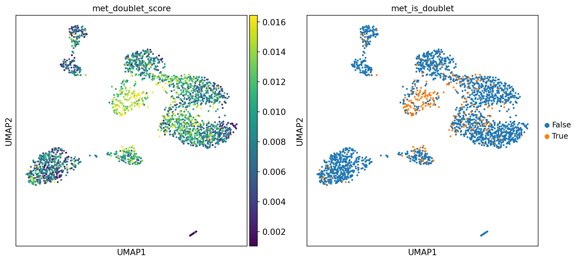
adata_methy.obs['met_is_doublet'] = adata_methy.obs['met_is_doublet'].astype('category')

output

Calculating mC frac of observations...n Simulating doublets...n PCA...n Calculating doublet scores...n Automatically set threshold to 0.01
Detected doublet rate = 12.4%
Estimated detectable doublet fraction = 56.6%
Overall doublet rate:
Expected = 6.0%
Estimated = 21.9%

Figure Legend: This plot displays the doublet identification results of the MethylScrublet algorithm, including doublet score distribution and final determination.

• Left Plot (met_doublet_score): Distribution of doublet scores. Brighter color (yellow) indicates higher similarity to simulated doublet features and higher probability of being a doublet.
• Right Plot (met_is_doublet): Doublet determination results.
  • Orange Points (True): Identified as doublets.
  • Blue Points (False): Identified as normal singlets.

warnings.filterwarnings('ignore')
# --- Set plot parameters ---
sc.set_figure_params(scanpy=True, fontsize=12, facecolor='white', figsize=(6, 6))
# --- Visualize doublet scores and identification results in UMAP space ---
sc.pl.umap(
    adata_methy, 
    color=['met_doublet_score', 'met_is_doublet'], 
    ncols=2,
    s=30
)

adata_methy.obs["m_cb"] = adata_methy.obs.index
# Output doublet identification result file: {sample}_doublet.txt
output_file = f"{current_sample}_doublet.txt"
# Save columns: m_cb, met_is_doublet, cell_multi_highlight, rna_doublet
adata_methy.obs[["m_cb","met_is_doublet","cell_multi_highlight","rna_doublet"]].to_csv(output_file, sep="\t", index=None)