scMethyl + RNA Multi-omics: MethSCAn Differential Methylation Analysis
Module Introduction
This module is based on MethSCAn, used for systematic analysis of single-cell methylation data.
MethSCAn is a command-line toolkit supporting preprocessing, quality control, variation region identification, and downstream analysis of single-cell methylation data. By detecting genome-wide methylation variations, it achieves the following core analysis goals:
- VMR Detection: Automatically identifies Variably Methylated Regions (VMRs) between cells, which are often associated with cell type, developmental stage, or disease state.
- Cell Clustering: Clusters cells based on the methylation feature matrix to effectively distinguish different cell types or states, with a methodological approach similar to single-cell RNA-seq clustering.
- Differential Methylation Analysis (DMR Analysis): Identifies Differentially Methylated Regions (DMRs) between different cell populations to characterize cell heterogeneity at the epigenetic level.
Input File Preparation
This module supports starting analysis from the compact_data directory. The compact_data directory is typically generated by the following data preprocessing workflows:
Data Preprocessing Pipeline
- Methylation-aware Alignment and Extraction: Use allcools analysis pipeline for alignment and methylation site extraction, generating
allcfiles containing methylation and unmethylation site information. - Format Conversion: Use
allc_to_bismarkCov.pyto convertallcfiles to bismark coverage format (.covfiles). - Data Preparation: Use
methscan prepareto convert.covfiles to efficientcompact_dataformat for subsequent analysis.
Note:
- Although MethSCAn supports
allcformat input, its processing efficiency is low. It is generally not recommended for direct use in formal analysis; converting to bismark coverage format first is suggested. - In general, the SeekGene Cloud Platform has completed
allc_to_bismarkCov.pyandmethscan preparesteps by default, and you can directly use the existingcompact_datadirectory for analysis.
File Structure Example
compact_data directory structure is as follows:
compact_data/
├── chr1.npz
├── chr2.npz
├── chr3.npz
├── ...
├── chrX.npz
├── column_header.txt
└── cell_stats.csv
MethSCAn Analysis Pipeline
Script Description: The following code is an initialization example for the MethSCAn analysis workflow, including environment configuration, path settings, and helper function definitions for subsequent steps.
options(warn = -1)
# Load required R packages
suppressPackageStartupMessages({
  library(ggplot2)      # Used for data visualization
  library(dplyr)        # Used for data processing
  library(readr)        # Used for reading CSV files
  library(tidyverse)    # Data Organization and Visualization Toolkit
  library(data.table)   # Efficient data reading and processing
  library(irlba)        # Used for iterative PCA (imputing missing values)
  library(Seurat)       # Single-cell Analysis Tools (Version v5)
  library(Matrix)       # Sparse matrix processing
})

# --- Input parameter configuration ---

## methscan_path: MethSCAn command path
# If methscan is in system PATH, set to NULL
# If methscan is in a different environment, specify full path
methscan_path <- "/jp_envs/envs/methscan/bin/methscan"

## outdir: Result output directory
outdir <- "./DMRs"
# Create output directory (if not exists)
dir.create(outdir, recursive = TRUE, showWarnings = FALSE)

## compact_data_dir: compact_data directory (generated by methscan prepare)
compact_data_dir <- file.path("../../data/AY1768874914782/methylation/demoWTJW969-task-1/WTJW969/methscan/compact_data")

## n_threads: Parallel calculation thread count
# Note: MethSCAn automatically detects the system's maximum thread count; setting n_threads higher than the system maximum will cause an error
# Recommended to set less than or equal to the number of available CPU cores
n_threads <- 8

# Define function: Call MethSCAn command in R
run_methscan <- function(command, args = character(), methscan_path = NULL) {
  # Determine command path: Prioritize parameter, then global variable, finally system PATH
  if (is.null(methscan_path) && exists("methscan_path", envir = .GlobalEnv)) {
    methscan_path <- get("methscan_path", envir = .GlobalEnv)
  }
  cmd <- if (is.null(methscan_path)) "methscan" else methscan_path

  cat("执行:", cmd, command, paste(args, collapse = " "), "\n")

  # Create temporary files to capture stdout and stderr
  stdout_file <- tempfile()
  stderr_file <- tempfile()

  # Execute command, capturing output
  result <- system2(
    cmd,
    args = c(command, args),
    wait = TRUE,
    stdout = stdout_file,
    stderr = stderr_file
  )

  return(invisible(result))
}
Key Parameter Settings
This section summarizes key parameters involved in the MethSCAn analysis workflow. These parameters will be called in subsequent methscan filter, methscan scan, methscan matrix, and methscan diff steps to control key behaviors like cell quality filtering, variable region detection, and differential analysis.
methscan filter Parameters
For specific meanings and recommended values of key parameters for low-quality cell filtering (e.g., min_sites, min_meth, max_meth), please refer to the parameter description table before the filtering execution code in Section 3.2.2.
methscan diff Parameters
Key parameters involved in Differentially Methylated Region (DMR) analysis for comparing differences between clusters are as follows:
| Parameter Name | Chinese Meaning | Default Value | Detailed Description |
|---|---|---|---|
min_cells | Min Cells Requirement | 6 | QC Parameter. Requires region to have coverage in at least this many cells per group for differential analysis. E.g., 6 means only regions covered in >=6 cells per group are tested. Note: Filters low-coverage regions, improving DMR stability. Can lower for small groups but may increase false positives. |
threads Parameter (General Parameter)
Used to control parallel calculation threads for compute-intensive steps (e.g., scan, matrix, diff).
| Parameter Name | Chinese Meaning | Default/Suggested Value | Detailed Description |
|---|---|---|---|
threads | Parallel Calculation Threads | 8 | Performance Optimization Parameter. Accelerates compute-intensive steps (e.g., scan, matrix, diff). Recommended to set based on available CPU cores.Important: MethSCAn automatically detects system max threads. Program errors if threads > system max. Recommended to set <= available CPU cores. |
Best Practice Recommendations
Choice of
methscan filterparameters:**Before parameter setting, it is strongly recommended to run the quality assessment step (see Section 3.2.1)** to identify potential outlier cells by visualizing the distribution of methylation sites and global methylation percentage, and determine the range of `min_sites`, `min_meth`, and `max_meth` accordingly. `min_sites` parameter strategy: When the number of cells retained after filtering is small, this threshold can be appropriately lowered (e.g., to 20000), but may introduce more noise; in cases of high data quality, the threshold can be appropriately raised to enhance result reliability. Global methylation percentage thresholds (`min_meth` and `max_meth`): Global methylation levels usually differ between species, for example: * Mouse: Usually 70-80%. * Human: Usually 60-70%.About Computational Resources:
`methscan scan`, `matrix`, `diff`: Default use of 8c64g resources. **Under common data scales, the entire run usually takes 1-2 hours**. If running in the SeekGene Cloud Platform environment, it is recommended to reserve a longer task time window appropriately.About
min_cellsparameter for DMR analysis:Default value: 6 cells per group Parameter function: Requires a sufficient number of cells in each comparison group to have sequencing coverage in a certain region, thereby improving the statistical stability of differential methylation analysis. Experience reference: In practice, when the number of cells in both comparison clusters is greater than about 200, it is usually easier to obtain DMR results meeting significance thresholds; in cases of fewer cells, it may be difficult to detect significant differences, and one can try appropriately lowering the `min_cells` parameter for exploratory analysis and make a comprehensive judgment based on biological background.
# --- Platform description ---
# In the SeekGene Cloud Platform environment, the methscan prepare step is usually completed in the upstream workflow,
# Therefore, this workflow defaults to directly using the existing compact_data directory.
# The commented code below serves as a reference implementation for local environments or when re-execution of the prepare step is needed;
# If you need to re-run methscan prepare, please uncomment accordingly.


# # Check if input directory exists
# if (!dir.exists(input_cov_dir)) {
#   stop("Input directory does not exist: ", input_cov_dir,
#        "\nPlease run allc_to_bismarkCov.py to convert data first")
# }
#
# # Get all coverage files
# cov_files <- list.files(input_cov_dir, full.names = TRUE, pattern = "\\.cov$")
# if (length(cov_files) == 0) {
#   stop("No .cov files found in ", input_cov_dir)
# }
#
# cat("Found ", length(cov_files), " coverage files\n")
#
# # Prepare output directory
# compact_data_dir <- file.path(outdir, "compact_data")
# if (!dir.exists(compact_data_dir)) {
#   dir.create(compact_data_dir, recursive = TRUE)
# }
#
# # Execute methscan prepare
# run_methscan(
#   command = "prepare",
#   args = c(cov_files, compact_data_dir)
# )

# Directly use existing compact_data directory
if (!dir.exists(compact_data_dir)) {
  stop("compact_data 目录不存在:", compact_data_dir,
       "\n请确保已在云平台完成 methscan prepare 步骤")
}
cat("✓ 使用已有的 compact_data 目录:", compact_data_dir, "\n")Quality Assessment and Low-quality Cell Filtering
Before performing cell filtering, it is recommended to systematically assess cell quality and determine appropriate filtering parameters combined with visualization results.
Cell Statistics Reading and Quality Metric Visualization
# Read cell_stats.csv file
cell_stats_path <- file.path(compact_data_dir, "cell_stats.csv")
cell_stats <- read_csv(cell_stats_path)
#if (file.exists(cell_stats_path)) {
# cell_stats <- read_csv(cell_stats_path)
# cat("Successfully read cell statistics, total", nrow(cell_stats), "cells\n")
# head(cell_stats)
#} else {
# stop("cell_stats.csv file not found, please check if the path is correct")
#}
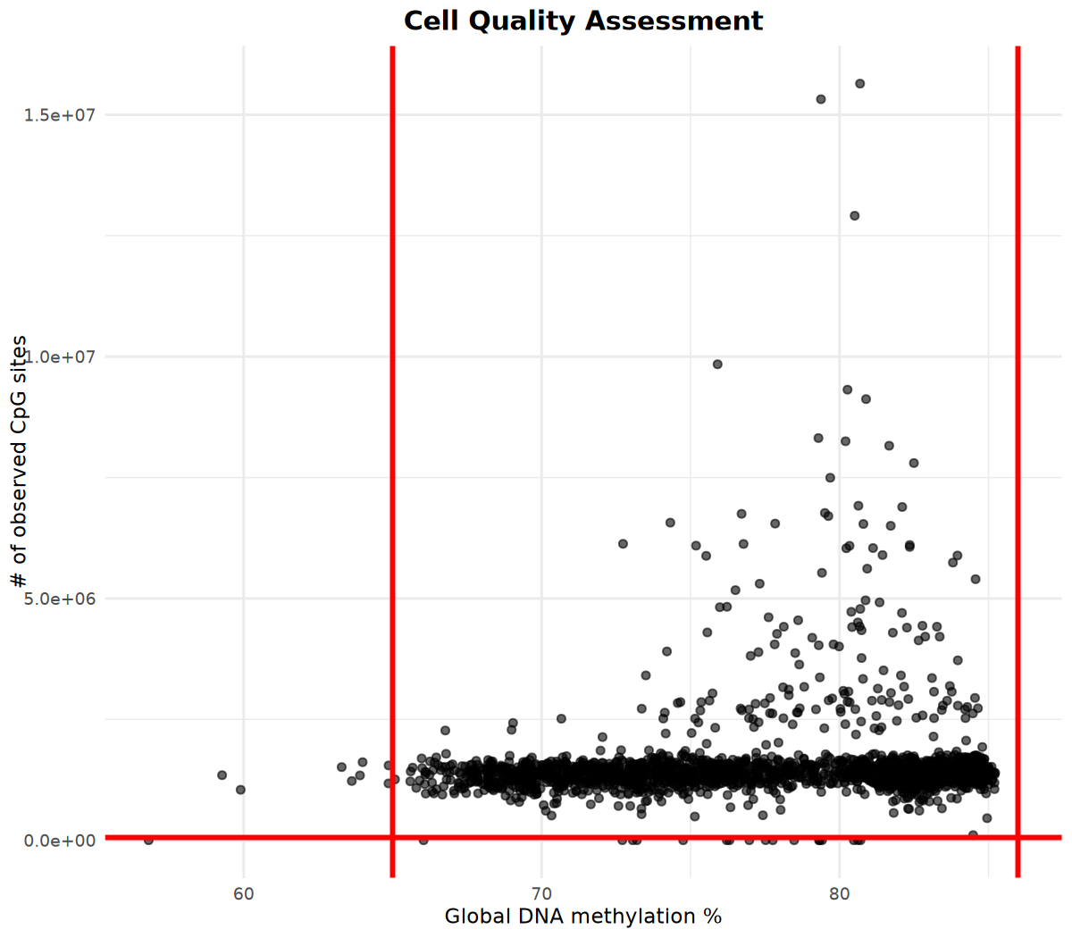
# Visualize number of methylation sites and global methylation percentage
# Determine filtering parameters based on visualization results
options(repr.plot.width = 8, repr.plot.height = 7, repr.plot.res = 150)
p <- cell_stats %>%
ggplot(aes(x = global_meth_frac * 100, y = n_obs)) +
geom_point(alpha = 0.6) +
# Add red vertical lines at x-coordinates 65 and 86 (example thresholds)
geom_vline(xintercept = c(65, 86), color = "red", linetype = "solid", linewidth = 1) +
# Add red horizontal line at y-coordinate 60000 (example threshold)
geom_hline(yintercept = 60000, color = "red", linetype = "solid", linewidth = 1) +
labs(
x = "Global DNA methylation %",
y = "# of observed CpG sites",
title = "Cell Quality Assessment"
) +
theme_minimal() +
theme(
plot.title = element_text(hjust = 0.5, size = 14, face = "bold")
)
print(p)── Column specification ────────────────────────────────────────────────────────
Delimiter: ","
chr (1): cell_name
dbl (3): n_obs, n_meth, global_meth_frac
ℹ Use \`spec()\` to retrieve the full column specification for this data.
ℹ Specify the column types or set \`show_col_types = FALSE\` to quiet this message.
Perform Filtering Based on Visualization Results
Based on the above visualization results, determine filtering parameters and execute cell filtering:
methscan filter Key Parameters:
| Parameter Name | Chinese Meaning | Default/Suggested Value | Detailed Description |
|---|---|---|---|
min_sites | Min Observed Methylation Sites | 25000-60000 | QC Parameter. Requires cell to have > this number of observed methylation sites. Removes low-quality cells with insufficient depth for accurate methylation status inference. Note: Threshold depends on sequencing depth; higher depth allows higher threshold. |
min_meth | Min Global Methylation % | 60-70 | QC Parameter. Requires cell global methylation % > this value. Removes abnormal cells due to incomplete bisulfite conversion or technical issues. Note: Normal levels vary (e.g., Mouse ~70-80%, Human ~60-70%). |
max_meth | Max Global Methylation % | 70-85 | QC Parameter. Requires cell global methylation % < this value. Removes abnormally hypermethylated cells due to technical issues. Note: Normal levels vary by species/cell type; set reasonable thresholds based on data. |
threads | Parallel Calculation Threads | 8 | Accelerates compute-intensive steps (e.g., scan, matrix). Recommended to set based on system resources, usually available CPU cores. |
# Filtering parameters (please adjust based on QC results)
min_sites <- 60000    # Minimum observed methylation sites
min_meth <- 65       # Minimum global methylation percentage
max_meth <- 86        # Maximum global methylation percentage

# Prepare output directory
filtered_data_dir <- file.path(outdir, "filtered_data")
if (!dir.exists(filtered_data_dir)) {
  dir.create(filtered_data_dir, recursive = TRUE)
}

# Execute methscan filter
run_methscan(
  command = "filter",
  args = c(
    "--min-sites", min_sites,
    "--min-meth", min_meth,
    "--max-meth", max_meth,
    compact_data_dir,
    filtered_data_dir
  )
)Data Smoothing: methscan smooth
Before VMR/DMR detection, methylation data smoothing is required. methscan smooth treats all single cells as pseudo-bulk samples to calculate genome-wide smoothed average methylation levels. This result is a necessary input for subsequent VMR detection and methylation matrix construction.
Output Results: Smoothed result files are output to the ${outdir}/filtered_data/smoothed directory.
# Execute methscan smooth
run_methscan(
  command = "smooth",
  args = filtered_data_dir
)VMR Detection: methscan scan
This step detects Variable Methylation Regions (VMR). methscan scan automatically identifies regions with significant intercellular methylation variation genome-wide.
Output Results: Generates result file in BED format, containing genomic coordinates and methylation variance of VMRs.
Alternative: If the analysis target is limited to specific genomic regions (such as promoters or gene body regions), you can directly provide the corresponding BED file, skip the scan step, and directly use methscan matrix to analyze these regions.
# VMR Output File
vmr_bed_file <- file.path(outdir, "VMRs.bed")

# Execute methscan scan
result <- run_methscan(
  command = "scan",
  args = c(
    "--threads", n_threads,
    filtered_data_dir,
    vmr_bed_file
  )
)VMR Matrix Generation: methscan matrix
This step constructs a methylation matrix based on identified VMR regions for subsequent cell clustering and related downstream analysis.
Output File Description:
The output directory VMR_matrix contains the following files:
| Filename | Description |
|---|---|
mean_shrunken_residuals.csv.gz | Shrunken Residuals Matrix (Recommended for downstream). Less affected by random coverage changes, better for reduction/clustering. |
methylation_fractions.csv.gz | Methylation Fraction Matrix. Methylation fraction (0-1) for each region, representing average methylation level. |
methylated_sites.csv.gz | Methylated Sites Matrix (Numerator). Number of methylated CpG sites in each region. |
total_sites.csv.gz | Total Sites Matrix (Denominator). Total number of CpG sites with sequencing coverage in each region. |
Matrix Features:
- Many missing values: Due to low coverage in single-cell sequencing, some genomic regions may lack valid sequencing reads in some cells, resulting in many missing values.
- Methylation values are in small-denominator fraction form: Methylation levels are usually represented as small-denominator fractions (e.g., 1/1, 2/2, 1/3), a typical feature of single-cell methylation data.
- Additional site statistics: The output directory also contains the number of methylated CpG sites and CpG sites with sequencing coverage for each region, corresponding to the numerator and denominator in methylation ratio calculation respectively.
# VMR Matrix Output Directory
vmr_matrix_dir <- file.path(outdir, "VMR_matrix")

# Execute methscan matrix
result <- run_methscan(
  command = "matrix",
  args = c(
    "--threads", n_threads,
    vmr_bed_file,
    filtered_data_dir,
    vmr_matrix_dir
  )
)

# Check if output files are generated
if (result == 0 && dir.exists(vmr_matrix_dir)) {
  expected_files <- c(
    "mean_shrunken_residuals.csv.gz",
    "methylation_fractions.csv.gz",
    "methylated_sites.csv.gz",
    "total_sites.csv.gz"
  )
  existing_files <- list.files(vmr_matrix_dir)
  found_files <- expected_files[expected_files %in% existing_files]

  if (length(found_files) > 0) {
    cat("✓ VMR 矩阵文件已生成:\n")
    for (f in found_files) {
      file_path <- file.path(vmr_matrix_dir, f)
      file_size <- file.info(file_path)$size / 1024 / 1024  # MB
      cat("  -", f, sprintf("(%.2f MB)\n", file_size))
    }
  } else {
    warning("警告:未找到预期的输出文件,请检查输出目录:", vmr_matrix_dir)
  }
} else if (result != 0) {
  stop("methscan matrix 执行失败,请检查上面的错误信息")
}✓ VMR 矩阵文件已生成:
- mean_shrunken_residuals.csv.gz (291.34 MB)
- methylation_fractions.csv.gz (60.59 MB)
- methylated_sites.csv.gz (43.48 MB)
- total_sites.csv.gz (56.35 MB)
VMR-based Clustering Analysis
This section uses Seurat for dimensionality reduction and clustering analysis based on the VMR methylation matrix to identify cell populations with similar methylation characteristics.
Read VMR Matrix
# Use fread to read compressed files
# Use configured outdir variable
vmr_matrix_path <- file.path(outdir, "VMR_matrix", "mean_shrunken_residuals.csv.gz")

if (file.exists(vmr_matrix_path)) {
  cat("正在读取 VMR 矩阵...\n")
  meth_mtx <- fread(vmr_matrix_path)
  cat("矩阵维度:", nrow(meth_mtx), "行(细胞)x", ncol(meth_mtx) - 1, "列(VMR 区域)\n")

  # Set first column as row names and convert to matrix
  row_names <- meth_mtx[[1]]
  meth_mtx <- as.matrix(meth_mtx[, -1])
  rownames(meth_mtx) <- row_names

  cat("矩阵转换完成!\n")
  cat("缺失值比例:", round(mean(is.na(meth_mtx)) * 100, 2), "%\n")
} else {
  stop("找不到 VMR 矩阵文件,请检查路径是否正确")
}矩阵转换完成!
缺失值比例: 75.31 %
Iterative PCA Imputation
The VMR methylation matrix is structurally similar to the single-cell RNA-seq count matrix, but its distinguishing feature is containing a large number of missing values. This is mainly due to low coverage in single-cell methylation sequencing, resulting in many genomic regions lacking effective sequencing reads in some cells.
To address the missing value issue, this analysis uses an iterative PCA method for imputation. Specifically: missing values are first initialized with 0; then PCA is performed on the filled matrix, and predicted values reconstructed from PCA replace the original 0s; this process repeats iteratively until imputed values stabilize between adjacent iterations.
This method provides more reasonable estimates for missing methylation values by iteratively optimizing low-dimensional structure, providing a more complete and stable data foundation for subsequent dimensionality reduction and clustering analysis.
# Define function for iterative PCA imputation of missing values
prcomp_iterative <- function(x, n = 15, n_iter = 50, min_gain = 0.001, ...) {
  mse <- rep(NA, n_iter)
  na_loc <- is.na(x)
  x[na_loc] <- 0  # zero is our first guess

  for (i in 1:n_iter) {
    prev_imp <- x[na_loc]  # what we imputed in the previous round
    # PCA on the imputed matrix
    pr <- prcomp_irlba(x, center = F, scale. = F, n = n, ...)
    # impute missing values with PCA
    new_imp <- (pr$x %*% t(pr$rotation))[na_loc]
    x[na_loc] <- new_imp
    # compare our new imputed values to the ones from the previous round
    mse[i] <- mean((prev_imp - new_imp) ^ 2)
    # if the values didn't change a lot, terminate the iteration
    gain <- mse[i] / max(mse, na.rm = T)
    if (gain < min_gain) {
      message(paste(c("\n\nTerminated after ", i, " iterations.")))
      break
    }
  }
  message(paste(c("\n\nTerminated after ", i, " iterations. Gain: ", round(gain, 6))))
  pr$mse_iter <- mse[1:i]
  list(pr = pr, imputed_matrix = x)
}

cat("开始执行迭代 PCA 填补缺失值...\n")
result_residual <- meth_mtx %>%
  scale(center = T, scale = F) %>%
  prcomp_iterative(n = 15)

# Extract imputed residual matrix
residual_mtx_imputed <- result_residual$imputed_matrix
cat("缺失值填补完成!\n")Terminated after 32 iterations.
Terminated after 32 iterations. Gain: 0.000974
缺失值填补完成!
Create Seurat Object
Use the imputed residual matrix (residual_mtx_imputed) as input for the Seurat object. When constructing the Seurat object, counts, data, and scale.data matrices all use the same imputed residual matrix.
Explanation: Subsequent PCA, dimensionality reduction, and clustering analysis are actually based on the scale.data matrix.
# Create Seurat object using imputed residual matrix
# counts, data, and scale.data matrices use the same imputed residual matrix
seurat_obj <- CreateSeuratObject(
    counts = as(t(residual_mtx_imputed), "sparseMatrix"),
    project = "MethSCAn",
    assay = "VMR"
)
# Set data and scale.data to the same matrix as counts
# Note: Subsequent PCA, dimensionality reduction, and clustering analysis actually use the scale.data matrix
seurat_obj@assays$VMR@data <- seurat_obj@assays$VMR@counts
seurat_obj@assays$VMR@scale.data <- as.matrix(seurat_obj@assays$VMR@counts)
PCA, UMAP Dimensionality Reduction and Clustering
# 1. PCA Dimensionality Reduction
# Use Seurat's RunPCA function
# This automatically reads data from scale.data layer and calculates PCA
n_pcs = 30
seurat_obj <- RunPCA(
seurat_obj,
features = rownames(seurat_obj), # Use all VMRs
npcs = n_pcs, # Calculate top 30 principal components
assay = "VMR",
verbose = FALSE
)
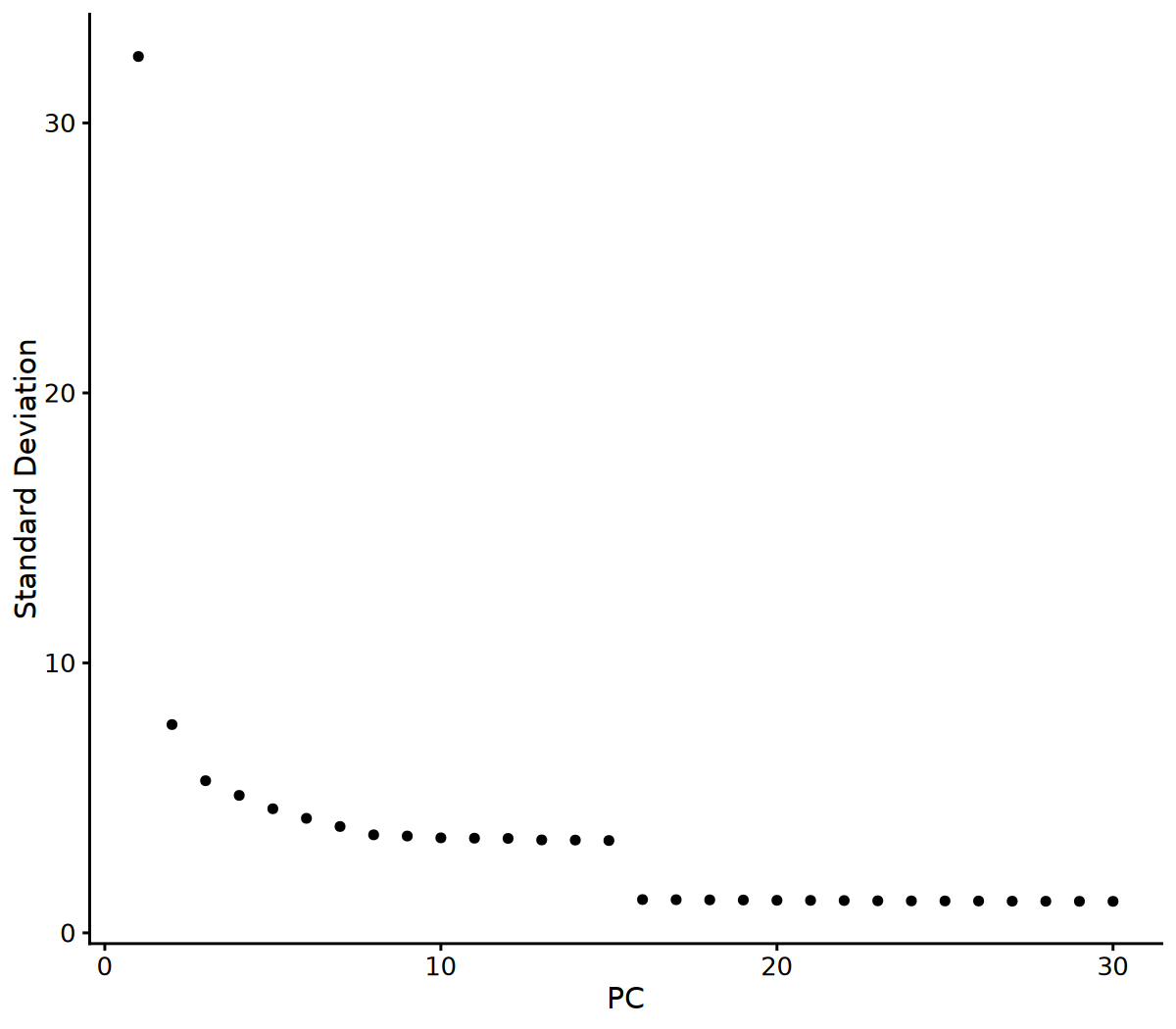
options(repr.plot.width = 8, repr.plot.height = 7, repr.plot.res = 150)
# Visualize Elbow Plot to determine number of PCs
ElbowPlot(seurat_obj, ndims = 30)
# 2. Determine number of PCs based on Elbow Plot
# You can adjust this parameter based on the Elbow Plot results
n_pcs_use <- 10
# 3. UMAP Dimensionality Reduction
seurat_obj <- RunUMAP(seurat_obj, dims = 1:n_pcs_use, reduction = "pca", verbose = FALSE)
cat("UMAP 降维完成!\n")
# 4. Build KNN Graph
seurat_obj <- FindNeighbors(seurat_obj, dims = 1:n_pcs_use, reduction = "pca", verbose = FALSE)
cat("KNN 图构建完成!\n")
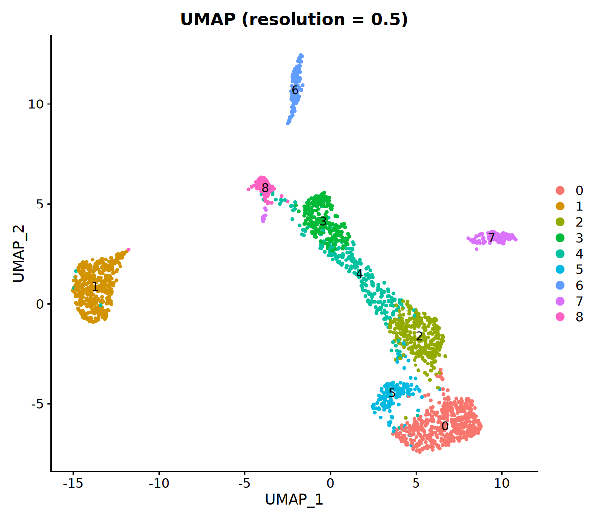
# 5. Clustering (resolution parameter can be adjusted; larger value means more clusters)
seurat_obj <- FindClusters(seurat_obj, resolution = 0.5, verbose = FALSE)
cat("聚类完成!\n")
# 6. Visualize Clustering Results
DimPlot(seurat_obj, group.by = 'VMR_snn_res.0.5', label = TRUE) +
ggtitle("UMAP (resolution = 0.5)")KNN 图构建完成!
聚类完成!
Save Results
# Save Seurat object
output_file <- "MethSCAn.rds"
saveRDS(seurat_obj, file = output_file)clust_tbl <- seurat_obj@meta.data
clust_tbl$cell <- row.names(clust_tbl)
clust_tbl %>%
mutate(cell_group = case_when(
seurat_clusters == "0" ~ "-",
seurat_clusters == "1" ~ "1",
seurat_clusters == "2" ~ "2",
seurat_clusters == "3" ~ "-",
seurat_clusters == "4" ~ "-",
seurat_clusters == "5" ~ "-",
seurat_clusters == "6" ~ "-",
seurat_clusters == "7" ~ "-",
seurat_clusters == "8" ~ "-"
)) %>%
dplyr::select(cell, cell_group) %>%
write_csv("cell_groups.csv", col_names=F)Differential Methylated Region Analysis: methscan diff
Differentially Methylated Region (DMR) analysis compares methylation differences between cells under different conditions, such as different clusters, cell types, or custom groups. It is generally recommended to perform DMR analysis based on clustering results or predefined groups after completing clustering analysis.
Input File Preparation
Input Requirements:
- Data Directory:
filtered_datadirectory (must have completedmethscan smoothstep). - Cell Group File (cell_groups_file): CSV format file, where the first column is cell name (cell barcode) and the second is group label. Label rules:
group_Aandgroup_Brepresent the two cell groups involved in comparison;-represents other cells not participating in this comparison.
File Format Example:
cell_01,-
cell_02,-
cell_03,-
cell_04,group_A
cell_05,group_A
cell_06,group_A
cell_07,group_B
cell_08,group_B
cell_09,group_B# Cell grouping file (for DMR analysis)
cell_groups_file <- "cell_groups.csv" # Please modify according to actual situation
# DMR Output File
dmr_bed_file <- file.path(outdir, "DMRs.bed")
# Check if cell grouping file exists
if (file.exists(cell_groups_file)) {
# Execute methscan diff
run_methscan(
command = "diff",
args = c(
"--threads", n_threads,
filtered_data_dir,
cell_groups_file,
dmr_bed_file
)
)
} else {
warning("细胞分组文件不存在:", cell_groups_file,
"\n跳过 DMR 分析。如需进行 DMR 分析,请先准备细胞分组文件。")
}Output File Format Description
Output File: DMRs.bed
Results are output in BED format, containing the following fields:
| Column No. | Column Name | Description | Example Value |
|---|---|---|---|
| 1 | chromosome | Chromosome name | 17 |
| 2 | DMR_start | DMR start position (genomic coordinate) | 58270529 |
| 3 | DMR_end | DMR end position (genomic coordinate) | 58285529 |
| 4 | t_statistic | Welch's t-test statistic | -12.85232790631932 |
| 5 | n_sites | Total number of methylation sites in this region (CpG count) | 561 |
| 6 | n_cells_group1 | Number of cells with coverage in Group 1 | 150 |
| 7 | n_cells_group2 | Number of cells with coverage in Group 2 | 66 |
| 8 | meth_frac_group1 | Average methylation level of Group 1 (0–1) | 0.3396857458943857 |
| 9 | meth_frac_group2 | Average methylation level of Group 2 (0–1) | 0.8429240842342447 |
| 10 | low_group_label | Label of the group with lower methylation level | group_1 |
| 11 | p | Raw p-value (unadjusted) | 0.0 |
| 12 | adjusted_p | Adjusted p-value (FDR, Benjamini-Hochberg method) | 0.0 |
Result Interpretation: The low_group_label column indicates the group label with lower methylation levels; the adjusted_p column is the significance level after multiple testing correction, usually recommended to use adjusted_p < 0.05 as the screening threshold; the sign of t_statistic indicates the direction of difference (negative value indicates lower methylation in group_1, positive value indicates higher methylation in group_1).
Generate Significant Differential Methylated Region File
Based on the DMRs.bed file, screen for significantly differentially methylated regions (adjusted_p < 0.05), and group results based on low_group_label to generate two BED files.
Input: DMRs.bed: DMR detection result file
Output: Generate the following two significant DMR BED files based on the value of low_group_label:
DMRs_significant_group_A.bed: DMR regions with significantly lower methylation levels in group_A.DMRs_significant_group_B.bed: DMR regions with significantly lower methylation levels in group_B.
The above output files are all in BED format, containing three columns: chromosome, start, end. If chromosome names are numbers or sex chromosomes (X/Y), "chr" prefix is automatically added; if "chr" prefix already exists, it is kept unchanged.
Explanation: Only keep significant DMRs with adjusted_p < 0.05, automatically add "chr" prefix to numeric and sex chromosomes (keep unchanged if already present), and skip rows where low_group_label is empty or "-".
# Generate significant DMR files (grouped by low_group_label, adjusted_p < 0.05)
# Add "chr" prefix to autosomes (numbers) and sex chromosomes (XY)
# Check if DMRs.bed file exists
if (file.exists(dmr_bed_file)) {
  cat("开始生成显著的 DMR 文件...\n")

  # Build awk command
  awk_script <- sprintf('
BEGIN {
    outdir = "%s"
}
# Skip header or empty lines
NR == 1 && $1 ~ /^chromosome|^#/ { next }
NF < 12 { next }
# Filter rows with adjusted_p < 0.05
$12 < 0.05 {
    # Get low_group_label (10th column) as filename
    group_label = $10
    if (group_label == "" || group_label == "-") next

    # Process chromosome names: If numeric or X/Y, add "chr" prefix
    chrom = $1
    if (chrom ~ /^[0-9]+$/ || chrom ~ /^[XY]$/) {
        chrom = "chr" chrom
    }

    # Build output filename
    output_file = outdir "/DMRs_significant_" group_label ".bed"

    # Output first 3 columns (chromosome, start, end) to corresponding file
    print chrom "\\t" $2 "\\t" $3 > output_file
}
END {
    print "处理完成!已生成显著的 DMR 文件。"
}
', outdir)

  # Execute awk command in R
  awk_cmd <- paste("awk -F'\\t'", shQuote(awk_script), shQuote(dmr_bed_file))
  result <- system(awk_cmd, intern = TRUE)

  # Display output
  cat(paste(result, collapse = "\n"), "\n")

  # Check generated files
  significant_files <- list.files(
    path = outdir,
    pattern = "^DMRs_significant_.*\\.bed$",
    full.names = TRUE
  )

  if (length(significant_files) > 0) {
    cat("\n生成的显著 DMR 文件:\n")
    for (f in significant_files) {
      n_lines <- length(readLines(f, warn = FALSE))
      cat("  -", basename(f), "(", n_lines, " 个区域)\n", sep = "")
    }
  } else {
    warning("未找到生成的显著 DMR 文件")
  }
} else {
  warning("DMRs.bed 文件不存在:", dmr_bed_file,
          "\n请先执行 methscan diff 命令")
}生成的显著 DMR 文件:
-DMRs_significant_1.bed(23951 个区域)
-DMRs_significant_2.bed(30189 个区域)