Single-cell Methylation + RNA Dual-omics Multi-sample Integration Analysis Pipeline (ALLCools)

Author: SeekGene

Time: 23 min

Words: 4.5k words

Updated: 2026-03-02

Reads: 0 times

scMethyl + RNA-seq Notebooks

Load Python Analysis Packages

python

import os
import re
import glob
from ALLCools.mcds import MCDS
from ALLCools.clustering import tsne, significant_pc_test, log_scale, lsi, binarize_matrix, filter_regions, cluster_enriched_features, ConsensusClustering, Dendrogram, get_pc_centers
from ALLCools.clustering.doublets import MethylScrublet
from ALLCools.plot import *
import scanpy as sc
import scanpy.external as sce
from harmonypy import run_harmony
import numpy as np
import pandas as pd
import matplotlib.pyplot as plt
import matplotlib.colors as mcolors
from matplotlib.lines import Line2D
import warnings
import xarray as xr
from ALLCools.clustering import one_vs_rest_dmg
import pybedtools
from scipy import sparse

python

samples = ["HC10_12","HC14_21"]
var_dim = 'chrom20k'
obs_dim = 'cell'
mc_type = 'CGN'
quant_type = 'hypo-score'

Input Folder Structure

text

HC10_12
├── HC10_12_exp
│   └── HC10_12
│       └── Analysis
│            └── step3
│                ├── filtered_feature_bc_matrix
│                └── raw_feature_bc_matrix
└── HC10_12_methy
    └── step3
        ├── allcools_generate_datasets
        └── split_BAMs
            ├── filtered_barcode_reads_counts.csv
            └── HC10_12_cells.csv

⚠️ Important Note
This tutorial applies to the above directory structure. If your file organization is different, please adjust folder paths or modify file addresses in the code accordingly.

⚠️ Important Note
If the reagent type is DD-MET3, you need to read the correspondence.

python

gex_mc_bc_map = pd.read_csv("/PROJ2/FLOAT/weiqiuxia/project/20241227_methy/script/SeekSoulMethyl/nf/bin/barcodes/DD-M_bUCB3_whitelist.csv",index_col=None)

Single-cell RNA Sequencing Data Multi-sample Integration Analysis Pipeline

Data Preprocessing Pipeline

Normalization and Transformation

Count Normalization
Uses total count normalization to eliminate sequencing depth differences between cells, ensuring fair comparison.
Variance Stabilizing Transformation
Applies logarithmic transformation (log1p) so that highly expressed genes do not overly dominate analysis results.

Feature Gene Selection

Identifies 2000 highly variable genes via statistical methods; these genes show significant expression differences between cells and are most likely to reflect important biological signals.

Batch Effect Correction

Application of Harmony Algorithm

Uses the advanced Harmony ensemble learning method to elegantly resolve technical variations between multiple samples:

Cell Atlas Construction

Neighborhood Relationship Calculation

Based on the corrected feature space, constructs a k-nearest neighbor graph (k=30) of cells to quantify similarity relationships.

Clustering Analysis

Uses the Leiden algorithm for cell population identification; this algorithm discovers high-quality community structures. Resolution parameter is set to 0.5 for moderate clustering granularity.

Visualization

UMAP Dimensionality Reduction
Preserves data topology, providing an intuitive view of cell distribution.

python


# Read Expression data and add meta data to RNA and MET data
obj_rna_list = {}
    
for i in samples:
    s_rna_path = os.path.join(f'{i}', f'{i}_exp',f'{i}', 'Analysis', 'step3', 'filtered_feature_bc_matrix')      
    obj_rna_list[i] = sc.read_10x_mtx(s_rna_path)
    #obj_rna_list[i].obs['batch']=f'{i}'

adata_rna=obj_rna_list[samples[0]].concatenate([obj_rna_list[i] for i in samples[1:] ])
adata_rna.obs['Sample'] = adata_rna.obs['batch'].map(
    {f'{index}': value for index, value in enumerate(samples)}
)
sc.pp.normalize_total(adata_rna, inplace=True)
sc.pp.log1p(adata_rna)
sc.pp.highly_variable_genes(adata_rna, n_bins=100, n_top_genes=2000)
adata_rna.raw = adata_rna
adata_rna = adata_rna[:, adata_rna.var.highly_variable]
sc.pp.scale(adata_rna, max_value=10)
sc.tl.pca(adata_rna)
ho = run_harmony(adata_rna.obsm['X_pca'],
                 meta_data=adata_rna.obs,
                 vars_use='Sample',
                 random_state=0,
                 max_iter_harmony=20)
adata_rna.obsm['X_pca_harmony'] = ho.Z_corr.T
reduc_use = 'X_pca_harmony'
sc.pp.neighbors(adata_rna,n_neighbors=30,use_rep = reduc_use)
sc.tl.umap(adata_rna)
sc.tl.tsne(adata_rna,use_rep=reduc_use)
sc.tl.leiden(adata_rna, resolution=0.5)

output

RNA Single-modality Cell Annotation

python

marker_names = ["CD3D","NKG7","CD8A","CD4","CD79A","MS4A1","JCHAIN","LYZ","LILRA4"]
sc.pl.umap(adata_rna,color = marker_names)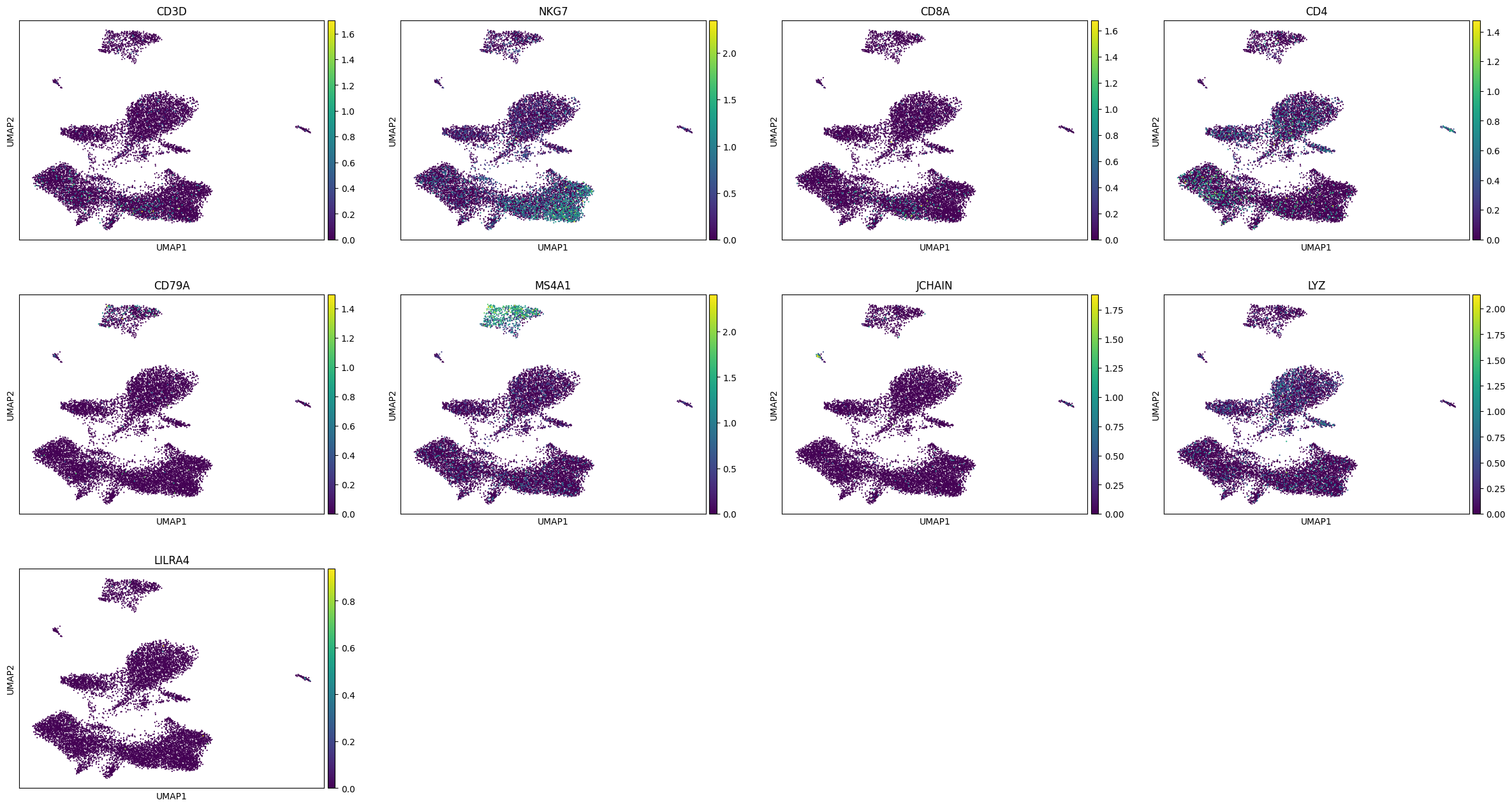

python

celltype = {
    '0': 'NK',
    '1': 'CD14+ Mono',
    '2': 'CD4+ T',
    '3': 'FCGR3A+ Mono',
    '4': 'B',
    '5': 'CD14+ Mono',
    '6': 'CD8+ T',
    '7': 'pDC',
    '8': 'Plasma'
}

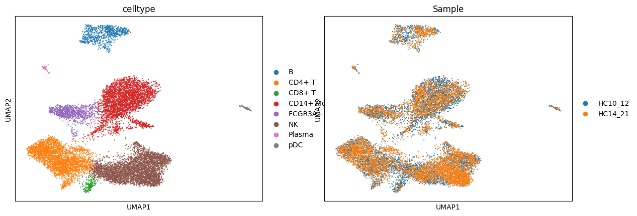
adata_rna.obs['celltype'] = adata_rna.obs['leiden'].map(celltype)

python

sc.pl.umap(adata_rna, color = ['celltype', 'Sample'])

output

/PROJ2/FLOAT/jinwen/apps/miniconda3/envs/allcools/lib/python3.8/site-packages/scanpy/plotting/_tools/scatterplots.py:394: UserWarning: No data for colormapping provided via 'c'. Parameters 'cmap' will be ignored
cax = scatter(
/PROJ2/FLOAT/jinwen/apps/miniconda3/envs/allcools/lib/python3.8/site-packages/scanpy/plotting/_tools/scatterplots.py:394: UserWarning: No data for colormapping provided via 'c'. Parameters 'cmap' will be ignored
cax = scatter(

Single-cell Methylation Sequencing Data Analysis Pipeline

Data Preprocessing

Matrix Binarization

Sets 95% threshold for data binarization:

Above threshold: Marked as hypermethylated state
Below threshold: Marked as hypomethylated state
Purpose: To highlight significant epigenetic differences

Region Filtering

Intelligently filters genomic regions, retaining:

Highly variable methylation regions
Informative epigenetic markers

Feature Extraction and Dimensionality Reduction

LSI (Latent Semantic Indexing) Analysis

Uses ARPACK algorithm for linear dimensionality reduction, extracting:

Principal components of genomic methylation patterns
Epigenetic similarity between cells
Methylation features in low-dimensional space

Batch Effect Correction

Harmony Ensemble Learning

Input: LSI reduction results + Sample metadata
Batch Variable: Sample source (SAMple)
Random Seed: 0 (Ensures reproducibility)
Max Iterations: 20 (Balances speed and accuracy)
Output: Corrected epigenetic space

Correction Effect:

Cleans technical variation between samples
Enhances fidelity of biological signals

Cell Atlas Construction

Neighbor Graph Construction

Based on the corrected feature space, builds a 30-nearest neighbor network of cells to quantify epigenetic similarity.

Clustering Analysis

Uses Leiden algorithm for cell population identification:

Clustering basis: Similarity in hypomethylation features
Output: Epigenetically defined cell clusters

python

# MET data integration
# Read Methylation mcds
obj_met_list = {}
mcds_paths = {}
for i in samples:
    mcds_path = os.path.join(f'{i}', f'{i}_methy','step3','allcools_generate_datasets', f'{i}.mcds')
    
    mcds_paths[i] = mcds_path
    mcds = MCDS.open(mcds_path, obs_dim = 'cell', var_dim = var_dim)
    adata = mcds.get_score_adata(mc_type=mc_type, quant_type=quant_type, sparse = True)
    obj_met_list[i] = adata

adata_met = obj_met_list[samples[0]].concatenate([obj_met_list[i] for i in samples[1:] ])



adata_met.layers['raw'] = adata_met.X.copy()
adata_met.obs['Sample'] = adata_met.obs['batch'].map(
    {f'{index}': value for index, value in enumerate(samples)}
)
binarize_matrix(adata_met, cutoff=0.95)
filter_regions(adata_met)

lsi(adata_met, algorithm='arpack', obsm='X_lsi')
significant_pc_test(adata_met, p_cutoff=0.1, obsm='X_lsi', update=True)

ho = run_harmony(adata_met.obsm['X_lsi'],
                 meta_data=adata_met.obs,
                 vars_use='Sample',
                 random_state=0,
                 max_iter_harmony=20)
adata_met.obsm['X_lsi_harmony'] = ho.Z_corr.T
reduc_use = 'X_lsi_harmony'

sc.pp.neighbors(adata_met,use_rep = reduc_use, n_neighbors=30)
sc.tl.umap(adata_met)
sc.tl.tsne(adata_met,use_rep=reduc_use)
sc.tl.leiden(adata_met, resolution=0.5)
#adata_met.write_h5ad('adata_met.h5ad')

output

Loading chunk 0-4269/4269
Loading chunk 0-4254/4254

/PROJ2/FLOAT/jinwen/apps/miniconda3/envs/allcools/lib/python3.8/site-packages/anndata/_core/anndata.py:1763: FutureWarning: The AnnData.concatenate method is deprecated in favour of the anndata.concat function. Please use anndata.concat instead.

See the tutorial for concat at: https://anndata.readthedocs.io/en/latest/concatenation.html
warnings.warn(

87948 regions remained.

2025-12-19 09:43:25,691 - harmonypy - INFO - Computing initial centroids with sklearn.KMeans...n

9 components passed P cutoff of 0.1.
Changing adata.obsm['X_pca'] from shape (8523, 100) to (8523, 9)

2025-12-19 09:43:27,280 - harmonypy - INFO - sklearn.KMeans initialization complete.
2025-12-19 09:43:27,315 - harmonypy - INFO - Iteration 1 of 20
2025-12-19 09:43:29,489 - harmonypy - INFO - Iteration 2 of 20
2025-12-19 09:43:31,702 - harmonypy - INFO - Iteration 3 of 20
2025-12-19 09:43:33,883 - harmonypy - INFO - Iteration 4 of 20
2025-12-19 09:43:36,109 - harmonypy - INFO - Iteration 5 of 20
2025-12-19 09:43:38,285 - harmonypy - INFO - Iteration 6 of 20
2025-12-19 09:43:40,491 - harmonypy - INFO - Iteration 7 of 20
2025-12-19 09:43:42,737 - harmonypy - INFO - Iteration 8 of 20
2025-12-19 09:43:44,954 - harmonypy - INFO - Iteration 9 of 20
2025-12-19 09:43:46,153 - harmonypy - INFO - Iteration 10 of 20
2025-12-19 09:43:47,429 - harmonypy - INFO - Iteration 11 of 20
2025-12-19 09:43:48,468 - harmonypy - INFO - Iteration 12 of 20
2025-12-19 09:43:49,388 - harmonypy - INFO - Iteration 13 of 20
2025-12-19 09:43:50,300 - harmonypy - INFO - Iteration 14 of 20
2025-12-19 09:43:51,118 - harmonypy - INFO - Iteration 15 of 20
2025-12-19 09:43:52,079 - harmonypy - INFO - Converged after 15 iterations

python

rna_meta = adata_rna.obs
rna_meta["gex_cb"] = rna_meta.index
rna_meta["gex_cb"] =[re.sub('-.*','', b) for b in rna_meta["gex_cb"] ]
rna_meta = rna_meta.merge(gex_mc_bc_map)
rna_meta["m_cb"] = rna_meta["m_cb"].astype(str) + "-" + rna_meta["batch"].astype(str)
rna_meta.index = rna_meta["m_cb"]
rna_meta = rna_meta.loc[adata_met.obs.index,]
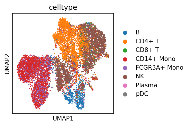
adata_met.obs["celltype"] = rna_meta["celltype"]
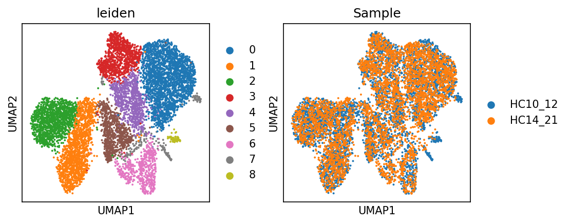
adata_met.obs["celltype"] = adata_met.obs["celltype"].astype('category')

python

plt.rcParams['figure.dpi'] = 150
plt.rcParams['figure.figsize'] = (3,3)
sc.pl.umap(adata_met, color = ['leiden', 'Sample'])

output

python

sc.pl.umap(adata_met, color = ['celltype'])

output

Cell Composition Proportions

Shows relative abundance of cell types in different samples. Stacked bar charts intuitively reflect inter-sample heterogeneity in cell composition.

Sample-Cell Type Proportion Distribution Plot

This plot shows the proportion of different methylation cell types in each sample.

X-axis: Represents different samples (SAMple).
Y-axis: Represents cell proportion (Proportion, 0-1.0).
Color: Different colored blocks represent different methylation cell types.

python

def plot_bar_fraction_data(adata, x_key, y_key):
    df = adata_met.obs[[x_key, y_key]].copy()
    df[y_key] = df[y_key].astype('category')
    df[x_key] = df[x_key].astype('category')
    
    counts = df.groupby([x_key, y_key]).size().reset_index(name='count')
    totals = counts.groupby(x_key)['count'].transform('sum')
    counts['prop'] = counts['count'] / totals
    
    prop_pivot = counts.pivot(index=x_key, columns=y_key, values='prop').fillna(0)
    
    clusters = list(prop_pivot.columns)
    if f'{y_key}_colors' in adata_met.uns.keys():
        palette = adata.uns['celltype_colors']
    palette = sc.pl.palettes.default_20
    color_map = {c: palette[i % len(palette)] for i, c in enumerate(clusters)}
    bar_colors = [color_map[c] for c in clusters]

    return prop_pivot, bar_colors


# Calculate proportion of each cluster per sample and plot stacked bar chart
y_key = 'celltype'
prop_pivot, bar_colors = plot_bar_fraction_data(adata_met, x_key = "Sample", y_key = y_key)
plt.rcParams['figure.dpi'] = 150
plt.rcParams['figure.figsize'] = (3,3)
fig, ax = plt.subplots()
prop_pivot.plot(kind='bar', stacked=True, color=bar_colors, ax=ax)
ax.set_ylabel('Proportion')
ax.set_xlabel("Sample")
ax.legend(title=y_key, bbox_to_anchor=(1, 1), loc='upper left', frameon=False, fontsize=7, markerscale=0.5, handlelength=1.0, handletextpad=0.4, borderaxespad=0.4)
plt.tight_layout()

#prop_pivot.to_csv(f'{sample_col}_{y_key}_frac.csv')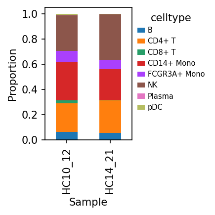

Spatial Distribution Visualization of QC Metrics

QC Metrics Distribution Analysis: UMAP Visualization

Visualization Purpose

By visualizing key QC metrics in UMAP space, we can intuitively assess data quality distribution patterns across cell populations, identify potential technical bias regions, and verify reliability of cell subpopulation partitioning.

total_cpg_number | Total CpG Sites

Interpretation: Color gradient from dark blue to bright yellow reflects the total number of methylation sites captured per cell.

Bright Yellow Regions: Information-rich, comprehensive methylation landscape
Dark Blue Regions: Sparse data, interpret biological significance with caution
Abnormal Patterns: Consistently low values in specific cell clusters may suggest technical issues

reads_counts | Sequencing Depth

Interpretation: Shows the number of unique aligned sequences per cell.

Depth and Accuracy: Sufficient sequencing depth guarantees methylation quantification accuracy
QC Standard: Systematically low-depth regions may require technical filtering

genome_cov | Genome Coverage (0-1)

Interpretation: Quantifies the proportion of genomic regions covered by sequencing data.

Comprehensiveness: High coverage represents a more complete epigenetic profile
Technical Validation: Abnormally low coverage may point to cell lysis or amplification issues

CpG% | CpG Methylation Rate (0-100%)

Interpretation: Shows overall methylation level of CpG sites.

Functional Association: Usually associated with gene silencing and chromatin state
Cell State: Cells in different differentiation or functional states may show characteristic patterns
Quality Relation: Extreme high/low values may reflect technical anomalies rather than biological differences

CH% | CH Non-CpG Methylation Rate (0-100%)

Interpretation: Reveals modification levels of non-canonical methylation sites.

Biological Specialization: Has regulatory significance in specific types like neurons, stem cells
Signal Identification: Complementary to CpG% patterns, providing a more comprehensive epigenetic view
Baseline Reference: Usually maintained at low levels in mammals; abnormally high values need careful validation

python

def compute_cg_ch_level(df):
    # comput cpg methylation levels and ch methylation levels
    cg_cov_col = [i for i in df.columns[df.columns.str.startswith('CG')].to_list() if i.endswith('_cov')]
    cg_mc_col = [i for i in df.columns[df.columns.str.startswith('CG')].to_list() if i.endswith('_mc')]
    ch_cov_col = [i for i in df.columns[df.columns.str.contains('^(CT|CC|CA)')].to_list() if i.endswith('_cov')]
    ch_mc_col = [i for i in df.columns[df.columns.str.contains('^(CT|CC|CA)')].to_list() if i.endswith('_mc')]
    
    df['CpG_cov'] = df[cg_cov_col].sum(axis=1)
    df['CpG_mc'] = df[cg_mc_col].sum(axis=1)
    df['CpG%'] = round(df['CpG_mc'] * 100 / df['CpG_cov'], 2)
    
    df['CH_cov'] = df[ch_cov_col].sum(axis=1)
    df['CH_mc'] = df[ch_mc_col].sum(axis=1)
    df['CH%'] = round(df['CH_mc'] * 100 / df['CH_cov'], 2)

    return df


suffix_map = {f'{value}': index for index, value in enumerate(samples)}
meta_list = list()
keep_col = ['barcode', 'total_cpg_number', 'genome_cov', 'reads_counts', 'CpG%', 'CH%']

for i in samples: 

    s_cells_meta = pd.read_csv(os.path.join(f'{i}', f'{i}_methy', 'step3', 'split_bams','merged', f'{i}_cells.csv'), header = 0)
    s_cells_meta['barcode'] = [b.replace('_allc.gz','') for b in s_cells_meta['cell_barcode']]
    s_reads_counts = pd.read_csv(os.path.join(f'{i}', f'{i}_methy', 'step3', 'split_bams','merged', 'filtered_barcode_reads_counts.csv'), header = 0)
    s_merged_df = s_cells_meta.merge(s_reads_counts, how = 'inner', left_on = 'barcode', right_on = 'barcode')
    s_merged_df = compute_cg_ch_level(s_merged_df)
    s_merged_df = s_merged_df[keep_col]
    if len(samples) > 1:
        s_merged_df['barcode'] = [f'{b}-{suffix_map[i]}'for b in s_merged_df['barcode']]
    meta_list.append(s_merged_df)
adata_met.obs = adata_met.obs.merge(
    pd.concat(meta_list).set_index('barcode'), 
    how = 'left', 
    left_index=True, 
    right_index = True)

output

/tmp/ipykernel_143/2478518388.py:5: UserWarning: This pattern is interpreted as a regular expression, and has match groups. To actually get the groups, use str.extract.
ch_cov_col = [i for i in df.columns[df.columns.str.contains('^(CT|CC|CA)')].to_list() if i.endswith('_cov')]
/tmp/ipykernel_143/2478518388.py:6: UserWarning: This pattern is interpreted as a regular expression, and has match groups. To actually get the groups, use str.extract.
ch_mc_col = [i for i in df.columns[df.columns.str.contains('^(CT|CC|CA)')].to_list() if i.endswith('_mc')]
/tmp/ipykernel_143/2478518388.py:5: UserWarning: This pattern is interpreted as a regular expression, and has match groups. To actually get the groups, use str.extract.
ch_cov_col = [i for i in df.columns[df.columns.str.contains('^(CT|CC|CA)')].to_list() if i.endswith('_cov')]
/tmp/ipykernel_143/2478518388.py:6: UserWarning: This pattern is interpreted as a regular expression, and has match groups. To actually get the groups, use str.extract.
ch_mc_col = [i for i in df.columns[df.columns.str.contains('^(CT|CC|CA)')].to_list() if i.endswith('_mc')]

python

plt.rcParams['figure.dpi'] = 150
plt.rcParams['figure.figsize'] = (3,3)
sc.pl.umap(adata_met, color = ['total_cpg_number','reads_counts','genome_cov'], cmap = 'inferno')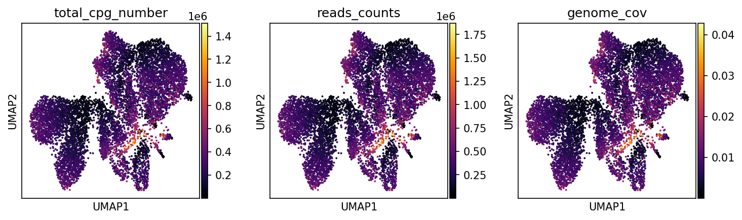

python

plt.rcParams['figure.dpi'] = 150
plt.rcParams['figure.figsize'] = (3,3)
sc.pl.umap(adata_met, color = ['CpG%','CH%'], cmap = 'inferno')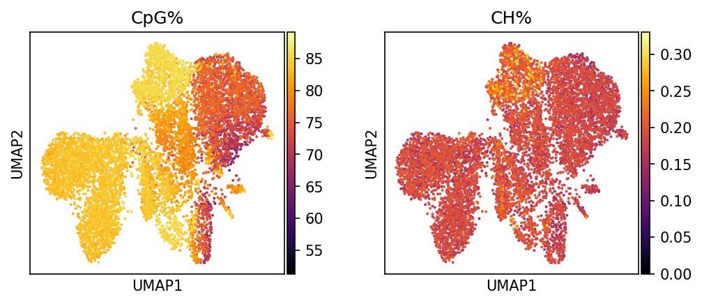

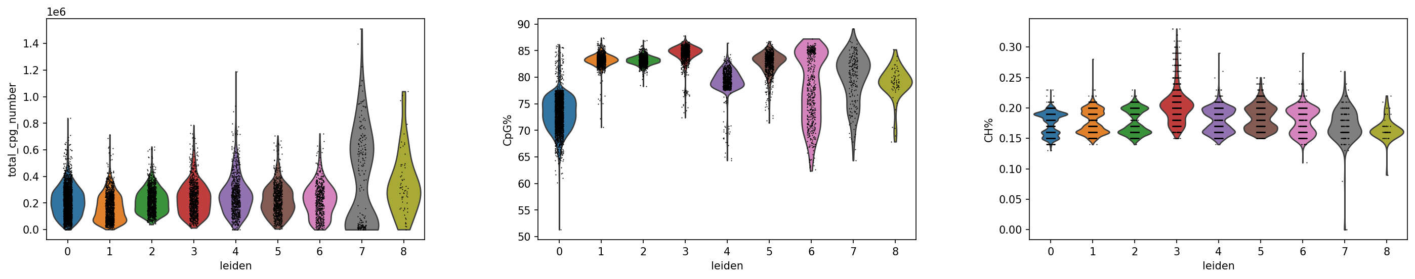
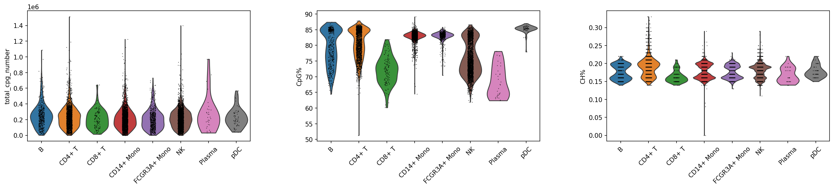
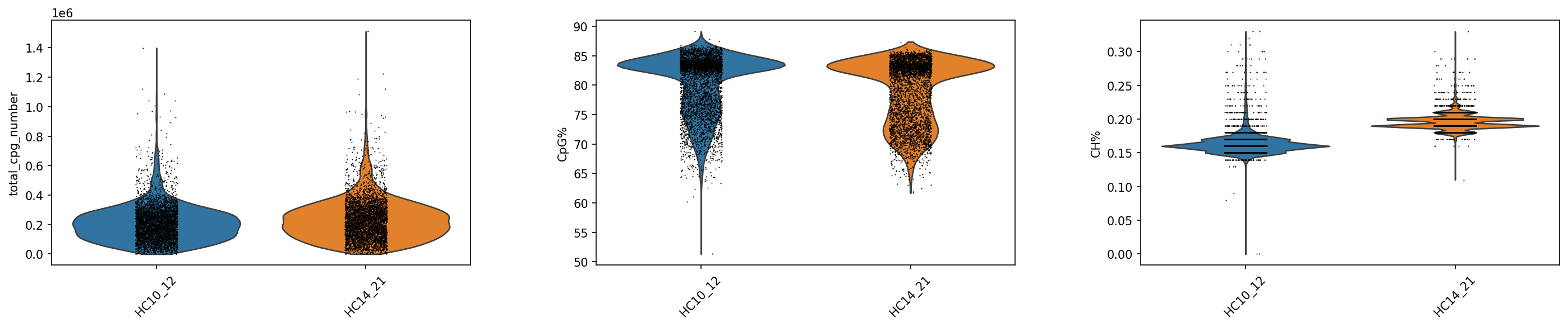
QC Metrics Distribution Analysis: Violin Plot Visualization

Visualization Purpose

Using Violin Plots to intuitively display distribution characteristics of key QC metrics across different cell groups, assessing data quality uniformity, identifying potential batch effects or technical biases, and ensuring reliability of subsequent biological findings.

CpG Site Count Distribution

Ideal Pattern: Similar distribution across clusters, medians close
Abnormal Warning: Significantly lower site counts in specific clusters
Biological Significance: Reflects cell capture efficiency and DNA quality

CpG Methylation Rate Distribution

Expected Range: Usually maintains a relatively stable baseline level in mammalian cells
Inter-cluster Differences: Different cell types may show characteristic methylation levels
QC Standard: Abnormally low/high values may indicate technical issues

CH Methylation Rate Distribution

Baseline Characteristics: Usually far lower than CpG methylation rate
Biological Specificity: May be elevated in specific types like neurons, embryonic stem cells
Technical Differentiation: Need to distinguish real biological features from technical biases

python

plt.rcParams['figure.figsize'] = (6,4)
sc.pl.violin(adata_met, keys=['total_cpg_number', 'CpG%', 'CH%'], groupby='leiden')
#_ = sc.pl.violin(adata_met, keys=['total_cpg_number', 'CpG%', 'CH%'], groupby='leiden', save = '_leiden_cpg_ch.png', show = False)

output

/PROJ2/FLOAT/jinwen/apps/miniconda3/envs/allcools/lib/python3.8/site-packages/scanpy/plotting/_anndata.py:839: FutureWarning:

Passing \`palette\` without assigning \`hue\` is deprecated and will be removed in v0.14.0. Assign the \`x\` variable to \`hue\` and set \`legend=False\` for the same effect.

ax = sns.violinplot(
/PROJ2/FLOAT/jinwen/apps/miniconda3/envs/allcools/lib/python3.8/site-packages/scanpy/plotting/_anndata.py:839: FutureWarning:

The \`scale\` parameter has been renamed and will be removed in v0.15.0. Pass \`density_norm='width'\` for the same effect.
ax = sns.violinplot(
/PROJ2/FLOAT/jinwen/apps/miniconda3/envs/allcools/lib/python3.8/site-packages/scanpy/plotting/_anndata.py:839: FutureWarning:

Passing \`palette\` without assigning \`hue\` is deprecated and will be removed in v0.14.0. Assign the \`x\` variable to \`hue\` and set \`legend=False\` for the same effect.

ax = sns.violinplot(
/PROJ2/FLOAT/jinwen/apps/miniconda3/envs/allcools/lib/python3.8/site-packages/scanpy/plotting/_anndata.py:839: FutureWarning:

The \`scale\` parameter has been renamed and will be removed in v0.15.0. Pass \`density_norm='width'\` for the same effect.
ax = sns.violinplot(
/PROJ2/FLOAT/jinwen/apps/miniconda3/envs/allcools/lib/python3.8/site-packages/scanpy/plotting/_anndata.py:839: FutureWarning:

Passing \`palette\` without assigning \`hue\` is deprecated and will be removed in v0.14.0. Assign the \`x\` variable to \`hue\` and set \`legend=False\` for the same effect.

ax = sns.violinplot(
/PROJ2/FLOAT/jinwen/apps/miniconda3/envs/allcools/lib/python3.8/site-packages/scanpy/plotting/_anndata.py:839: FutureWarning:

The \`scale\` parameter has been renamed and will be removed in v0.15.0. Pass \`density_norm='width'\` for the same effect.
ax = sns.violinplot(

python

plt.rcParams['figure.figsize'] = (6,4)
sc.pl.violin(adata_met, keys=['total_cpg_number', 'CpG%', 'CH%'], groupby="celltype",rotation = 45)
#_ = sc.pl.violin(adata_met, keys=['total_cpg_number', 'CpG%', 'CH%'], groupby=anno_col, save = f'_{anno_col}_cpg_ch.png', rotation = 45,show = False)

output

python

plt.rcParams['figure.figsize'] = (6,4)
sc.pl.violin(adata_met, keys=['total_cpg_number', 'CpG%', 'CH%'], groupby="Sample",rotation = 45)
#_ = sc.pl.violin(adata_met, keys=['total_cpg_number', 'CpG%', 'CH%'], groupby=sample_col, save = f'_{sample_col}_cpg_ch.png',rotation = 45, show = False)

output

python

adata_met.write_h5ad('adata_met.h5ad')

Single-cell Methylation + RNA Dual-omics Multi-sample Integration Analysis Pipeline (ALLCools) ​

Load Python Analysis Packages ​

Single-cell RNA Sequencing Data Multi-sample Integration Analysis Pipeline ​

Data Preprocessing Pipeline ​

Normalization and Transformation ​

Feature Gene Selection ​

Batch Effect Correction ​

Application of Harmony Algorithm ​

Cell Atlas Construction ​

Neighborhood Relationship Calculation ​

Clustering Analysis ​

Visualization ​

RNA Single-modality Cell Annotation ​

Single-cell Methylation Sequencing Data Analysis Pipeline ​

Data Preprocessing ​

Matrix Binarization ​

Region Filtering ​

Feature Extraction and Dimensionality Reduction ​

LSI (Latent Semantic Indexing) Analysis ​

Batch Effect Correction ​

Harmony Ensemble Learning ​

Cell Atlas Construction ​

Neighbor Graph Construction ​

Clustering Analysis ​

Cell Composition Proportions ​

Spatial Distribution Visualization of QC Metrics ​

QC Metrics Distribution Analysis: UMAP Visualization ​

Visualization Purpose ​

total_cpg_number | Total CpG Sites ​

reads_counts | Sequencing Depth ​

genome_cov | Genome Coverage (0-1) ​

CpG% | CpG Methylation Rate (0-100%) ​

CH% | CH Non-CpG Methylation Rate (0-100%) ​

QC Metrics Distribution Analysis: Violin Plot Visualization ​

Visualization Purpose ​

CpG Site Count Distribution ​

CpG Methylation Rate Distribution ​

CH Methylation Rate Distribution ​

Single-cell Methylation + RNA Dual-omics Multi-sample Integration Analysis Pipeline (ALLCools)

Load Python Analysis Packages

Single-cell RNA Sequencing Data Multi-sample Integration Analysis Pipeline

Data Preprocessing Pipeline

Normalization and Transformation

Feature Gene Selection

Batch Effect Correction

Application of Harmony Algorithm

Cell Atlas Construction

Neighborhood Relationship Calculation

Clustering Analysis

Visualization

RNA Single-modality Cell Annotation

Single-cell Methylation Sequencing Data Analysis Pipeline

Data Preprocessing

Matrix Binarization

Region Filtering

Feature Extraction and Dimensionality Reduction

LSI (Latent Semantic Indexing) Analysis

Batch Effect Correction

Harmony Ensemble Learning

Cell Atlas Construction

Neighbor Graph Construction

Clustering Analysis

Cell Composition Proportions

Spatial Distribution Visualization of QC Metrics

QC Metrics Distribution Analysis: UMAP Visualization

Visualization Purpose

total_cpg_number | Total CpG Sites

reads_counts | Sequencing Depth

genome_cov | Genome Coverage (0-1)

CpG% | CpG Methylation Rate (0-100%)

CH% | CH Non-CpG Methylation Rate (0-100%)

QC Metrics Distribution Analysis: Violin Plot Visualization

Visualization Purpose

CpG Site Count Distribution

CpG Methylation Rate Distribution

CH Methylation Rate Distribution