Single-cell Gene Expression Dynamics: Pseudotime Gene Expression Curve Fitting

Author: SeekGene

Time: 3 min

Words: 527 words

Updated: 2026-02-27

Reads: 0 times

3' scRNA-seq 5' + Immune Profiling FFPE scRNA-seq Notebooks Pseudotime Analysis Spatial-seq scATAC + RNA-seq scFAST-seq scMethyl + RNA-seq

Environment Setup

# Load required R packages
library(monocle)
library(Seurat)
library(dplyr)
library(tidyverse)
library(ggplot2)
library(ggsci)

Data Loading

# Read data
gbm_cds <- readRDS("data/AY1740561864613/advanced_analysis/58047/output/monocle2/monocle_final.rds") ### Monocle2 analysis results
rep <- as.data.frame(pData(gbm_cds)) # Read phenotype information
gene_all <- row.names(gbm_cds@assayData$exprs)  # Get all genes in gbm_cds

Data Preprocessing

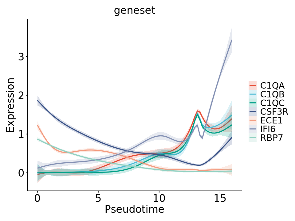
gene_ad <- c("RBP7","ECE1","C1QA","C1QC","C1QB","IFI6","CSF3R")  # Define genes to display (max 10)

# Intersect gene_ad with genes_all
gene_se <- vector()
for(i in gene_ad){
    if(i %in% gene_all){
        gene_se <- c(gene_se,i)
    }
}

# Extract gene expression levels
for(i in gene_se){
    gene_in <- names(pData(gbm_cds))
    if (i %in% gene_in){
        next
    }else{
        tmp <- gbm_cds@assayData$exprs[i,] %>% as.data.frame
        names(tmp) <- i
        tmp <- tmp %>% mutate(barcode=rownames(tmp))
        pData(gbm_cds) <- pData(gbm_cds) %>% inner_join(tmp,by="barcode")
        rownames(pData(gbm_cds)) <- pData(gbm_cds)$barcode
    }
}

# Merge expression data with pseudotime info
data_plot <- pData(gbm_cds) %>% select(Pseudotime,all_of(gene_se)) %>% 
pivot_longer(cols = -Pseudotime,names_to = "Gene",values_to = "Expression")

Pseudotime Curve Plotting

# Set plot output dimensions (for interactive environments like Jupyter)
# repr.plot.height: Plot height 6 inches
# repr.plot.width: Plot width 8 inches
options(repr.plot.height=6, repr.plot.width=8)

# Create ggplot object
ggplot(data = data_plot, mapping = aes(x = Pseudotime, 
                                      y = Expression, 
                                      color = Gene,   # Color by gene
                                      fill = Gene)) +  # Fill color by gene
        # Use Nature Publishing Group color scheme (npg)
        ggsci::scale_color_npg(name = "") +  # Discrete color scale
        ggsci::scale_fill_npg(name = "") +   # Discrete fill color scale
        
        # Add GAM smoothing curve (confidence interval band)
        # method: Use Generalized Additive Model
        # formula: Cubic spline basis function
        # alpha: Confidence interval transparency (0-1)
        # size: Curve line width
        geom_smooth(method = "gam", 
                   formula = y ~ s(x, bs = "cs"), 
                   alpha = 0.2, 
                   size = 1) +
        
        # Apply cowplot theme (concise scientific style)
        cowplot::theme_cowplot() +
        
        # Customize theme details
        theme(
            axis.text.x = element_text(size = 20),  # X-axis tick label size
            axis.text.y = element_text(size = 20),  # Y-axis tick label size
            text = element_text(size = 20, family = "ArialMT"),  # Global font settings
            plot.margin = unit(c(1, 1, 1, 1), "char"),  # Plot margins (character units)
            plot.title = element_text(
                hjust = 0.5,         # Center title
                size = 20,           # Title font size
                family = "ArialMT",  # Font family
                face = "plain"       # No bold
            ),
            axis.line = element_line(
                linetype = 1,        # Solid line type
                color = "black",     # Axis line color
                linewidth = 0.6      # Axis line width
            ),
            axis.ticks = element_line(
                linetype = 1,        # Tick line type
                color = "black",     # Tick line color
                linewidth = 0.6      # Tick line width
            )
            # legend.position = "none"  # Hide legend (currently commented out)
        ) +
        
        # Axis Label Settings
        ylab("Expression") +    # Y-axis label (Gene Expression) 
        xlab("Pseudotime") +     # X-axis label (Pseudotime Analysis Result)
        ggtitle("geneset")      # Main Title
        
        # Save Output (Publication Quality)
        # filename: Output filename
        # width: PDF width 9 inches (approx 22.86cm)
        # height: PDF height 8 inches (approx 20.32cm)
        ggsave("expression.pdf", width = 9, height = 8)