单细胞基因表达动态解析：拟时序基因表达量曲线拟合

作者: SeekGene

时长: 4 分钟

字数: 727 字

更新: 2026-02-27

阅读: 0 次

3' 转录组 5' + 免疫组库 ATAC + RNA 双组学 FFPE 单细胞转录组 Notebooks 全序列转录组 拟时序分析 甲基化 + RNA 双组学 空间转录组

环境配置

# 加载脚本运行依赖的R包
library(monocle)
library(Seurat)
library(dplyr)
library(tidyverse)
library(ggplot2)
library(ggsci)

数据读取

#读取数据
gbm_cds <- readRDS("data/AY1740561864613/advanced_analysis/58047/output/monocle2/monocle_final.rds") ### monocle2分析结果
rep <- as.data.frame(pData(gbm_cds)) # 读取表型信息
gene_all <- row.names(gbm_cds@assayData$exprs)  #获取gbm_cds中全部基因

数据预处理

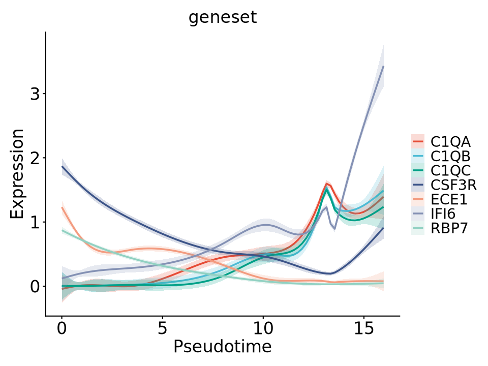
gene_ad <- c("RBP7","ECE1","C1QA","C1QC","C1QB","IFI6","CSF3R")  #定义图中要展示的基因，最多展示10个基因

# gene_ad 与 genes_all 取交集
gene_se <- vector()
for(i in gene_ad){
    if(i %in% gene_all){
        gene_se <- c(gene_se,i)
    }
}

# 提取基因表达量
for(i in gene_se){
    gene_in <- names(pData(gbm_cds))
    if (i %in% gene_in){
        next
    }else{
        tmp <- gbm_cds@assayData$exprs[i,] %>% as.data.frame
        names(tmp) <- i
        tmp <- tmp %>% mutate(barcode=rownames(tmp))
        pData(gbm_cds) <- pData(gbm_cds) %>% inner_join(tmp,by="barcode")
        rownames(pData(gbm_cds)) <- pData(gbm_cds)$barcode
    }
}

# 合并表达量信息和拟时序信息
data_plot <- pData(gbm_cds) %>% select(Pseudotime,all_of(gene_se)) %>% 
pivot_longer(cols = -Pseudotime,names_to = "Gene",values_to = "Expression")

拟时序曲线绘制

# 设置图形输出尺寸（适用于Jupyter等交互环境）
# repr.plot.height: 图形高度6英寸
# repr.plot.width: 图形宽度8英寸
options(repr.plot.height=6, repr.plot.width=8)

# 创建ggplot对象
ggplot(data = data_plot, mapping = aes(x = Pseudotime, 
                                      y = Expression, 
                                      color = Gene,   # 按基因分组颜色
                                      fill = Gene)) +  # 按基因分组填充色
        # 使用Nature出版集团配色方案（npg）
        ggsci::scale_color_npg(name = "") +  # 离散型颜色标尺
        ggsci::scale_fill_npg(name = "") +   # 离散型填充色标尺
        
        # 添加GAM平滑曲线（置信区间带）
        # method: 使用广义加性模型
        # formula: 三次平滑样条基函数（cubic spline basis）
        # alpha: 置信区间透明度（0-1）
        # size: 曲线线宽
        geom_smooth(method = "gam", 
                   formula = y ~ s(x, bs = "cs"), 
                   alpha = 0.2, 
                   size = 1) +
        
        # 应用cowplot主题（简洁科研风格）
        cowplot::theme_cowplot() +
        
        # 自定义主题细节
        theme(
            axis.text.x = element_text(size = 20),  # X轴刻度标签字号
            axis.text.y = element_text(size = 20),  # Y轴刻度标签字号
            text = element_text(size = 20, family = "ArialMT"),  # 全局字体设置
            plot.margin = unit(c(1, 1, 1, 1), "char"),  # 图形边距（字符单位）
            plot.title = element_text(
                hjust = 0.5,         # 标题居中
                size = 20,           # 标题字号
                family = "ArialMT",  # 字体类型
                face = "plain"       # 无加粗
            ),
            axis.line = element_line(
                linetype = 1,        # 实线类型
                color = "black",     # 轴线颜色
                linewidth = 0.6      # 轴线宽度
            ),
            axis.ticks = element_line(
                linetype = 1,        # 刻度线类型
                color = "black",     # 刻度线颜色
                linewidth = 0.6      # 刻度线宽度
            )
            # legend.position = "none"  # 取消图例显示（当前注释状态）
        ) +
        
        # 坐标轴标签设置
        ylab("Expression") +    # Y轴标签（基因表达量） 
        xlab("Pseudotime") +     # X轴标签（拟时序分析结果）
        ggtitle("geneset")      # 主标题
        
        # 保存输出（出版级分辨率）
        # filename: 输出文件名
        # width: PDF宽度9英寸（约22.86cm）
        # height: PDF高度8英寸（约20.32cm）
        ggsave("expression.pdf", width = 9, height = 8)