Single-cell Fine Resolution: Cell Clustering Strategy Based on LncRNA Expression Features
This article explores a supplementary strategy for cell clustering in single-cell RNA sequencing analysis using long non-coding RNAs (LncRNAs) in addition to traditional highly variable genes. LncRNA expression has higher cell state specificity, helping to identify fine subpopulations difficult to distinguish by traditional methods; meanwhile, its expression can be directly linked to epigenetic regulatory activity of cells, providing functional interpretation for clustering. This method helps discover novel cell states or biomarkers when traditional clustering resolution is insufficient.
For example, study [1] used this method to find new cell subpopulations and key LncRNA markers; another study [2] also distinguished cell subpopulations with different characteristics through LncRNA.
Here we recommend a two-step clustering method: first determine major cell types using classic highly variable genes, then use LncRNA for secondary clustering within target subpopulations. This strategy can exclude background interference between major types and focus on heterogeneity within the same lineage, thereby more accurately resolving cell functional states, developmental trajectories, or pathological transitions.
Here we use SeekGene public data as an example. LncRNA clustering applies to various data types such as DD3 transcriptome/DD full-sequence transcriptome/DD5 transcriptome. Many LncRNA genes have poly-A tails, and data obtained by conventional single-cell RNA capture methods can satisfy clustering analysis.
options(repr.plot.width = 6, repr.plot.height = 6)Code Example
Load Required R Packages
library(Seurat)
library(harmony)
library(plotly)
library(ggplot2)
library(dplyr)
library(tidyverse)
library(RColorBrewer)
library(ggalluvial)
Read RDS Data
obj=readRDS("../../../data/WorkflowID/input.rds")
meta=read.delim("../../../data/WorkflowID/meta.tsv")

rownames(meta)=meta$barcode
obj=AddMetaData(obj,metadata = meta)
Calculate Variable Features for All Genes
obj <- FindVariableFeatures(obj, nfeatures = dim(obj)[1], verbose = FALSE)
hvg_all_features <- VariableFeatures(obj)
head(hvg_all_features)“The \`slot\` argument of \`GetAssayData()\` is deprecated as of SeuratObject 5.0.0.
ℹ Please use the \`layer\` argument instead.
ℹ The deprecated feature was likely used in the Seurat package.
Please report the issue at
- 'IGHV4-59'
- 'IGKV1D-39'
- 'IGHV4-61'
- 'IGHV3-30'
- 'PTGDS'
- 'IGKV4-1'
Read Gene Types
gene_biotype = read.csv("../GRCh38_gene_biotype.csv")
## Human GRCh38 genome can directly read the following data
#gene_biotype = read.csv("https://seekgene-public.oss-cn-beijing.aliyuncs.com/software/FAST/GRCh38_gene_biotype.csv")
## Mouse mm10 genome can directly read the following data
#gene_biotype = read.csv("https://seekgene-public.oss-cn-beijing.aliyuncs.com/software/FAST/mm10_gene_biotype.csv")
head(gene_biotype)
dim(gene_biotype)| gene_id | gene_type | gene_name | |
|---|---|---|---|
| <chr> | <chr> | <chr> | |
| 1 | ENSG00000243485 | lncRNA | MIR1302-2HG |
| 2 | ENSG00000237613 | lncRNA | FAM138A |
| 3 | ENSG00000186092 | protein_coding | OR4F5 |
| 4 | ENSG00000238009 | lncRNA | AL627309.1 |
| 5 | ENSG00000239945 | lncRNA | AL627309.3 |
| 6 | ENSG00000239906 | lncRNA | AL627309.2 |
- 36601
- 3
## Filter genes present only in rds and sort by hvg_all_features
all_genes=rownames(obj)
gene_biotype <- gene_biotype %>% filter(gene_name %in% hvg_all_features)
gene_biotype <- gene_biotype[match(hvg_all_features, gene_biotype$gene_name, nomatch = 0), ]
head(gene_biotype)| gene_id | gene_type | gene_name | |
|---|---|---|---|
| <chr> | <chr> | <chr> | |
| 13345 | ENSG00000224373 | IG_V_gene | IGHV4-59 |
| 2547 | ENSG00000251546 | IG_V_gene | IGKV1D-39 |
| 13346 | ENSG00000211970 | IG_V_gene | IGHV4-61 |
| 13331 | ENSG00000270550 | IG_V_gene | IGHV3-30 |
| 9429 | ENSG00000107317 | protein_coding | PTGDS |
| 2522 | ENSG00000211598 | IG_V_gene | IGKV4-1 |
Select Top 2000 LncRNA Genes, Protein-coding Genes, and All Genes Respectively
top_2000_coding_RNA <- gene_biotype %>%
    filter(gene_type == "protein_coding")  %>%
    select(gene_name) %>%
    top_n(2000) %>%
    pull()
top_2000_lnc_RNA <- gene_biotype %>%
    filter(gene_type == "lncRNA")  %>%
    select(gene_name) %>%
    top_n(2000) %>%
    pull()
top_2000_all <- gene_biotype %>%
    select(gene_name) %>%
    top_n(2000) %>%
pull()Selecting by gene_name
Selecting by gene_name
redu="harmony" # If rds has not removed batch effects, specify pca here
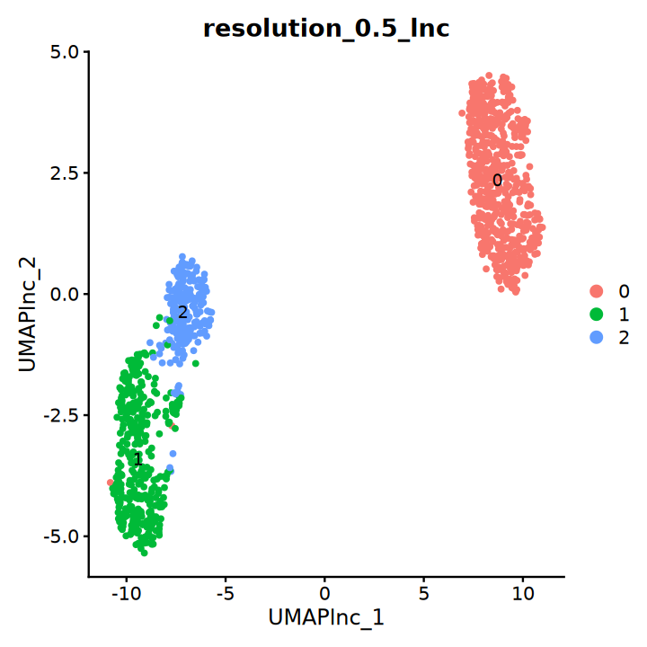
resolution_=0.5 # Set unified resolution to 0.5Dimensionality Reduction and Clustering Based on Top 2000 LncRNA Genes
VariableFeatures(obj) <- top_2000_lnc_RNA

obj <- RunUMAP(object = obj,
               assay = "RNA",
               reduction = redu,
               features  = top_2000_lnc_RNA,
               verbose = FALSE)
obj <- RunTSNE(object = obj,
               assay = "RNA",
               reduction = redu,
               features  = top_2000_lnc_RNA,
               verbose = FALSE)
obj <- FindNeighbors(object = obj,
                     assay = "RNA",
                     reduction = redu,
                     dims = NULL,
                     features  = top_2000_lnc_RNA,
                     verbose = FALSE)
obj <- FindClusters(object = obj,
                    resolution = 0.5,
                    cluster.name = "resolution_0.5_lnc",
                    verbose = FALSE)


embed <- Embeddings(obj, reduction = "umap")
obj[["UMAP_lnc"]] <- CreateDimReducObject(embeddings = embed, key = "UMAPlnc_", assay = DefaultAssay(obj))

embed <- Embeddings(obj, reduction = "tsne")
obj[["TSNE_lnc"]] <- CreateDimReducObject(embeddings = embed, key = "TSNElnc_", assay = DefaultAssay(obj))

DimPlot(obj, group.by = "resolution_0.5_lnc", label = T, reduction = "UMAP_lnc")“The default method for RunUMAP has changed from calling Python UMAP via reticulate to the R-native UWOT using the cosine metric
To use Python UMAP via reticulate, set umap.method to 'umap-learn' and metric to 'correlation'
This message will be shown once per session”
Dimensionality Reduction and Clustering Based on Top 2000 Coding Genes
VariableFeatures(obj) <- top_2000_coding_RNA

obj <- RunUMAP(object = obj,
               assay = "RNA",
               reduction = redu,
               features  = top_2000_coding_RNA,
               verbose = FALSE)
obj <- RunTSNE(object = obj,
               assay = "RNA",
               reduction = redu,
               features  = top_2000_coding_RNA,
               verbose = FALSE)
obj <- FindNeighbors(object = obj,
                     assay = "RNA",
                     reduction = redu,
                     dims = NULL,
                     features  = top_2000_coding_RNA,
                     verbose = FALSE)
obj <- FindClusters(object = obj,
                    resolution = 0.5,
                    cluster.name = "resolution_0.5_coding",
                    verbose = FALSE)


embed <- Embeddings(obj, reduction = "umap")
obj[["UMAP_coding"]] <- CreateDimReducObject(embeddings = embed, key = "UMAPcoding_", assay = DefaultAssay(obj))

embed <- Embeddings(obj, reduction = "tsne")
obj[["TSNE_coding"]] <- CreateDimReducObject(embeddings = embed, key = "TSNEcoding_", assay = DefaultAssay(obj))

DimPlot(obj, group.by = "resolution_0.5_coding", label = T, reduction = "UMAP_coding")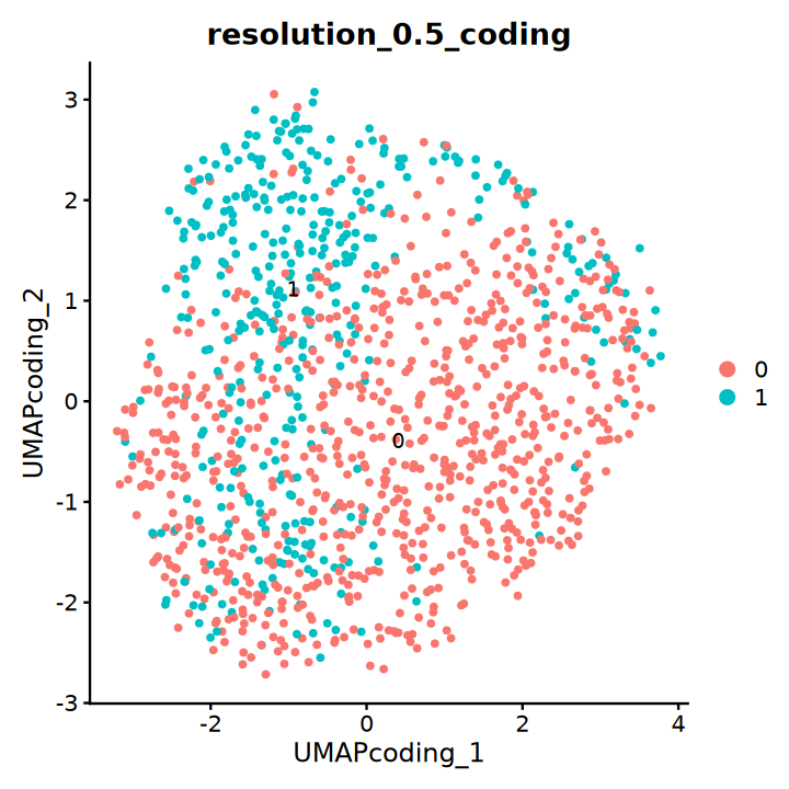
Dimensionality Reduction and Clustering Based on Top 2000 All Genes
VariableFeatures(obj) <- top_2000_all

obj <- RunUMAP(object = obj,
               assay = "RNA",
               reduction = redu,
               features  = top_2000_all,
               verbose = FALSE)
obj <- RunTSNE(object = obj,
               assay = "RNA",
               reduction = redu,
               features  = top_2000_all,
               verbose = FALSE)
obj <- FindNeighbors(object = obj,
                     assay = "RNA",
                     reduction = redu,
                     dims = NULL,
                     features  = top_2000_all,
                     verbose = FALSE)
obj <- FindClusters(object = obj,
                    resolution = 0.5,
                    cluster.name = "resolution_0.5_all",
                    verbose = FALSE)

embed <- Embeddings(obj, reduction = "umap")
obj[["UMAP_all"]] <- CreateDimReducObject(embeddings = embed, key = "UMAPall_", assay = DefaultAssay(obj))

embed <- Embeddings(obj, reduction = "tsne")
obj[["TSNE_all"]] <- CreateDimReducObject(embeddings = embed, key = "TSNEall_", assay = DefaultAssay(obj))

DimPlot(obj, group.by = "resolution_0.5_all", label = T, reduction = "UMAP_all")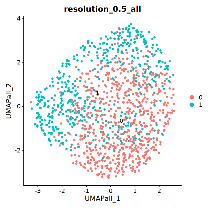
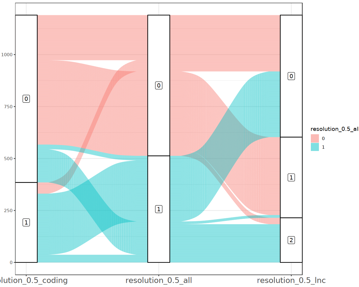
Display Differences Between Clustering Methods via Sankey Plot
options(repr.plot.width = 10, repr.plot.height = 8)

plot_data <- data.frame(resolution_0.5_coding=obj$resolution_0.5_coding,
                        resolution_0.5_all=obj$resolution_0.5_all,
                        resolution_0.5_lnc=obj$resolution_0.5_lnc)

p <- ggplot(plot_data,aes(axis1 = resolution_0.5_coding, axis2 =resolution_0.5_all, axis3 = resolution_0.5_lnc)) +
  geom_alluvium(aes(fill = resolution_0.5_all))+
  geom_stratum(width = 1/6) +
  geom_label(stat = "stratum", aes(label = after_stat(stratum)))+
  scale_x_discrete(limits = c("resolution_0.5_coding","resolution_0.5_all","resolution_0.5_lnc"),expand = c(0, 0))+
theme_bw()+
theme(axis.text.x = element_text(size=15))
p“Some strata appear at multiple axes.”
Warning message in to_lodes_form(data = data, axes = axis_ind, discern = params$discern):
“Some strata appear at multiple axes.”
Warning message in to_lodes_form(data = data, axes = axis_ind, discern = params$discern):
“Some strata appear at multiple axes.”
Compare Different Dimensionality Reduction Clustering via UMAP/tSNE Plots Results
UMAP Plot
options(repr.plot.width = 20, repr.plot.height = 6)
p=DimPlot(obj, group.by = "resolution_0.5_lnc", label = T, reduction = "UMAP_lnc",ncol=3)+
DimPlot(obj, group.by = "resolution_0.5_coding", label = T, reduction = "UMAP_coding")+
DimPlot(obj, group.by = "resolution_0.5_all", label = T, reduction = "UMAP_all")
p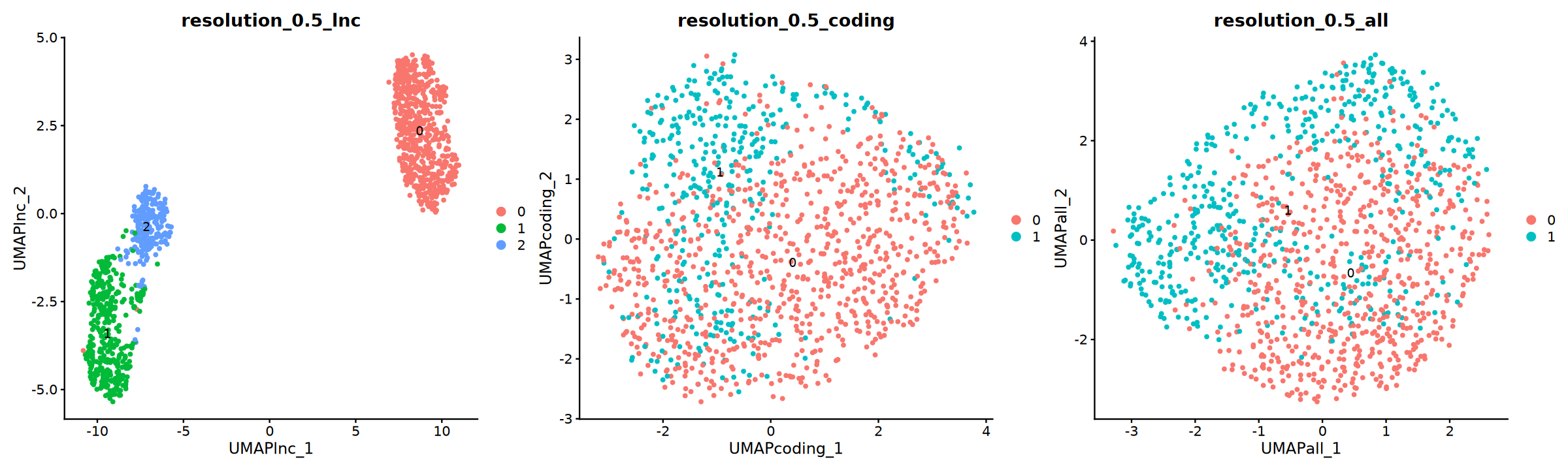
tSNE Plot
options(repr.plot.width = 20, repr.plot.height = 6)
p=DimPlot(obj, group.by = "resolution_0.5_lnc", label = T, reduction = "TSNE_lnc",ncol=3)+
DimPlot(obj, group.by = "resolution_0.5_coding", label = T, reduction = "TSNE_coding")+
DimPlot(obj, group.by = "resolution_0.5_all", label = T, reduction = "TSNE_all")
p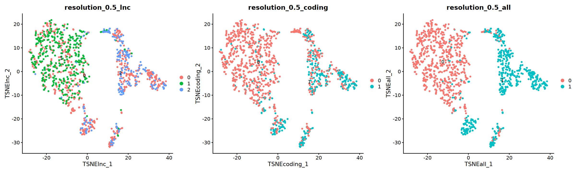
Save Clustering Results
New clustering results can be uploaded to the cloud platform and added as new meta information. Afterwards, understand gene expression and functional characteristics of different clusters through differential enrichment analysis, and obtain deeper feature information through other advanced analyses.
new_meta=obj@meta.data %>%
    as.data.frame() %>%
    select(barcode, resolution_0.5_lnc,resolution_0.5_coding,resolution_0.5_all)
head(new_meta)
write.csv(new_meta,file="clustering.csv",row.names=F,quote=F)| barcode | resolution_0.5_lnc | resolution_0.5_coding | resolution_0.5_all | |
|---|---|---|---|---|
| <chr> | <fct> | <fct> | <fct> | |
| AAACGAAGTTTCGCTC-1_1 | AAACGAAGTTTCGCTC-1_1 | 0 | 1 | 1 |
| AAAGAACAGAGCAGCT-1_1 | AAAGAACAGAGCAGCT-1_1 | 0 | 1 | 1 |
| AAAGGATGTTAATCGC-1_1 | AAAGGATGTTAATCGC-1_1 | 0 | 1 | 1 |
| AAAGGGCAGCCTTGAT-1_1 | AAAGGGCAGCCTTGAT-1_1 | 0 | 1 | 1 |
| AAAGGTACAGCACACC-1_1 | AAAGGTACAGCACACC-1_1 | 0 | 1 | 1 |
| AAATGGACACAGTGAG-1_1 | AAATGGACACAGTGAG-1_1 | 0 | 1 | 1 |
sessionInfo()Platform: x86_64-conda-linux-gnu (64-bit)
Running under: Debian GNU/Linux 12 (bookworm)
Matrix products: default
BLAS/LAPACK: /PROJ2/FLOAT/guopingfan/micromamba/env_files/envs/R_4.4.1/lib/libopenblasp-r0.3.30.so; LAPACK version 3.12.0
locale:
[1] LC_CTYPE=C.UTF-8 LC_NUMERIC=C LC_TIME=C.UTF-8
[4] LC_COLLATE=C.UTF-8 LC_MONETARY=C.UTF-8 LC_MESSAGES=C.UTF-8
[7] LC_PAPER=C.UTF-8 LC_NAME=C LC_ADDRESS=C
[10] LC_TELEPHONE=C LC_MEASUREMENT=C.UTF-8 LC_IDENTIFICATION=C
time zone: Asia/Shanghai
tzcode source: system (glibc)
attached base packages:
[1] stats graphics grDevices utils datasets methods base
other attached packages:
[1] future_1.67.0 ggalluvial_0.12.5 RColorBrewer_1.1-3 lubridate_1.9.4
[5] forcats_1.0.0 stringr_1.6.0 purrr_1.1.0 readr_2.1.5
[9] tidyr_1.3.1 tibble_3.3.0 tidyverse_2.0.0 dplyr_1.1.4
[13] plotly_4.11.0 ggplot2_3.5.2 harmony_1.2.1 Rcpp_1.1.0
[17] Seurat_5.3.0 SeuratObject_5.1.0 sp_2.2-0 repr_1.1.7
loaded via a namespace (and not attached):
[1] jsonlite_2.0.0 magrittr_2.0.3 spatstat.utils_3.1-5
[4] farver_2.1.2 ragg_1.3.3 vctrs_0.6.5
[7] ROCR_1.0-11 Cairo_1.6-2 spatstat.explore_3.5-2
[10] base64enc_0.1-3 htmltools_0.5.8.1 sctransform_0.4.2
[13] parallelly_1.45.1 KernSmooth_2.23-26 htmlwidgets_1.6.4
[16] ica_1.0-3 plyr_1.8.9 zoo_1.8-14
[19] uuid_1.2-1 igraph_2.0.3 mime_0.13
[22] lifecycle_1.0.4 pkgconfig_2.0.3 Matrix_1.6-5
[25] R6_2.6.1 fastmap_1.2.0 fitdistrplus_1.2-4
[28] shiny_1.11.1 digest_0.6.37 colorspace_2.1-1
[31] patchwork_1.3.2 tensor_1.5.1 RSpectra_0.16-2
[34] irlba_2.3.5.1 textshaping_0.4.0 labeling_0.4.3
[37] progressr_0.18.0 spatstat.sparse_3.1-0 timechange_0.3.0
[40] httr_1.4.7 polyclip_1.10-7 abind_1.4-8
[43] compiler_4.3.3 withr_3.0.2 fastDummies_1.7.5
[46] MASS_7.3-60.0.1 tools_4.3.3 lmtest_0.9-40
[49] otel_0.2.0 httpuv_1.6.15 future.apply_1.20.0
[52] goftest_1.2-3 glue_1.8.0 nlme_3.1-168
[55] promises_1.5.0 grid_4.3.3 pbdZMQ_0.3-13
[58] Rtsne_0.17 cluster_2.1.8.1 reshape2_1.4.4
[61] generics_0.1.4 gtable_0.3.6 spatstat.data_3.1-9
[64] tzdb_0.5.0 data.table_1.17.8 hms_1.1.3
[67] spatstat.geom_3.5-0 RcppAnnoy_0.0.22 ggrepel_0.9.6
[70] RANN_2.6.2 pillar_1.11.1 spam_2.11-1
[73] IRdisplay_1.1 RcppHNSW_0.6.0 later_1.4.2
[76] splines_4.3.3 lattice_0.22-7 survival_3.8-3
[79] deldir_2.0-4 tidyselect_1.2.1 miniUI_0.1.2
[82] pbapply_1.7-4 gridExtra_2.3 scattermore_1.2
[85] matrixStats_1.5.0 stringi_1.8.7 lazyeval_0.2.2
[88] evaluate_1.0.5 codetools_0.2-20 cli_3.6.5
[91] uwot_0.2.3 IRkernel_1.3.2 xtable_1.8-4
[94] reticulate_1.43.0 systemfonts_1.3.1 dichromat_2.0-0.1
[97] globals_0.18.0 spatstat.random_3.4-1 png_0.1-8
[100] spatstat.univar_3.1-4 parallel_4.3.3 dotCall64_1.2
[103] listenv_0.10.0 viridisLite_0.4.2 scales_1.4.0
[106] ggridges_0.5.7 crayon_1.5.3 rlang_1.1.6
[109] cowplot_1.2.0
References
[1] https://mp.weixin.qq.com/s/-a9kNKdsnKp6RH_rVpVsdA
[2] Bitar M, Rivera IS, Almeida I, Shi W, Ferguson K, Beesley J, Lakhani SR, Edwards SL, French JD. Redefining normal breast cell populations using long noncoding RNAs. Nucleic Acids Res. 2023 Jul 7;51(12):6389-6410. doi: 10.1093/nar/gkad339. PMID: 37144467; PMCID: PMC10325898.
[3] Aghagolzadeh P, Plaisance I, Bernasconi R, Treibel TA, Pulido Quetglas C, Wyss T, Wigger L, Nemir M, Sarre A, Chouvardas P, Johnson R, González A, Pedrazzini T. Assessment of the Cardiac Noncoding Transcriptome by Single-Cell RNA Sequencing Identifies FIXER, a Conserved Profibrogenic Long Noncoding RNA. Circulation. 2023 Aug 29;148(9):778-797. doi: 10.1161/CIRCULATIONAHA.122.062601. Epub 2023 Jul 10. PMID: 37427428.