单细胞精细解析：基于 LncRNA 表达特征的细胞分群策略

作者: SeekGene

时长: 16 分钟

字数: 3.2k 字

更新: 2026-02-28

阅读: 0 次

全序列转录组 Notebooks 基础分析

本文探讨在单细胞 RNA 测序分析中，除传统高变基因外，利用长链非编码 RNA 进行细胞分群的补充策略。LncRNA 表达具有更高的细胞状态特异性，有助于识别传统方法难以分辨的精细亚群；同时，其表达能直接关联细胞的表观遗传调控活性，为分群提供功能解释。当传统分群分辨率不足时，此方法有助于发现新型细胞状态或生物标志物。

例如，有研究 [1] 就用这个方法找到了新的细胞亚群和关键的 LncRNA 标志物；另一项研究 [2] 也通过 LncRNA 区分出了不同特性的细胞亚群。

这里推荐两步分群法：先以经典高变基因确定主要细胞类型，再在目标亚群内使用 LncRNA 进行二次分群。该策略可排除主要类型间的背景干扰，聚焦于同一谱系内部的异质性，从而更精准地解析细胞功能状态、发育轨迹或病理转变。

这里使用寻因公共数据来作为示例，LncRNA 分群适用于 DD3 转录组 / DD 全序列转录组 / DD5 转录组等多种数据类型，很多 LncRNA 基因都是有 poly-A 尾的，常规单细胞 RNA 捕获手段得到的数据可以满足分群分析。

options(repr.plot.width = 6, repr.plot.height = 6)

代码示例

加载所需 R 包

library(Seurat)
library(harmony)
library(plotly)
library(ggplot2)
library(dplyr)
library(tidyverse)
library(RColorBrewer)
library(ggalluvial)

读取 RDS 数据

obj=readRDS("../../../data/流程编号/input.rds")
meta=read.delim("../../../data/流程编号/meta.tsv")

rownames(meta)=meta$barcode
obj=AddMetaData(obj,metadata = meta)

对所有基因计算高变特征 (Variable Features)

obj <- FindVariableFeatures(obj, nfeatures = dim(obj)[1], verbose = FALSE)
hvg_all_features <- VariableFeatures(obj)
head(hvg_all_features)

output

Warning message:
“The \`slot\` argument of \`GetAssayData()\` is deprecated as of SeuratObject 5.0.0.
ℹ Please use the \`layer\` argument instead.
ℹ The deprecated feature was likely used in the Seurat package.
Please report the issue at .”

'IGHV4-59'
'IGKV1D-39'
'IGHV4-61'
'IGHV3-30'
'PTGDS'
'IGKV4-1'

读取基因类型

gene_biotype = read.csv("../GRCh38_gene_biotype.csv")
##人类GRCh38基因组可以直接读取下列数据
#gene_biotype = read.csv("https://seekgene-public.oss-cn-beijing.aliyuncs.com/software/FAST/GRCh38_gene_biotype.csv")
##小鼠mm10基因组可以直接读取下列数据
#gene_biotype = read.csv("https://seekgene-public.oss-cn-beijing.aliyuncs.com/software/FAST/mm10_gene_biotype.csv")
head(gene_biotype)
dim(gene_biotype)

A data.frame: 6 × 3
	gene_id	gene_type	gene_name
	<chr>	<chr>	<chr>
1	ENSG00000243485	lncRNA	MIR1302-2HG
2	ENSG00000237613	lncRNA	FAM138A
3	ENSG00000186092	protein_coding	OR4F5
4	ENSG00000238009	lncRNA	AL627309.1
5	ENSG00000239945	lncRNA	AL627309.3
6	ENSG00000239906	lncRNA	AL627309.2

36601
3

##筛选仅在rds中存在的基因，并按照hvg_all_features排序
all_genes=rownames(obj)
gene_biotype <- gene_biotype %>% filter(gene_name %in% hvg_all_features)
gene_biotype <- gene_biotype[match(hvg_all_features, gene_biotype$gene_name, nomatch = 0), ]
head(gene_biotype)

A data.frame: 6 × 3
	gene_id	gene_type	gene_name
	<chr>	<chr>	<chr>
13345	ENSG00000224373	IG_V_gene	IGHV4-59
2547	ENSG00000251546	IG_V_gene	IGKV1D-39
13346	ENSG00000211970	IG_V_gene	IGHV4-61
13331	ENSG00000270550	IG_V_gene	IGHV3-30
9429	ENSG00000107317	protein_coding	PTGDS
2522	ENSG00000211598	IG_V_gene	IGKV4-1

分别选择 Top 2000 的 LncRNA 基因、Protein-coding 基因、所有基因

top_2000_coding_RNA <- gene_biotype %>%
    filter(gene_type == "protein_coding")  %>%
    select(gene_name) %>%
    top_n(2000) %>%
    pull()
top_2000_lnc_RNA <- gene_biotype %>%
    filter(gene_type == "lncRNA")  %>%
    select(gene_name) %>%
    top_n(2000) %>%
    pull()
top_2000_all <- gene_biotype %>%
    select(gene_name) %>%
    top_n(2000) %>%
    pull()

output

Selecting by gene_name
Selecting by gene_name
Selecting by gene_name

redu="harmony" #如果rds是没有去除批次的，这里指定pca
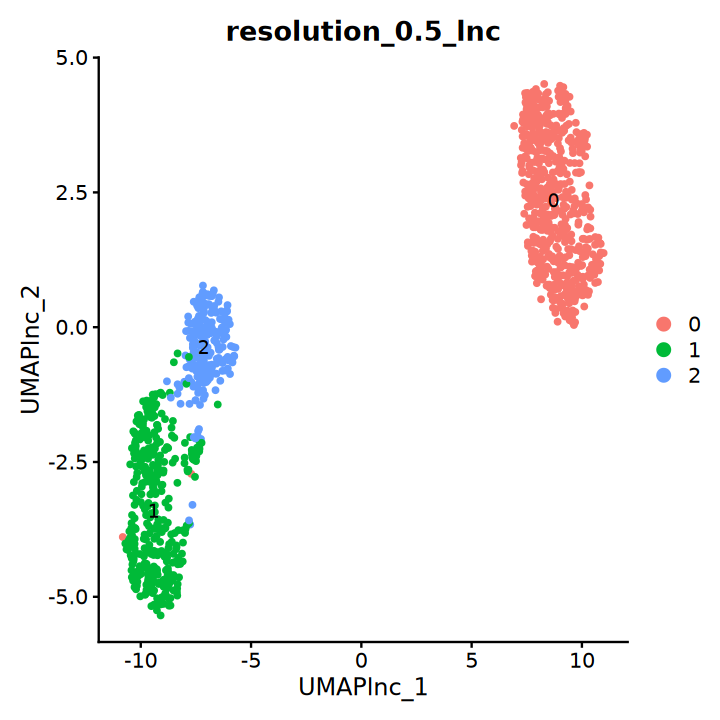
resolution_=0.5 #统一设置0.5的分辨率

基于 Top 2000 Lnc 基因做降维聚类

VariableFeatures(obj) <- top_2000_lnc_RNA

obj <- RunUMAP(object = obj,
               assay = "RNA",
               reduction = redu,
               features  = top_2000_lnc_RNA,
               verbose = FALSE)
obj <- RunTSNE(object = obj,
               assay = "RNA",
               reduction = redu,
               features  = top_2000_lnc_RNA,
               verbose = FALSE)
obj <- FindNeighbors(object = obj,
                     assay = "RNA",
                     reduction = redu,
                     dims = NULL,
                     features  = top_2000_lnc_RNA,
                     verbose = FALSE)
obj <- FindClusters(object = obj,
                    resolution = 0.5,
                    cluster.name = "resolution_0.5_lnc",
                    verbose = FALSE) 


embed <- Embeddings(obj, reduction = "umap")
obj[["UMAP_lnc"]] <- CreateDimReducObject(embeddings = embed, key = "UMAPlnc_", assay = DefaultAssay(obj))

embed <- Embeddings(obj, reduction = "tsne")
obj[["TSNE_lnc"]] <- CreateDimReducObject(embeddings = embed, key = "TSNElnc_", assay = DefaultAssay(obj))

DimPlot(obj, group.by = "resolution_0.5_lnc", label = T, reduction = "UMAP_lnc")

output

Warning message:
“The default method for RunUMAP has changed from calling Python UMAP via reticulate to the R-native UWOT using the cosine metric
To use Python UMAP via reticulate, set umap.method to 'umap-learn' and metric to 'correlation'
This message will be shown once per session”

基于 top 2000 coding 基因做降维聚类

VariableFeatures(obj) <- top_2000_coding_RNA

obj <- RunUMAP(object = obj,
               assay = "RNA",
               reduction = redu,
               features  = top_2000_coding_RNA,
               verbose = FALSE)
obj <- RunTSNE(object = obj,
               assay = "RNA",
               reduction = redu,
               features  = top_2000_coding_RNA,
               verbose = FALSE)
obj <- FindNeighbors(object = obj,
                     assay = "RNA",
                     reduction = redu,
                     dims = NULL,
                     features  = top_2000_coding_RNA,
                     verbose = FALSE)
obj <- FindClusters(object = obj,
                    resolution = 0.5,
                    cluster.name = "resolution_0.5_coding",
                    verbose = FALSE)


embed <- Embeddings(obj, reduction = "umap")
obj[["UMAP_coding"]] <- CreateDimReducObject(embeddings = embed, key = "UMAPcoding_", assay = DefaultAssay(obj))

embed <- Embeddings(obj, reduction = "tsne")
obj[["TSNE_coding"]] <- CreateDimReducObject(embeddings = embed, key = "TSNEcoding_", assay = DefaultAssay(obj))

DimPlot(obj, group.by = "resolution_0.5_coding", label = T, reduction = "UMAP_coding")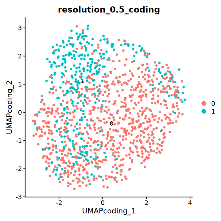

基于 top 2000 所有基因做降维聚类

VariableFeatures(obj) <- top_2000_all

obj <- RunUMAP(object = obj,
               assay = "RNA",
               reduction = redu,
               features  = top_2000_all,
               verbose = FALSE)
obj <- RunTSNE(object = obj,
               assay = "RNA",
               reduction = redu,
               features  = top_2000_all,
               verbose = FALSE)
obj <- FindNeighbors(object = obj,
                     assay = "RNA",
                     reduction = redu,
                     dims = NULL,
                     features  = top_2000_all,
                     verbose = FALSE)
obj <- FindClusters(object = obj,
                    resolution = 0.5,
                    cluster.name = "resolution_0.5_all",
                    verbose = FALSE) 

embed <- Embeddings(obj, reduction = "umap")
obj[["UMAP_all"]] <- CreateDimReducObject(embeddings = embed, key = "UMAPall_", assay = DefaultAssay(obj))

embed <- Embeddings(obj, reduction = "tsne")
obj[["TSNE_all"]] <- CreateDimReducObject(embeddings = embed, key = "TSNEall_", assay = DefaultAssay(obj))

DimPlot(obj, group.by = "resolution_0.5_all", label = T, reduction = "UMAP_all")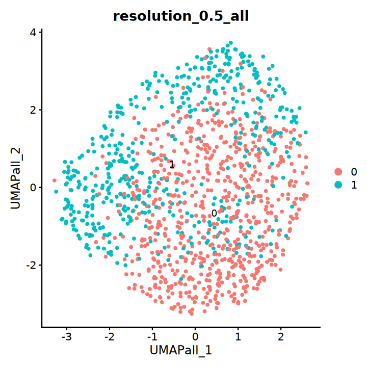

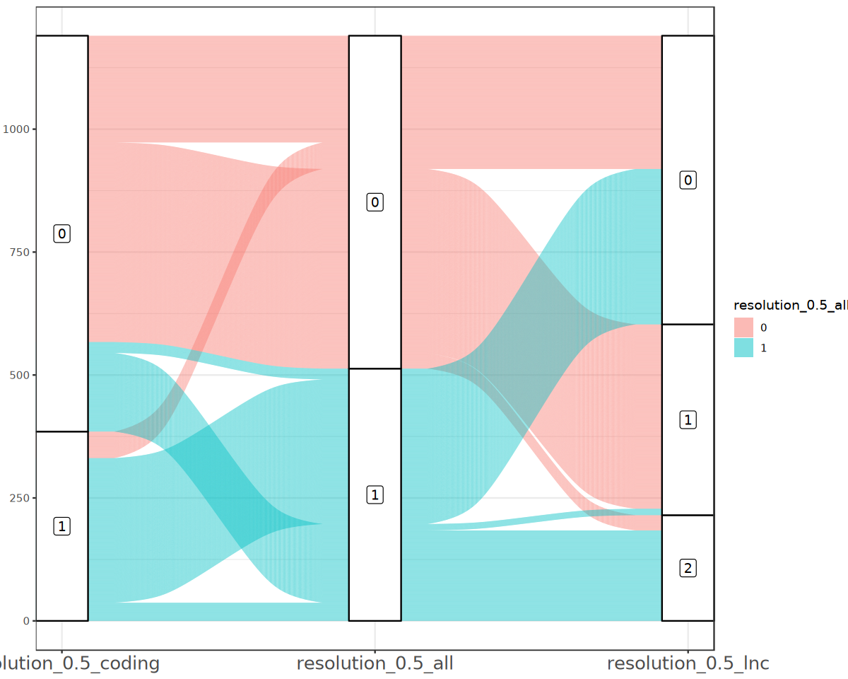
通过桑基图展示不同分群方式的区别

options(repr.plot.width = 10, repr.plot.height = 8)

plot_data <- data.frame(resolution_0.5_coding=obj$resolution_0.5_coding,
                        resolution_0.5_all=obj$resolution_0.5_all,
                        resolution_0.5_lnc=obj$resolution_0.5_lnc)

p <- ggplot(plot_data,aes(axis1 = resolution_0.5_coding, axis2 =resolution_0.5_all, axis3 = resolution_0.5_lnc)) +
  geom_alluvium(aes(fill = resolution_0.5_all))+
  geom_stratum(width = 1/6) +
  geom_label(stat = "stratum", aes(label = after_stat(stratum)))+
  scale_x_discrete(limits = c("resolution_0.5_coding","resolution_0.5_all","resolution_0.5_lnc"),expand = c(0, 0))+
theme_bw()+
theme(axis.text.x = element_text(size=15))
p

output

Warning message in to_lodes_form(data = data, axes = axis_ind, discern = params$discern):
“Some strata appear at multiple axes.”
Warning message in to_lodes_form(data = data, axes = axis_ind, discern = params$discern):
“Some strata appear at multiple axes.”
Warning message in to_lodes_form(data = data, axes = axis_ind, discern = params$discern):
“Some strata appear at multiple axes.”

通过 umap/tsne 图对比不同降维分群结果

umap 图

options(repr.plot.width = 20, repr.plot.height = 6)
p=DimPlot(obj, group.by = "resolution_0.5_lnc", label = T, reduction = "UMAP_lnc",ncol=3)+
DimPlot(obj, group.by = "resolution_0.5_coding", label = T, reduction = "UMAP_coding")+
DimPlot(obj, group.by = "resolution_0.5_all", label = T, reduction = "UMAP_all")
p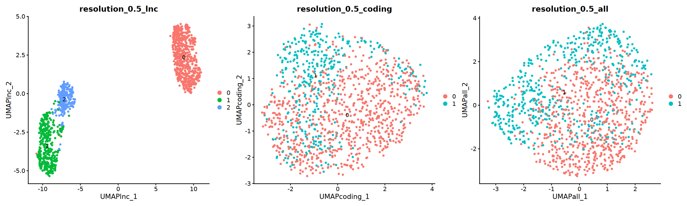

tsne 图

options(repr.plot.width = 20, repr.plot.height = 6)
p=DimPlot(obj, group.by = "resolution_0.5_lnc", label = T, reduction = "TSNE_lnc",ncol=3)+
DimPlot(obj, group.by = "resolution_0.5_coding", label = T, reduction = "TSNE_coding")+
DimPlot(obj, group.by = "resolution_0.5_all", label = T, reduction = "TSNE_all")
p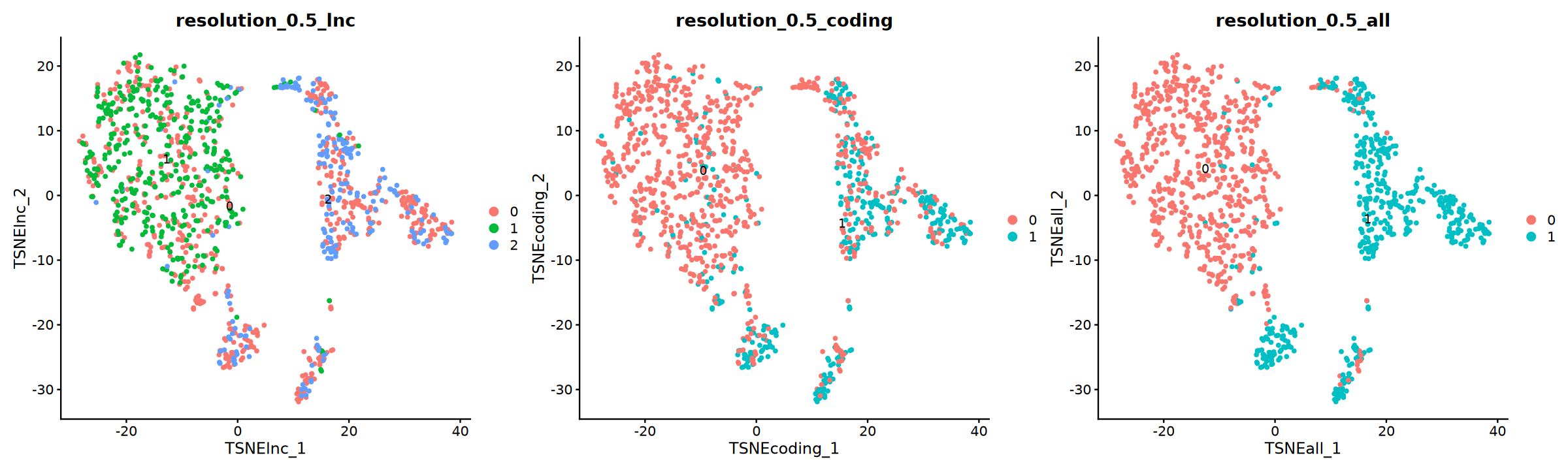

保存分群结果

新的分群结果可以上传到云平台，添加作为新的 meta 信息。之后通过差异富集分析了解不同 cluster 的基因表达、功能特征，通过其他高级分析获取更深层次的特征信息。

new_meta=obj@meta.data %>%
    as.data.frame() %>%
    select(barcode, resolution_0.5_lnc,resolution_0.5_coding,resolution_0.5_all)
head(new_meta)
write.csv(new_meta,file="clustering.csv",row.names=F,quote=F)

A data.frame: 6 × 4
	barcode	resolution_0.5_lnc	resolution_0.5_coding	resolution_0.5_all
	<chr>	<fct>	<fct>	<fct>
AAACGAAGTTTCGCTC-1_1	AAACGAAGTTTCGCTC-1_1	0	1	1
AAAGAACAGAGCAGCT-1_1	AAAGAACAGAGCAGCT-1_1	0	1	1
AAAGGATGTTAATCGC-1_1	AAAGGATGTTAATCGC-1_1	0	1	1
AAAGGGCAGCCTTGAT-1_1	AAAGGGCAGCCTTGAT-1_1	0	1	1
AAAGGTACAGCACACC-1_1	AAAGGTACAGCACACC-1_1	0	1	1
AAATGGACACAGTGAG-1_1	AAATGGACACAGTGAG-1_1	0	1	1

sessionInfo()

output

R version 4.3.3 (2024-02-29)
Platform: x86_64-conda-linux-gnu (64-bit)
Running under: Debian GNU/Linux 12 (bookworm)

Matrix products: default
BLAS/LAPACK: /PROJ2/FLOAT/guopingfan/micromamba/env_files/envs/R_4.4.1/lib/libopenblasp-r0.3.30.so; LAPACK version 3.12.0

locale:
[1] LC_CTYPE=C.UTF-8 LC_NUMERIC=C LC_TIME=C.UTF-8
[4] LC_COLLATE=C.UTF-8 LC_MONETARY=C.UTF-8 LC_MESSAGES=C.UTF-8
[7] LC_PAPER=C.UTF-8 LC_NAME=C LC_ADDRESS=C
[10] LC_TELEPHONE=C LC_MEASUREMENT=C.UTF-8 LC_IDENTIFICATION=C

time zone: Asia/Shanghai
tzcode source: system (glibc)

attached base packages:
[1] stats graphics grDevices utils datasets methods base

other attached packages:
[1] future_1.67.0 ggalluvial_0.12.5 RColorBrewer_1.1-3 lubridate_1.9.4
[5] forcats_1.0.0 stringr_1.6.0 purrr_1.1.0 readr_2.1.5
[9] tidyr_1.3.1 tibble_3.3.0 tidyverse_2.0.0 dplyr_1.1.4
[13] plotly_4.11.0 ggplot2_3.5.2 harmony_1.2.1 Rcpp_1.1.0
[17] Seurat_5.3.0 SeuratObject_5.1.0 sp_2.2-0 repr_1.1.7

loaded via a namespace (and not attached):
[1] jsonlite_2.0.0 magrittr_2.0.3 spatstat.utils_3.1-5
[4] farver_2.1.2 ragg_1.3.3 vctrs_0.6.5
[7] ROCR_1.0-11 Cairo_1.6-2 spatstat.explore_3.5-2
[10] base64enc_0.1-3 htmltools_0.5.8.1 sctransform_0.4.2
[13] parallelly_1.45.1 KernSmooth_2.23-26 htmlwidgets_1.6.4
[16] ica_1.0-3 plyr_1.8.9 zoo_1.8-14
[19] uuid_1.2-1 igraph_2.0.3 mime_0.13
[22] lifecycle_1.0.4 pkgconfig_2.0.3 Matrix_1.6-5
[25] R6_2.6.1 fastmap_1.2.0 fitdistrplus_1.2-4
[28] shiny_1.11.1 digest_0.6.37 colorspace_2.1-1
[31] patchwork_1.3.2 tensor_1.5.1 RSpectra_0.16-2
[34] irlba_2.3.5.1 textshaping_0.4.0 labeling_0.4.3
[37] progressr_0.18.0 spatstat.sparse_3.1-0 timechange_0.3.0
[40] httr_1.4.7 polyclip_1.10-7 abind_1.4-8
[43] compiler_4.3.3 withr_3.0.2 fastDummies_1.7.5
[46] MASS_7.3-60.0.1 tools_4.3.3 lmtest_0.9-40
[49] otel_0.2.0 httpuv_1.6.15 future.apply_1.20.0
[52] goftest_1.2-3 glue_1.8.0 nlme_3.1-168
[55] promises_1.5.0 grid_4.3.3 pbdZMQ_0.3-13
[58] Rtsne_0.17 cluster_2.1.8.1 reshape2_1.4.4
[61] generics_0.1.4 gtable_0.3.6 spatstat.data_3.1-9
[64] tzdb_0.5.0 data.table_1.17.8 hms_1.1.3
[67] spatstat.geom_3.5-0 RcppAnnoy_0.0.22 ggrepel_0.9.6
[70] RANN_2.6.2 pillar_1.11.1 spam_2.11-1
[73] IRdisplay_1.1 RcppHNSW_0.6.0 later_1.4.2
[76] splines_4.3.3 lattice_0.22-7 survival_3.8-3
[79] deldir_2.0-4 tidyselect_1.2.1 miniUI_0.1.2
[82] pbapply_1.7-4 gridExtra_2.3 scattermore_1.2
[85] matrixStats_1.5.0 stringi_1.8.7 lazyeval_0.2.2
[88] evaluate_1.0.5 codetools_0.2-20 cli_3.6.5
[91] uwot_0.2.3 IRkernel_1.3.2 xtable_1.8-4
[94] reticulate_1.43.0 systemfonts_1.3.1 dichromat_2.0-0.1
[97] globals_0.18.0 spatstat.random_3.4-1 png_0.1-8
[100] spatstat.univar_3.1-4 parallel_4.3.3 dotCall64_1.2
[103] listenv_0.10.0 viridisLite_0.4.2 scales_1.4.0
[106] ggridges_0.5.7 crayon_1.5.3 rlang_1.1.6
[109] cowplot_1.2.0

参考资料

[1] https://mp.weixin.qq.com/s/-a9kNKdsnKp6RH_rVpVsdA

[2] Bitar M, Rivera IS, Almeida I, Shi W, Ferguson K, Beesley J, Lakhani SR, Edwards SL, French JD. Redefining normal breast cell populations using long noncoding RNAs. Nucleic Acids Res. 2023 Jul 7;51(12):6389-6410. doi: 10.1093/nar/gkad339. PMID: 37144467; PMCID: PMC10325898.

[3] Aghagolzadeh P, Plaisance I, Bernasconi R, Treibel TA, Pulido Quetglas C, Wyss T, Wigger L, Nemir M, Sarre A, Chouvardas P, Johnson R, González A, Pedrazzini T. Assessment of the Cardiac Noncoding Transcriptome by Single-Cell RNA Sequencing Identifies FIXER, a Conserved Profibrogenic Long Noncoding RNA. Circulation. 2023 Aug 29;148(9):778-797. doi: 10.1161/CIRCULATIONAHA.122.062601. Epub 2023 Jul 10. PMID: 37427428.

单细胞精细解析：基于 LncRNA 表达特征的细胞分群策略 ​

代码示例 ​

加载所需 R 包 ​

读取 RDS 数据 ​

对所有基因计算高变特征 (Variable Features) ​

读取基因类型 ​

分别选择 Top 2000 的 LncRNA 基因、Protein-coding 基因、所有基因 ​

基于 Top 2000 Lnc 基因做降维聚类 ​

基于 top 2000 coding 基因做降维聚类 ​

基于 top 2000 所有基因做降维聚类 ​

通过桑基图展示不同分群方式的区别 ​

通过 umap/tsne 图对比不同降维分群结果 ​

umap 图 ​

tsne 图 ​

保存分群结果 ​

参考资料 ​

单细胞精细解析：基于 LncRNA 表达特征的细胞分群策略

代码示例

加载所需 R 包

读取 RDS 数据

对所有基因计算高变特征 (Variable Features)

读取基因类型

分别选择 Top 2000 的 LncRNA 基因、Protein-coding 基因、所有基因

基于 Top 2000 Lnc 基因做降维聚类

基于 top 2000 coding 基因做降维聚类

基于 top 2000 所有基因做降维聚类

通过桑基图展示不同分群方式的区别

通过 umap/tsne 图对比不同降维分群结果

umap 图

tsne 图

保存分群结果

参考资料