scRNA-seq Multi-sample Integration Tutorial (Seurat / Harmony)

Author: SeekGene

Time: 15 min

Words: 3.0k words

Updated: 2026-02-27

Reads: 0 times

3' scRNA-seq 5' + Immune Profiling Analysis Guide Data Integration FFPE scRNA-seq Notebooks Spatial-seq scATAC + RNA-seq scFAST-seq scMethyl + RNA-seq

Environment Setup

Load R Packages

Please select the 'common_r' environment for this tutorial.

# Load required R packages
suppressPackageStartupMessages({
  library(Seurat)
  library(dplyr)
  library(ggplot2)
  library(patchwork)
  library(harmony)
})

# Set random seed
set.seed(1234)

# Set Seurat options (Note: 8000 * 1024^2 is approx 8GB)
options(future.globals.maxSize = 8000 * 1024^2)  # 8GB

my36colors <-c( '#E5D2DD', '#53A85F', '#F1BB72', '#F3B1A0', '#D6E7A3', '#57C3F3', '#476D87',
                '#E95C59', '#E59CC4', '#AB3282', '#23452F', '#BD956A', '#8C549C', '#585658',
                '#9FA3A8', '#E0D4CA', '#5F3D69', '#C5DEBA', '#58A4C3', '#E4C755', '#F7F398',
                '#AA9A59', '#E63863', '#E39A35', '#C1E6F3', '#6778AE', '#91D0BE', '#B53E2B',
                '#712820', '#DCC1DD', '#CCE0F5', '#CCC9E6', '#625D9E', '#68A180', '#3A6963',
                '#968175', "#6495ED", "#FFC1C1",'#f1ac9d','#f06966','#dee2d1','#6abe83','#39BAE8','#B9EDF8','#221a12',
                '#b8d00a','#74828F','#96C0CE','#E95D22','#017890')

Data Loading

This tutorial provides two data input methods to meet different user needs. Choose the one that suits you:

Cloud Platform RDS File Loading

Data Characteristics:

• RDS files are standard Seurat object files
• Data has been preprocessed and multiple samples merged
• Can be used directly for downstream analysis, or expression matrix can be extracted for re-integration

Applicable Scenarios:

• When you cannot obtain standard filtered_feature_bc_matrix files
• When you want to integrate existing cloud platform data for learning
• When you need to quickly re-run scRNA-seq integration analysis

Notes:

• For data mounting and RDS file reading, please refer to the Jupyter usage tutorial

For example, project data at /home/demo-SeekGene-com/workspace/data/AY1752565399550/

input <- readRDS("/home/demo-seekgene-com/workspace/data/AY1752565399550/input.rds")
meta <- read.table("/home/demo-seekgene-com/workspace/data/AY1752565399550/meta.tsv", header=TRUE, sep="\t", row.names = 1)
data <- AddMetaData(input,meta)
data <- CreateSeuratObject(counts = input@assay$RNA@counts, meta.data=meta)
seurat_list <- SplitObject(data, split.by = "Sample")
# Remove unnecessary data to free up memory
rm(data,input)
gc()

Standard filtered_feature_bc_matrix File Loading

Applicable Scenarios:

• When you have standard gene expression matrix files
• When you want to independently complete scRNA-seq multi-sample integration and batch correction
• When you need a complete workflow from raw data to integration analysis

Note:

• Ensure the file structure for samples is as follows:

scRNA-seq Data (Gene Expression Matrix)
├── S127/
│ ├── filtered_feature_bc_matrix/
│ │ ├── barcodes.tsv.gz (Cell Barcodes)
│ │ ├── features.tsv.gz (Feature List)
│ │ └── matrix.mtx.gz (Sparse Count Matrix)
├── S44R/
│ ├── filtered_feature_bc_matrix/
│ │ ├── barcodes.tsv.gz
│ │ ├── features.tsv.gz
│ │ └── matrix.mtx.gz

# Define sample names
sample_names <- c('S127', 'S44R')
# Create an empty list to store Seurat objects for each sample
seurat_list <- list()

for (sample in sample_names) {
  # Construct file paths
  data_path <- file.path(sample, 'filtered_feature_bc_matrix')

  # Read expression matrix files
  counts <- Read10X(data.dir = data_path)
  
  # Create Seurat object
  rna_obj <- CreateSeuratObject(
    counts = counts,
    project = sample,
    min.cells = 3,      # Filter genes expressed in fewer than 3 cells
    min.features = 200   # Filter cells with fewer than 200 expressed genes
  )
  
  # Add sample ID
  rna_obj$Sample <- sample
  rna_obj$orig.ident <- sample
  # Add Seurat object to list
  seurat_list[[sample]] <- rna_obj
  # Clear rna_obj object
  rm(rna_obj)
  gc()
}

Quality Control

Before integration, each sample's data needs to be 'cleaned':

• QC (Quality Control): Remove low-quality cells (e.g., high mitochondrial content, background, or doublets)

Calculate QC Metrics

Calculate key QC metrics for each sample for subsequent cell filtering.

Common QC Metrics:

• nCount_ATAC: Total ATAC counts; extremely low or high values indicate anomalies.
• percent.mt: Mitochondrial gene percentage (usually <20%)
• nFeature_RNA: Total RNA features (usually between 200-10000)
• nCount_RNA: Total RNA counts (usually between 200-10000)

# Perform QC on each object in seurat_list
seurat_list <- lapply(seurat_list, function(x) {
  x[["percent.mt"]] <- PercentageFeatureSet(x, pattern = "^MT-")
  return(x)
})

QC Metrics Visualization

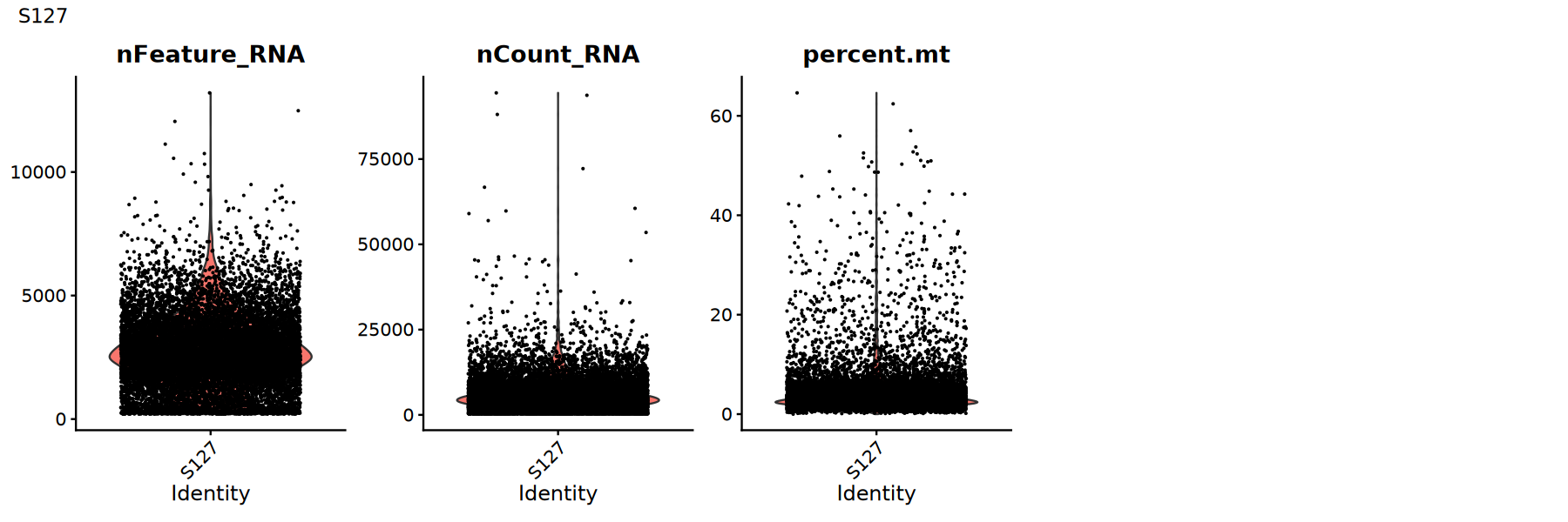
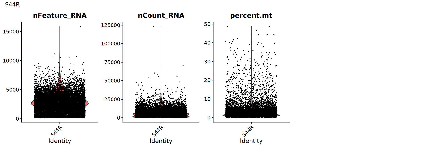
Use violin plots to view distribution/outliers of QC metrics to determine appropriate thresholds:

Suggestions:

• Look for obvious long tails or bimodal distributions
• Try multiple thresholds and compare if downstream clustering/UMAP is clearer

options(repr.plot.width = 15, repr.plot.height = 5)
for (sample_name in names(seurat_list)) {
  seurat_obj <- seurat_list[[sample_name]]

  # Violin plot showing QC metric distribution
  p1 <- VlnPlot(
    object = seurat_obj,
    features = c('nFeature_RNA', 'nCount_RNA', 'percent.mt'),
    pt.size = 0.1,
    ncol = 5
  )
  print(p1+plot_annotation(title = sample_name))
}

Filter Low-Quality Cells

Filter low-quality cells based on QC metrics. Thresholds should be adjusted based on data characteristics and violin plots above.

# Use lapply for QC filtering
seurat_list <- lapply(seurat_list, function(x) {
  # Record cell count before filtering
  cells_before <- ncol(x)
  
  # Quality Control Filtering
  x <- subset( x,subset = nFeature_RNA > 200 &     # Gene count > 200
             nFeature_RNA < 8000 &    # Gene count < 8000
             nCount_RNA > 500 &       # UMI count > 500
             nCount_RNA < 30000 &     # UMI count < 30000
             percent.mt < 20         # Mitochondrial gene ratio < 20%
  )
  
  # Record cell count after filtering
  cells_after <- ncol(x)
  
  # Output filtering info
  cat('Filtering complete: Before', cells_before, 'cells, After', cells_after, 'cells\n')
  
  return(x)
})

output

过滤完成: 过滤前 13719 个细胞，过滤后 12722 个细胞
过滤完成: 过滤前 11830 个细胞，过滤后 11122 个细胞

Multi-sample Merging

In scRNA-seq analysis, multi-sample merging is a key prerequisite for integration.

Purpose of Merging:

• Merge data from multiple samples into a single Seurat object
• Prepare for subsequent batch correction and integration analysis
• Facilitate comparison with batch-corrected results

Important Notes:

• This step only performs simple data merging, not batch correction
• The merged object contains raw data from all samples
• Proceed with preprocessing steps like normalization, feature selection, PCA, and UMAP on merged data

# Merge all samples
suppressWarnings({
  suppressMessages({
      obj_merge <- merge(seurat_list[[1]], seurat_list[-1], merge.data = FALSE)
      obj_merge <- NormalizeData(obj_merge)
      obj_merge <- FindVariableFeatures(obj_merge, nfeatures = 2000)
      obj_merge <- ScaleData(obj_merge)
      obj_merge <- RunPCA(obj_merge)
        })
})

Data Integration

Now we integrate scRNA-seq data from multiple samples and perform dimensionality reduction and clustering. Two common methods are:

Integration Method Selection

CCA (Canonical Correlation Analysis) Integration:

• Integration based on Canonical Correlation Analysis
• Integrates by finding common variation patterns between samples
• Suitable for cases with large differences between samples
• Classic integration method in Seurat

Harmony Integration:

• Fast integration based on iterative clustering
• Corrects batch effects directly in reduced dimensional space
• High computational efficiency, suitable for large-scale data
• Preserves more biological variation

Method Selection Advice

• Harmony: Same platform different samples; faster for many samples or large datasets.
• CCA: Slower; recommended for severe batch effects, e.g., cross-platform data.

Integration using Harmony

Note: Choose either Harmony or CCA for batch correction.

# Define Harmony integration function
integrate_harmony <- function(obj) {
  DefaultAssay(obj) <- "RNA"
  obj <- RunHarmony(obj, "Sample")  
  obj <- RunUMAP(obj, reduction = "harmony",
                  dims = 1:30)
  #obj <- RunTSNE(obj, reduction = "harmony",dims = 1:30,check_duplicates = FALSE)
  # RNA data clustering
  obj <- FindNeighbors(object = obj, reduction = 'harmony', dims = 1:30)
  obj <- FindClusters(object = obj, verbose = FALSE, algorithm = 3,resolution = 0.5)
  return(obj)
}

# Execute Harmony integration analysis
suppressWarnings({
  suppressMessages({
      obj_integrated = integrate_harmony(obj_merge)
      })
    })

Integration using CCA

Note: Choose either Harmony or CCA for batch correction.

# Switch to RNA assay
suppressWarnings({
  suppressMessages({
      objs <- lapply(seurat_list, function(x) {
          DefaultAssay(x) <- "RNA"
          return(x)
      })

      cat('Total cells after merge:', ncol(obj_merge), '\n')
      # Define CCA integration function
      integrate_cca <- function(objs) {
          objs <- lapply(objs, function(x) {
            x <- NormalizeData(x, verbose = FALSE)
            x <- FindVariableFeatures(x,nfeatures = 2000,selection.method = "vst")
            return(x)
          })
          features <- Seurat::SelectIntegrationFeatures(object.list = objs)
          anchors <- Seurat::FindIntegrationAnchors(
              object.list = objs,
              anchor.features = features
          ) 
          obj <- Seurat::IntegrateData(anchorset = anchors)
          DefaultAssay(obj) <- "integrated"
          obj <- Seurat::ScaleData(obj, verbose = FALSE) %>%
          RunPCA(verbose = FALSE)
          # Perform UMAP on integrated data
          obj <- RunUMAP(obj, reduction = "pca", dims = 1:30)
          # RNA data clustering
          obj <- FindNeighbors(object = obj, dims = 1:30)
          obj <- FindClusters(object = obj, verbose = FALSE, algorithm = 3,resolution = 0.5)
          #obj <- RunTSNE(obj, reduction = "pca", dims = 1:30, check_duplicates = FALSE)
          return(obj)
          }
          # Execute CCA integration
          obj_integrated <- integrate_cca(seurat_list)

  })
})

output

合并后细胞总数: 23844

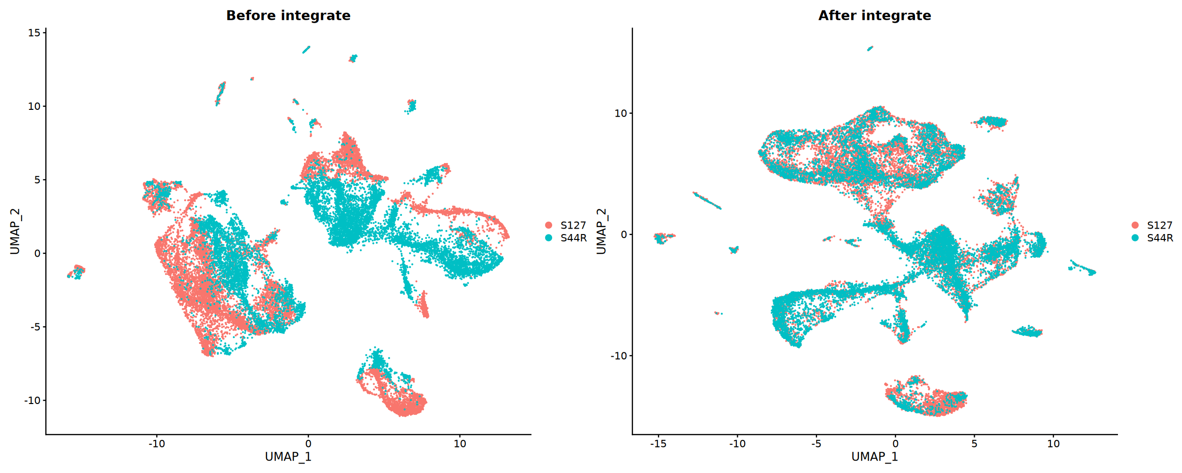
Integration Evaluation

Compare results before and after integration to evaluate effectiveness.

Evaluation Metrics:

• Sample Mixing: Distribution of cells from different samples in UMAP
• Batch Effect Removal: Clustering of technical replicates
• Biological Signal Retention: Separation of known cell types

cat('Starting visualization of integration results...', Sys.time(), '\n')
# Compare effects before and after integration
suppressWarnings({
  suppressMessages({
      obj_merge <- RunUMAP(obj_merge, reduction = "pca", dims = 1:30)
      })
    })
p1 <- DimPlot(obj_merge, group.by = "Sample") +
  ggtitle("Before integrate")

p2 <- DimPlot(obj_integrated, group.by = "Sample") +
  ggtitle("After integrate")

# Save comparison plots
pdf("integration_comparison.pdf", width = 16, height = 12)
print(p1 + p2)
dev.off()

options(repr.plot.width = 20, repr.plot.height = 8)
print(p1 + p2)

output

开始可视化整合结果... 1755238468

pdf: 2

Cell Type Annotation

Annotate cell types based on marker gene expression. Use differential expression on clusters to get candidate markers, then verify with literature/databases.

Define Marker Genes

Compile reference markers for common cell types (from literature, PanglaoDB, CellMarker, etc.) for visualization and interpretation.

eye_marker_integrated <- list(
  # ========== Photoreceptor Cells ==========
  "Rod_Photoreceptors" = c("RHO", "PDE6B", "CNGB1", "PDE6A", "NR2E3", "REEP6",
                          "RCVRN", "SAG", "NEB", "SLC24A3", "TRPM1"),
  "Cone_Photoreceptors" = c("ARR3", "GNAT2", "OPN1SW", "TRPM3"),

  # ========== Retinal Neurons ==========
  "Bipolar_Cells" = c("VSX1", "OTX2", "GRM6", "PRKCA",
                     "DLG2", "NRXN3", "RBFOX3", "FSTL4"),
  "Amacrine_Cells" = c("GAD1", "GAD2", "C1QL2", "TFAP2B", "SLC32A1"),
  "Horizontal_Cells" = c("ONECUT1", "LHX1", "CALB1", "NFIA"),
  "Retinal_Ganglion_Cells" = c("RBPMS", "THY1", "NEFL", "POU4F2"),

  # ========== Glial Cells ==========
  "Muller_Glia" = c("SLC1A3", "RLBP1", "SOX9", "CRYAB"),
  "Astrocytes" = c("GFAP", "AQP4", "S100B"),
  "Microglia" = c("TMEM119", "C1QA", "AIF1", "CX3CR1", "CD74",
                 "PTPRC", "CSF1R", "CCL3L1", "SPP1", "P2RY12"),

  # ========== Vascular and Support Cells ==========
  "Endothelial" = c("FLT1", "PODXL", "PLVAP", "KDR", "EGFL7",
                   "CLDN5", "PECAM1", "CDH5"),
  "Pericytes" = c("PDGFRB", "RGS5", "CSPG4", "STAB1"),

  # ========== Epithelial Cells ==========
  "RPE" = c("RPE65", "BEST1", "PMEL", "TYRP1", "DCT", "SLC38A11"),
  #"Corneal_Epithelial" = c("KRT12", "KRT3"),
  "Corneal_Endothelial" = c("SLC4A11", "COL8A2", "ATP1A1"),
  "Conjunctival_Epithelial" = c("KRT13", "KRT19", "MUC5AC"),
  "Retinal_Progenitors" = c("VSX2", "PAX6","SOX2", "HES1", "NOTCH1"),  # Retinal Progenitors

  # ========== Lens Cells ==========
  "Lens_Epithelial" = c("CRYAA", "BFSP1", "MIP"),
  "Lens_Fiber" = c("CRYGS", "LIM2", "FN1"),

  # ========== Other Cells ==========
  "Melanocytes" = c("TYR", "MLANA", "MITF"),
  #"Erythrocytes" = c("HBB", "HBA1", "HBA2"),
  "ECM" = c("COL1A1", "COL3A1", "COL12A1", "COL1A2", "COL6A3")#,
  #"Others" = c("TTN", "CLCN5", "DCC", "MIAT")
)

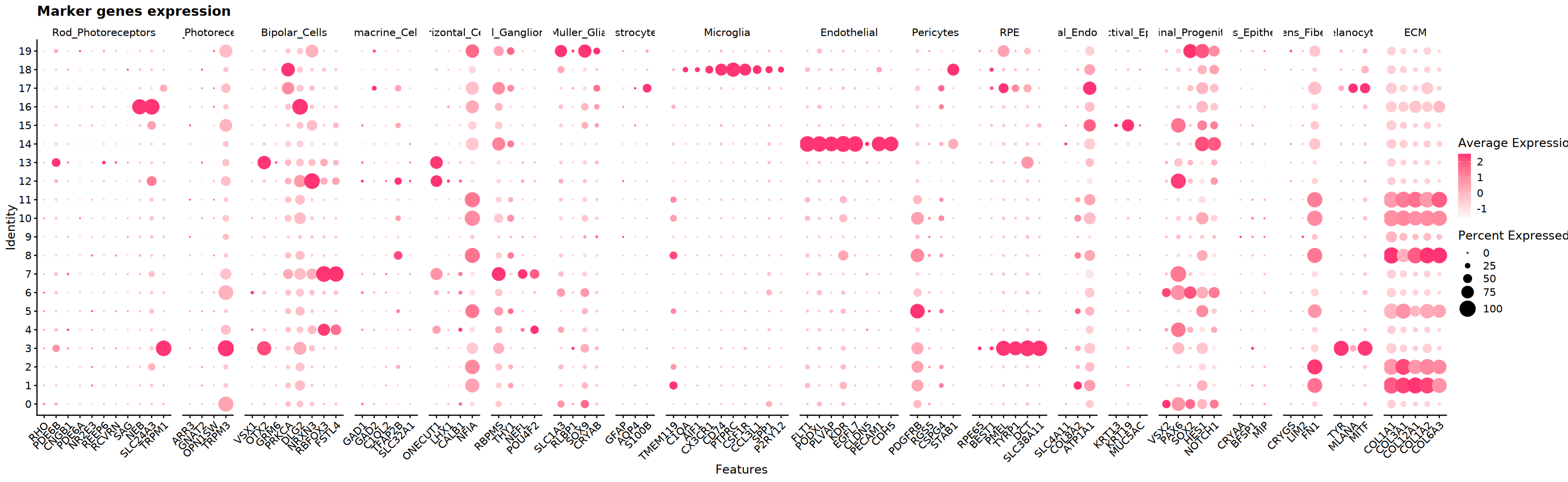
Marker Gene Expression Visualization

Display expression patterns of candidate markers in clusters (Violin/Dot/FeaturePlot) to assist in type assignment.

cat('Starting marker gene visualization...', Sys.time(), '\n')
# Create DotPlot to show marker gene expression
DefaultAssay(obj_integrated)="RNA"
p_dot <- DotPlot(
  obj_integrated,
  features = eye_marker_integrated,
  cols = c("#f8f8f8","#ff3472"),
  dot.scale = 8
) +
  RotatedAxis() +
  ggtitle("Marker genes expression") +
  theme(axis.text.x = element_text(angle = 45, hjust = 1))

# Save DotPlot
pdf("marker_genes_dotplot.pdf", width = 16, height = 8)
print(p_dot)
dev.off()
options(repr.plot.width = 26, repr.plot.height = 8)
print(p_dot)

cat('Marker gene visualization complete!', Sys.time(), '\n')

output

开始marker基因表达可视化... 1755238806

pdf: 2

marker基因表达可视化完成! 1755238807 

p3 <- DimPlot(obj_integrated,group.by = "seurat_clusters",label = T, cols = my36colors)+ggtitle("Clusters")
options(repr.plot.width = 10, repr.plot.height = 8)
print(p3)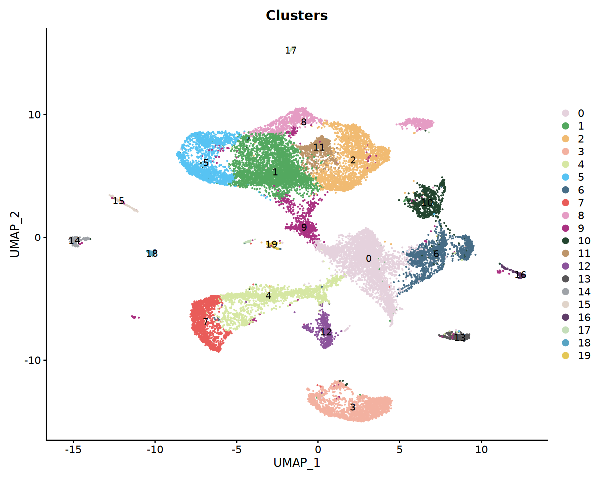

Cell Type Annotation

Annotate cell types combining cluster-level differential genes and reference markers; refine to subtypes or adjust resolution if needed.

cat('Starting cell type annotation...', Sys.time(), '\n')

# Annotate cell types based on clustering (adjust according to actual marker expression)
# Example provided here; adjust based on DotPlot results in practice
celltype_mapping <- c(
  "0" = "Retinal_Progenitors",
  "1" = "ECM",
  "2" = "ECM",
  "3" = "PRE",
  "4" = "Bipolar_Cells",
  "5" = "ECM",
  "6" = "Retinal_Progenitors",
  "7" = "Bipolar_Cells",
  "8" = "ECM",
  "9" = "Conjunctival_Epithelial",
  "10" = "ECM",
  "11" = "ECM",
  "12" = "Bipolar_Cells",
  "13" = "Doublets",
  "14" = "Endothelial",
  "15" = "Conjunctival_Epithelial",
  "16" = "Rod_Photoreceptors",
  "17" = "Astrocytes",
  "18" = "Microglia",
  "19" = "Muller_Glia"
)

# Apply cell type annotation
obj_integrated$celltype <- recode(
  obj_integrated$seurat_clusters,
  !!!celltype_mapping
)

output

开始细胞类型注释... 1755239393

Cell Type Annotation Visualization

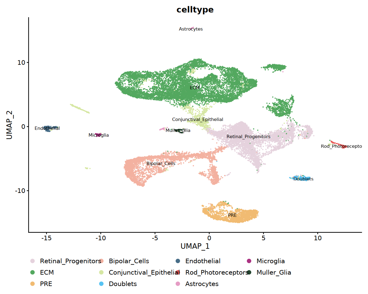
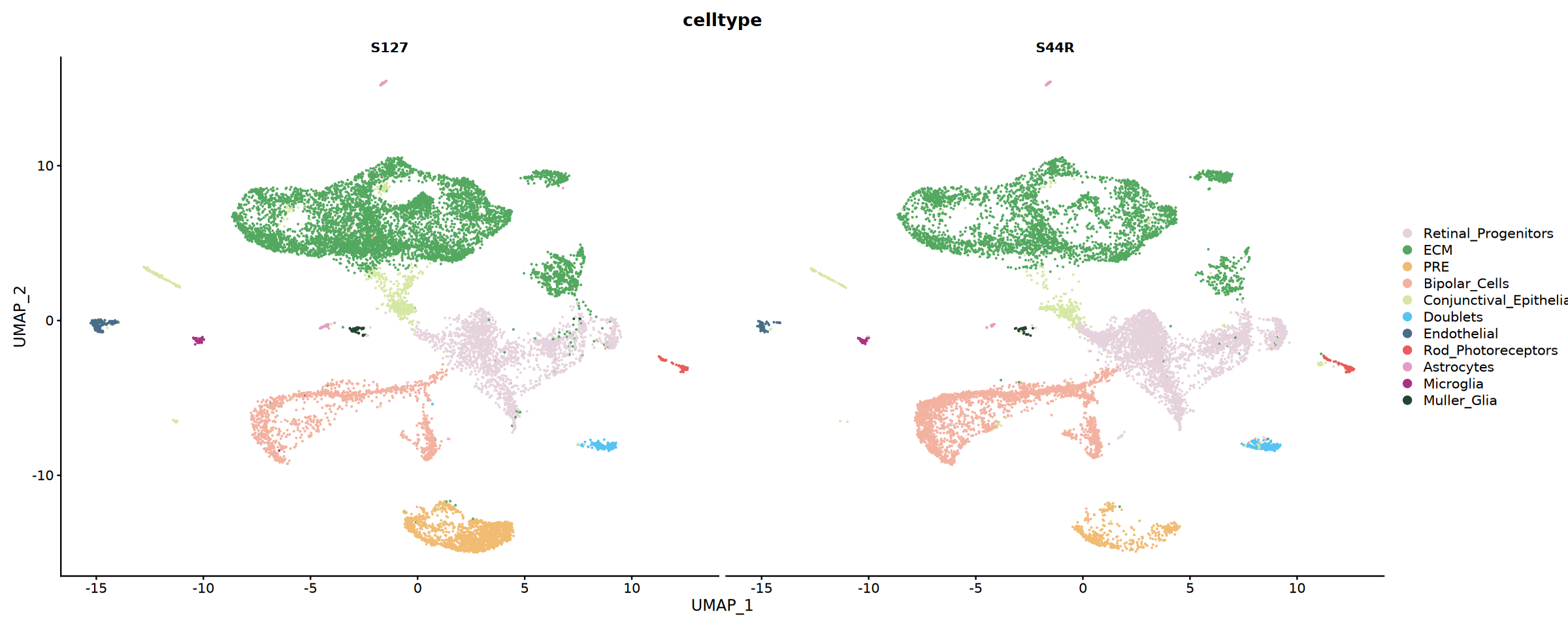
Visualize annotations by coloring UMAP or faceting by sample; calculate sample proportions for cell types for comparison.

options(repr.plot.width = 10, repr.plot.height = 8)
# Cell Type UMAP Visualization
p1 <- DimPlot(
  obj_integrated,
  reduction = "umap",
  group.by = "celltype",
  label = TRUE,
  label.size = 3,
  cols = my36colors
) +
  theme(legend.position = "bottom")

# Show cell type distribution by sample
p2 <- DimPlot(
  obj_integrated,
  reduction = "umap",
  group.by = "celltype",
  split.by = "Sample",
  cols = my36colors,
  ncol = 2
) 

# Save cell type annotation plot
pdf("celltype_annotation.pdf", width = 16, height = 12)
print(p1)
print(p2)
dev.off()

print(p1)
options(repr.plot.width = 20, repr.plot.height = 8)
print(p2)

pdf: 2

Save Results

Save integrated object and key plots; recommend saving intermediate objects for reproducibility and review.

# Save integrated Seurat object
saveRDS(obj_integrated, file = "scRNA_scRNA_integrated.rds")

Summary

This tutorial demonstrated the complete workflow for scRNA-seq multi-sample integration, covering:

• Data Loading: Import 10x matrix, create Seurat object
• QC: Calculate metrics and filter low-quality cells
• Preprocessing: Normalization and HVG identification
• Merging: Combine samples retaining origin info
• Integration: Use CCA/RPCA to remove batch effects
• Dim Reduction & Clustering: PCA, UMAP, and graph clustering
• Annotation: Marker-based interpretation and visualization

Best Practices:

• Dynamically adjust QC and integration parameters (thresholds, dims, anchors)
• Combine biological priors with public databases for annotation
• Save objects by stage to ensure traceability and reproducibility

Suggestions for Downstream Analysis:

• Tissue specificity analysis
• Differential enrichment analysis
• Pseudotime analysis
• Cell-cell interaction analysis

sessionInfo()

output

R version 4.3.3 (2024-02-29)
Platform: x86_64-conda-linux-gnu (64-bit)
Running under: Debian GNU/Linux 12 (bookworm)

Matrix products: default
BLAS/LAPACK: /jp_envs/envs/common/lib/libopenblasp-r0.3.29.so; LAPACK version 3.12.0

locale:
[1] LC_CTYPE=C.UTF-8 LC_NUMERIC=C LC_TIME=C.UTF-8
[4] LC_COLLATE=C.UTF-8 LC_MONETARY=C.UTF-8 LC_MESSAGES=C.UTF-8
[7] LC_PAPER=C.UTF-8 LC_NAME=C LC_ADDRESS=C
[10] LC_TELEPHONE=C LC_MEASUREMENT=C.UTF-8 LC_IDENTIFICATION=C

time zone: Asia/Shanghai
tzcode source: system (glibc)

attached base packages:
[1] stats graphics grDevices utils datasets methods base

other attached packages:
[1] future_1.40.0 harmony_1.2.3 Rcpp_1.0.14 patchwork_1.3.0
[5] ggplot2_3.5.2 dplyr_1.1.4 SeuratObject_4.1.4 Seurat_4.4.0
[9] repr_1.1.7

loaded via a namespace (and not attached):
[1] deldir_2.0-4 pbapply_1.7-2 gridExtra_2.3
[4] rlang_1.1.5 magrittr_2.0.3 RcppAnnoy_0.0.22
[7] spatstat.geom_3.3-6 matrixStats_1.5.0 ggridges_0.5.6
[10] compiler_4.3.3 png_0.1-8 vctrs_0.6.5
[13] reshape2_1.4.4 stringr_1.5.1 pkgconfig_2.0.3
[16] crayon_1.5.3 fastmap_1.2.0 labeling_0.4.3
[19] promises_1.3.2 ggbeeswarm_0.7.2 purrr_1.0.4
[22] jsonlite_2.0.0 goftest_1.2-3 later_1.4.2
[25] uuid_1.2-1 spatstat.utils_3.1-3 irlba_2.3.5.1
[28] parallel_4.3.3 cluster_2.1.8.1 R6_2.6.1
[31] ica_1.0-3 stringi_1.8.7 RColorBrewer_1.1-3
[34] spatstat.data_3.1-6 reticulate_1.42.0 parallelly_1.43.0
[37] spatstat.univar_3.1-2 lmtest_0.9-40 scattermore_1.2
[40] IRkernel_1.3.2 tensor_1.5 future.apply_1.11.3
[43] zoo_1.8-14 R.utils_2.13.0 base64enc_0.1-3
[46] sctransform_0.4.1 httpuv_1.6.15 Matrix_1.6-5
[49] splines_4.3.3 igraph_2.0.3 tidyselect_1.2.1
[52] abind_1.4-5 spatstat.random_3.3-3 codetools_0.2-20
[55] miniUI_0.1.1.1 spatstat.explore_3.4-2 listenv_0.9.1
[58] lattice_0.22-7 tibble_3.2.1 plyr_1.8.9
[61] withr_3.0.2 shiny_1.10.0 ROCR_1.0-11
[64] ggrastr_1.0.2 evaluate_1.0.3 Rtsne_0.17
[67] survival_3.8-3 polyclip_1.10-7 fitdistrplus_1.2-2
[70] pillar_1.10.2 KernSmooth_2.23-26 plotly_4.10.4
[73] generics_0.1.3 sp_2.2-0 IRdisplay_1.1
[76] munsell_0.5.1 scales_1.3.0 globals_0.16.3
[79] xtable_1.8-4 glue_1.8.0 lazyeval_0.2.2
[82] tools_4.3.3 data.table_1.17.0 pbdZMQ_0.3-13
[85] RANN_2.6.2 leiden_0.4.3.1 Cairo_1.6-2
[88] cowplot_1.1.3 grid_4.3.3 tidyr_1.3.1
[91] colorspace_2.1-1 nlme_3.1-168 beeswarm_0.4.0
[94] vipor_0.4.7 cli_3.6.4 spatstat.sparse_3.1-0
[97] viridisLite_0.4.2 uwot_0.2.3 gtable_0.3.6
[100] R.methodsS3_1.8.2 digest_0.6.37 progressr_0.15.1
[103] ggrepel_0.9.6 htmlwidgets_1.6.4 farver_2.1.2
[106] R.oo_1.27.0 htmltools_0.5.8.1 lifecycle_1.0.4
[109] httr_1.4.7 mime_0.13 MASS_7.3-60.0.1