SeekArc Single-Cell Multi-Omics (RNA+ATAC) Single Sample Analysis Tutorial (WNN)

Author: SeekGene

Time: 19 min

Words: 3.7k words

Updated: 2026-02-28

Reads: 0 times

scATAC + RNA-seq Analysis Guide Notebooks Basic Analysis

Environment Preparation

Load R Packages

Please select the common_r environment for this integration tutorial

# Load necessary R packages
suppressPackageStartupMessages({
  library(Seurat)
  library(Signac)
  library(EnsDb.Hsapiens.v86, lib.loc = "/PROJ2/FLOAT/shumeng/apps/miniconda3/envs/python3.10/lib/R/library")
  library(BSgenome.Hsapiens.UCSC.hg38,lib = "/PROJ2/FLOAT/shumeng/apps/miniconda3/envs/python3.10/lib/R/library")
  library(biovizBase, lib = "/PROJ2/FLOAT/shumeng/apps/miniconda3/envs/python3.10/lib/R/library")
  #library(BSgenome.Mmusculus.UCSC.mm10)
  #library(EnsDb.Mmusculus.v79)
  library(dplyr)
  library(ggplot2)
  library(patchwork)
  library(harmony)
})

# Set random seed
set.seed(1234)

# Set Seurat options (Note: 8000 * 1024^2 is actually 8GB)
options(future.globals.maxSize = 8000 * 1024^2)  # 8GB

# Define color scheme
my36colors <-c( '#E5D2DD', '#53A85F', '#F1BB72', '#F3B1A0', '#D6E7A3', '#57C3F3', '#476D87',
                '#E95C59', '#E59CC4', '#AB3282', '#23452F', '#BD956A', '#8C549C', '#585658',
                '#9FA3A8', '#E0D4CA', '#5F3D69', '#C5DEBA', '#58A4C3', '#E4C755', '#F7F398',
                '#AA9A59', '#E63863', '#E39A35', '#C1E6F3', '#6778AE', '#91D0BE', '#B53E2B',
                '#712820', '#DCC1DD', '#CCE0F5', '#CCC9E6', '#625D9E', '#68A180', '#3A6963',
                '#968175', "#6495ED", "#FFC1C1",'#f1ac9d','#f06966','#dee2d1','#6abe83','#39BAE8','#B9EDF8','#221a12',
                '#b8d00a','#74828F','#96C0CE','#E95D22','#017890')

Get Gene Annotation Information

We will obtain genome annotation information (gene positions, transcripts, exons, TSS, etc.) for the corresponding species from the EnsDb database. The specific species needs to be changed according to the data. This information is used for:

• Calculating ATAC TSS enrichment (determining if open chromatin is more concentrated near transcription start sites)
• Constructing gene activity matrix (mapping peak signals to genes)
• Peak annotation and functional analysis

Notes:

• Species must match reference genome version (e.g., EnsDb.Hsapiens.v86 for hg38, EnsDb.Mmusculus.v75 for mm10)
• Consistent chromosome naming style (e.g., using prefixes like chr1, chr2)

# Get gene annotation information (silence warnings and messages)
suppressWarnings({
  suppressMessages({
    annotation <- GetGRangesFromEnsDb(ensdb = EnsDb.Hsapiens.v86)
    seqlevels(annotation) <- paste0('chr', seqlevels(annotation))
    genome(annotation) <- 'hg38'
  })
})

Data Reading

This tutorial provides two different data input methods to meet different user data acquisition needs. Choose the one that suits you:

Cloud Platform RDS File Reading

Data Characteristics:

• RDS file is a standard Seurat object file
• Can be directly used for subsequent downstream analysis, or expression matrix can be extracted for re-integration

Applicable Scenarios:

• When you cannot obtain the standard filtered_feature_bc_matrix expression matrix
• When you want to use existing data on the cloud platform for learning
• When you need to quickly re-perform basic analysis

Notes:

• For specific data mounting and RDS file reading, please refer to the Jupyter usage tutorial

For example, the following project data /home/demo-SeekGene-com/workspace/data/AY1752565399550/

# For example, the following project data /home/demo-seekgene-com/workspace/data/AY1752565399550/
#input <- readRDS("/home/demo-seekgene-com/workspace/data/AY1752565399550/input.rds")
#meta <- read.table("/home/demo-seekgene-com/workspace/data/AY1752565399550/meta.tsv", header=TRUE, sep="\t", row.names = 1)


# Extract genome annotation file from original RDS data
#annotations <- Annotation(input)
#seu <- CreateSeuratObject(counts = input@assay$RNA@counts, meta.data=meta)
#seu[["ATAC"]] <- CreateChromatinAssay(seu, counts = input@assay$ATAC@counts, fragments = input@assay$ATAC@fragments)
#Annotation(seu) <- annotations
#rm(input)
#gc()

Standard filtered_XXXX_bc_matrix File Reading

Applicable Scenarios:

• When you have standard gene expression matrix and peaks open matrix files
• When you want to independently complete basic analysis of single-cell multi-omics (SeekArc) data
• When you need a complete workflow from raw data to analysis results

Note:

• Please ensure the file structure is as follows:

The data directory structure must meet the following requirements:

1. The sample folder name is the sample ID, such as S127.
2. The sample folder contains the following files:
   • filtered_feature_bc_matrix: scRNA-seq expression matrix folder, containing barcodes.tsv.gz, features.tsv.gz, and matrix.mtx.gz files.
   • filtered_peaks_bc_matrix: ATAC peak open matrix folder, containing barcodes.tsv.gz, features.tsv.gz, and matrix.mtx.gz files.
   • {Sample ID}_A_fragments.tsv.gz: ATAC fragments file, such as S127_A_fragments.tsv.gz.
   • {Sample ID}_A_fragments.tsv.gz.tbi: ATAC fragments index file, such as S127_A_fragments.tsv.gz.tbi.

The specific folder structure is as follows:

├── S127/
│ ├── filtered_feature_bc_matrix/ (scRNA-seq expression matrix)
│ │ ├── barcodes.tsv.gz
│ │ ├── features.tsv.gz
│ │ └── matrix.mtx.gz
│ ├── filtered_peaks_bc_matrix/ (ATAC peak open matrix)
│ │ ├── barcodes.tsv.gz
│ │ ├── features.tsv.gz
│ │ └── matrix.mtx.gz
│ ├── S127_A_fragments.tsv.gz (ATAC fragments file)
│ └── S127_A_fragments.tsv.gz.tbi

# load the RNA and ATAC data
RNA_counts <- Read10X("./S127/filtered_feature_bc_matrix/")
ATAC_counts <- Read10X("./S127/filtered_peaks_bc_matrix/")
fragpath <- "./S127/S127_A_fragments.tsv.gz"

# create a Seurat object containing the RNA adata
seu <- CreateSeuratObject(
  counts = RNA_counts,
  assay = "RNA"
)

# create ATAC assay and add it to the object
seu[["ATAC"]] <- CreateChromatinAssay(
  counts = ATAC_counts,
  sep = c(":", "-"),
  fragments = fragpath,
  annotation = annotation
)

output

Computing hash

Data Quality Control

Calculation of Quality Control Metrics

RNA QC Metrics:

• percent.mt: Percentage of mitochondrial genes (usually <20%)
• nfeature_RNA: Number of RNA features (usually between 200-10000)

ATAC QC Metrics:

• TSS.enrichment: TSS enrichment score (usually >2)
• nucleosome_signal: Nucleosome signal (lower is better)
• nCount_ATAC: Total ATAC count (usually between 1000-10000)

# Perform quality control for each sample
suppressWarnings({
  suppressMessages({
          # RNA QC metrics
          seu[["percent.mt"]] <- PercentageFeatureSet(seu, pattern = "^MT-")
          # ATAC QC metrics
          DefaultAssay(seu) <- "ATAC"
          # Calculate TSS enrichment score
          seu <- TSSEnrichment(object = seu, fast = FALSE) 
          # Calculate nucleosome signal
          seu <- NucleosomeSignal(object = seu)
  })
})

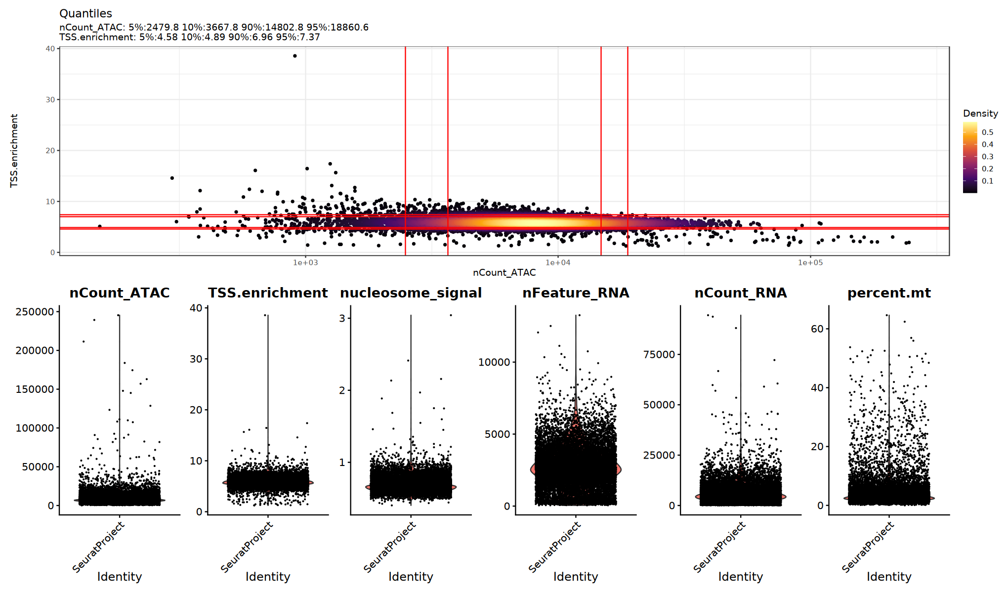
Visualization of Quality Control Metrics

Use violin plots to view the distribution/outliers of QC metrics and determine appropriate thresholds:

Suggestions:

• Observe if there are obvious long tails or bimodal distributions
• Try multiple sets of thresholds and compare if downstream clustering/UMAP is clearer

# Visualize QC metrics. This cell is optional.
options(repr.plot.width = 17, repr.plot.height = 10)
suppressWarnings({
  p1=DensityScatter(seu, x = 'nCount_ATAC', y = 'TSS.enrichment', log_x = TRUE, quantiles = TRUE)
  p2=VlnPlot(
      object = seu,
      features = c('nCount_ATAC', 'TSS.enrichment',  'nucleosome_signal',"nFeature_RNA", "nCount_RNA", "percent.mt"),
      pt.size = 0.1,
      ncol = 6
  )
 print(p1 / p2)
})

Filtering Low Quality Cells

Filter low quality cells based on QC metrics. Specific thresholds should be adjusted according to data characteristics and violin plot distributions.

# Quality Control Filtering
 
cells_before <- ncol(seu)
  
seu <- subset(seu,
    subset = nFeature_RNA > 200 &
             nFeature_RNA < 8000 &
             nCount_RNA > 500 &
             nCount_RNA < 30000 &
             percent.mt < 20 &
             nCount_ATAC > 500 &
             nCount_ATAC < 100000 &
             TSS.enrichment > 1 &
             nucleosome_signal < 2
  )
  
  cells_after <- ncol(seu)

Data Normalization

RNA Data Normalization and Linear Dimensionality Reduction

Normalization Method: By default, Seurat uses "LogNormalize" global scaling normalization method:

• First normalizes feature expression for each cell by total expression
• Multiplies by a scale factor (default is 10,000)
• Then log-transforms the result

Feature Selection: Identifies a subset of features that exhibit high cell-to-cell variation in the dataset (i.e., they are highly expressed in some cells, and lowly expressed in others)

Data Scaling: Applies a linear transformation ("scaling"), a standard pre-processing step prior to dimensional reduction techniques like PCA

Dimensionality Reduction: Perform PCA on the normalized data

suppressWarnings({
  suppressMessages({
      DefaultAssay(seu) <- "RNA"
      seu <- NormalizeData(seu, assay = "RNA")
      seu <- FindVariableFeatures(seu, assay = "RNA", selection.method = "vst", nfeatures = 2000)
      seu <- ScaleData(seu, assay = "RNA")
      seu <- RunPCA(seu, assay = "RNA", npcs = 50)
      })
    })

ATAC Data Normalization and Linear Dimensionality Reduction

Normalization Method: Signac uses Term Frequency-Inverse Document Frequency (TF-IDF) normalization:

• Normalizes across cells to correct for sequencing depth differences
• Normalizes across peaks to give higher weight to rare peaks

Feature Selection Strategy: Due to the low dynamic range of scATAC-seq data, we cannot perform variable feature selection like in scRNA-seq. Alternatively, we can use FindTopFeatures() to select top n% features (peaks) or remove features present in fewer than n cells.

Dimensionality Reduction: Then perform Singular Value Decomposition (SVD) on the TF-IDF matrix using the selected features.

suppressWarnings({
  suppressMessages({
      seu <- RunTFIDF(seu, assay = "ATAC")
      seu <- FindTopFeatures(seu, assay = "ATAC", min.cutoff = 'q0')
      seu <- RunSVD(seu, assay = "ATAC")
  })
})

Non-linear Dimensionality Reduction and Clustering

Three Clustering Strategies

1. RNA Clustering: Based on gene expression similarity
2. ATAC Clustering: Based on chromatin accessibility similarity
3. WNN Clustering: Integrating both modalities (Recommended)

Result Interpretation

• Different methods may produce different clustering results
• WNN clustering usually reveals more detailed cell subpopulations
• It is recommended to prioritize WNN results for downstream analysis

RNA Dimensionality Reduction and Clustering

RNA Clustering Strategy:

• Independent clustering analysis based on RNA data
• Classifying cells using gene expression patterns

suppressWarnings({
  suppressMessages({
      seu <- RunUMAP(seu, reduction = "pca", dims = 1:30, assay = "RNA",reduction.name="rnaumap")
      seu <- FindNeighbors(seu, reduction = "pca", dims = 1:30, assay = "RNA",graph.name = "rnaneigobr")
      seu <- FindClusters(seu, resolution = 0.5, algorithm = 1,graph.name = "rnaneigobr")
        })
})

output

Modularity Optimizer version 1.3.0 by Ludo Waltman and Nees Jan van Eck

Number of nodes: 12694
Number of edges: 119839

Running Louvain algorithm...n Maximum modularity in 10 random starts: 0.9108
Number of communities: 25
Elapsed time: 0 seconds

ATAC Dimensionality Reduction and Clustering

ATAC Clustering Strategy:

• Independent clustering analysis based on ATAC data
• Classifying cells using chromatin accessibility patterns

suppressWarnings({
  suppressMessages({
      seu <- RunUMAP(seu, reduction = "lsi", dims = 1:30, assay = "ATAC",reduction.name="atacumap")
      seu <- FindNeighbors(seu, reduction = "lsi", dims = 1:30, assay = "ATAC",graph.name = "atacneigobr")
      seu <- FindClusters(seu, resolution = 0.5, algorithm = 1,graph.name = "atacneigobr")
        })
})

output

Modularity Optimizer version 1.3.0 by Ludo Waltman and Nees Jan van Eck

Number of nodes: 12694
Number of edges: 120530

Running Louvain algorithm...n Maximum modularity in 10 random starts: 0.8927
Number of communities: 19
Elapsed time: 0 seconds

Weighted Nearest Neighbor (WNN) Analysis

WNN Integrated Clustering Strategy:

• Weighted nearest neighbor analysis combining RNA and ATAC data
• Provides more accurate cell type identification

suppressWarnings({
  suppressMessages({
      seu <- FindMultiModalNeighbors(seu, reduction.list = list("pca", "lsi"), dims.list = list(1:30, 1:30))
      # Clustering based on WNN
      seu <- FindClusters(seu, graph.name = "wknn", resolution = 0.5)
      # WNN UMAP
      seu <- RunUMAP(seu, nn.name = "weighted.nn", reduction.name = "wnn.umap")
        })
})

output

Modularity Optimizer version 1.3.0 by Ludo Waltman and Nees Jan van Eck

Number of nodes: 12694
Number of edges: 191058

Running Louvain algorithm...n Maximum modularity in 10 random starts: 0.8993
Number of communities: 20
Elapsed time: 0 seconds

Visualization

# Compare clustering results of different methods
p1 <- DimPlot(seu, reduction = "rnaumap", group.by = "rnaneigobr_res.0.5",label=T, cols = my36colors) + ggtitle("RNA")
p2 <- DimPlot(seu, reduction = "atacumap", group.by = "atacneigobr_res.0.5",label=T, cols = my36colors) + ggtitle("ATAC")
p3 <- DimPlot(seu, reduction = "wnn.umap", group.by = "wknn_res.0.5",label=T, cols = my36colors) + ggtitle("WNN")

options(repr.plot.width=23, repr.plot.height=6)
print(p1 + p2 + p3)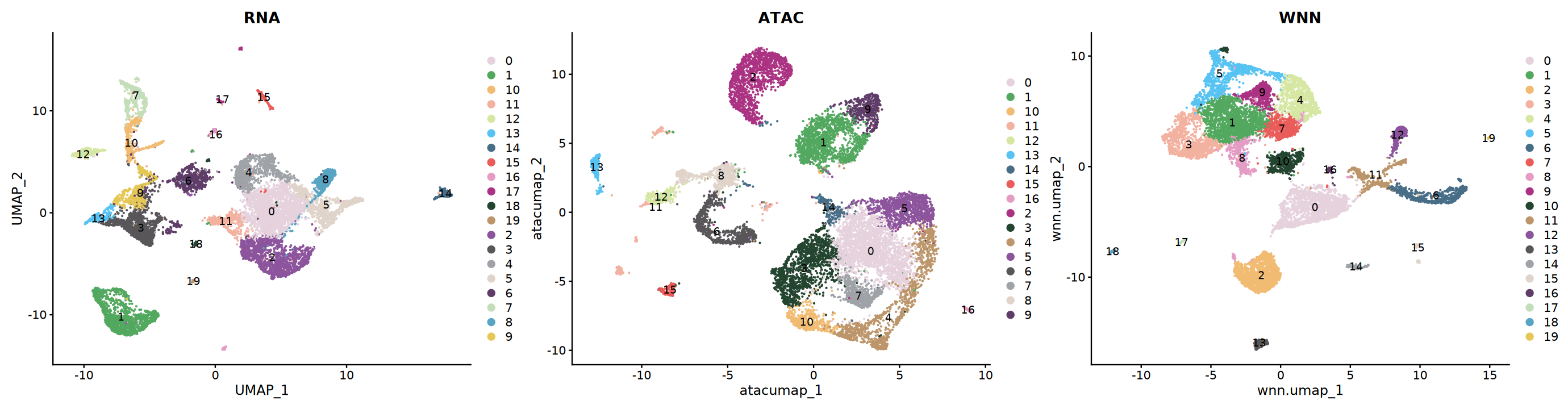

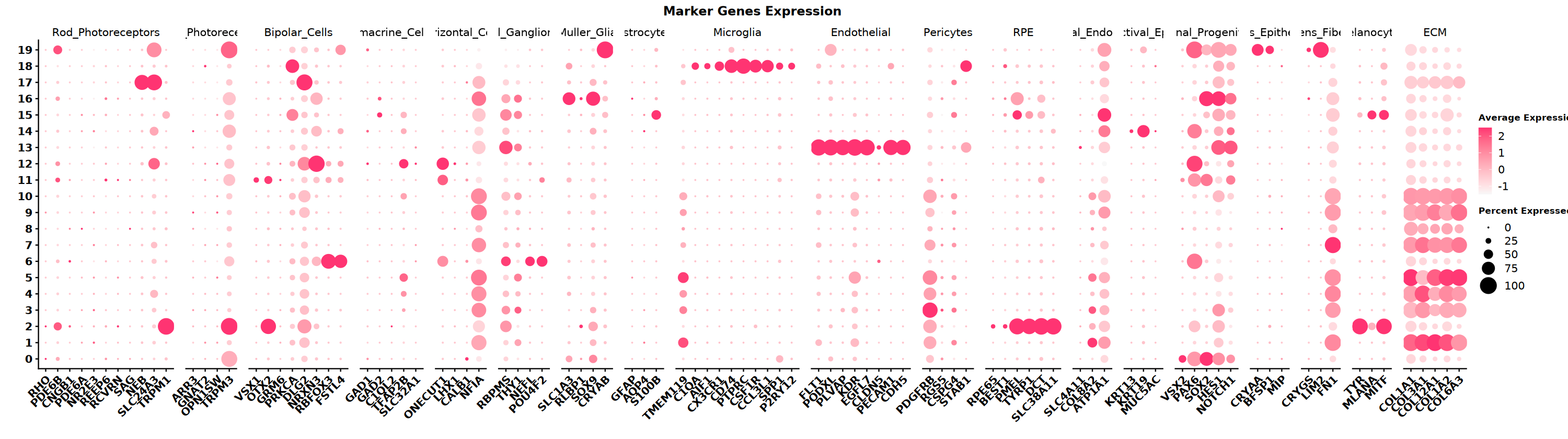
Cell Type Annotation

Marker Genes

Collect marker gene sets for different cell types based on tissue type. This example data is from the eye. Below are cell types in the eye and their corresponding marker genes. Use dot plots to visualize which cell type markers are highly expressed in different clusters.

eye_marker_integrated <- list(
  # ========== Photoreceptor Cells ==========
  "Rod_Photoreceptors" = c("RHO", "PDE6B", "CNGB1", "PDE6A", "NR2E3", "REEP6",
                          "RCVRN", "SAG", "NEB", "SLC24A3", "TRPM1"),
  "Cone_Photoreceptors" = c("ARR3", "GNAT2", "OPN1SW", "TRPM3"),

  # ========== Retinal Neurons ==========
  "Bipolar_Cells" = c("VSX1", "OTX2", "GRM6", "PRKCA",
                     "DLG2", "NRXN3", "RBFOX3", "FSTL4"),
  "Amacrine_Cells" = c("GAD1", "GAD2", "C1QL2", "TFAP2B", "SLC32A1"),
  "Horizontal_Cells" = c("ONECUT1", "LHX1", "CALB1", "NFIA"),
  "Retinal_Ganglion_Cells" = c("RBPMS", "THY1", "NEFL", "POU4F2"),

  # ========== Glial Cells ==========
  "Muller_Glia" = c("SLC1A3", "RLBP1", "SOX9", "CRYAB"),
  "Astrocytes" = c("GFAP", "AQP4", "S100B"),
  "Microglia" = c("TMEM119", "C1QA", "AIF1", "CX3CR1", "CD74",
                 "PTPRC", "CSF1R", "CCL3L1", "SPP1", "P2RY12"),

  # ========== Vascular and Support Cells ==========
  "Endothelial" = c("FLT1", "PODXL", "PLVAP", "KDR", "EGFL7",
                   "CLDN5", "PECAM1", "CDH5"),
  "Pericytes" = c("PDGFRB", "RGS5", "CSPG4", "STAB1"),

  # ========== Epithelial Cells ==========
  "RPE" = c("RPE65", "BEST1", "PMEL", "TYRP1", "DCT", "SLC38A11"),
  #"Corneal_Epithelial" = c("KRT12", "KRT3"),
  "Corneal_Endothelial" = c("SLC4A11", "COL8A2", "ATP1A1"),
  "Conjunctival_Epithelial" = c("KRT13", "KRT19", "MUC5AC"),
  "Retinal_Progenitors" = c("VSX2", "PAX6","SOX2", "HES1", "NOTCH1"),  # Neural retina proliferation stage

  # ========== Lens Cells ==========
  "Lens_Epithelial" = c("CRYAA", "BFSP1", "MIP"),
  "Lens_Fiber" = c("CRYGS", "LIM2", "FN1"),

  # ========== Other Cells ==========
  "Melanocytes" = c("TYR", "MLANA", "MITF"),
  #"Erythrocytes" = c("HBB", "HBA1", "HBA2"),
  "ECM" = c("COL1A1", "COL3A1", "COL12A1", "COL1A2", "COL6A3")#,
  #"Others" = c("TTN", "CLCN5", "DCC", "MIAT")
)

# Set plot size
options(repr.plot.width=25, repr.plot.height=7)

# Draw DotPlot
DefaultAssay(seu)="RNA"
DotPlot(seu, 
        group.by = "wknn_res.0.5", 
        features = eye_marker_integrated,
        cols = c("#f8f8f8","#ff3472"),
       #dot.min = 0.05,
       dot.scale = 8)+  # Apply custom colors
  RotatedAxis() + 
  scale_x_discrete("") + 
  scale_y_discrete("") +
  theme(
    axis.text.x = element_text(size = 12, face = "bold", 
                              angle = 45, hjust = 1, vjust = 1),
    axis.text.y = element_text(size = 12, face = "bold"),
    plot.title = element_text(size = 14, face = "bold", hjust = 0.5),
    legend.title = element_text(size = 10, face = "bold")
  ) +
  ggtitle("Marker Genes Expression") +
  labs(color = "Expression\nLevel")  # Modify legend title

output

Warning message:
"The \`facets\` argument of \`facet_grid()\` is deprecated as of ggplot2 2.2.0.
ℹ Please use the \`rows\` argument instead.
ℹ The deprecated feature was likely used in the Seurat package.
Please report the issue at ."

** Notes ** SeekArc single-cell dual-omics cell annotation is generally based on WNN multimodal dimensionality reduction, annotating based on marker gene expression in wknn clustering results

options(repr.plot.width=10, repr.plot.height=8)
DimPlot(seu, reduction = "wnn.umap", group.by = "wknn_res.0.5", cols = my36colors,label = T)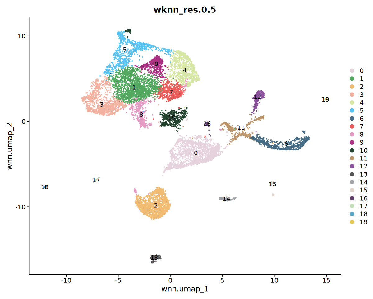

Cell Type Labeling

cat('Starting cell type annotation...', Sys.time(), '\n')

# Cell type annotation based on clustering results (adjust according to actual marker gene expression)
# Here is an example, adjust according to DotPlot results in actual use
celltype_mapping <- c(
  "0" = "Retinal_Progenitors",
  "1" = "ECM",
  "2" = "PRE",
  "3" = "ECM",
  "4" = "ECM",
  "5" = "ECM",
  "6" = "Bipolar_Cells",
  "7" = "ECM",
  "8" = "ECM",
  "9" = "ECM",
  "10" = "ECM",
  "11" = "Bipolar_Cells",
  "12" = "Bipolar_Cells",
  "13" = "Endothelial",
  "14" = "Conjunctival_Epithelial",
  "15" = "Astrocytes",
  "16" = "Muller_Glia",
  "17" = "Rod_Photoreceptors",
  "18" = "Microglia",
  "19" = "Lens"
)

# Apply cell type annotation
seu$celltype <- recode(
  seu$wknn_res.0.5,
  !!!celltype_mapping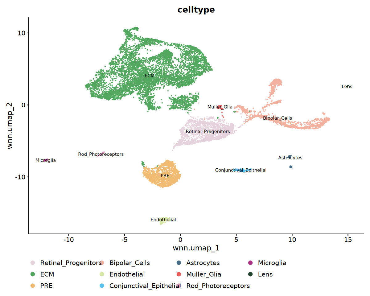
)

output

开始细胞类型注释... 1755579264

Visualization of Annotation Results

cat('Visualizing cell type annotation...', '\n')

# Cell type UMAP visualization
p1 <- DimPlot(
  seu,
  reduction = "wnn.umap",
  group.by = "celltype",
  label = TRUE,
  label.size = 3,
  cols = my36colors
) +
  ggtitle("celltype") +
  theme(legend.position = "bottom")

# Save cell type annotation plot
pdf("celltype_annotation.pdf", width = 16, height = 12)
print(p1)
dev.off()
options(repr.plot.width=10, repr.plot.height=8)
print(p1)

output

细胞类型注释可视化...

pdf: 2

Save Results

# Save integrated Seurat object
saveRDS(seu, file = "processed.rds")

Summary

This tutorial demonstrated the single-sample analysis workflow for single-cell multi-omics data.

Future Analysis Directions

• Cell type annotation and marker gene identification
• Differential expression and differential accessibility analysis
• Co-accessibility analysis of genes and peaks
• Motif analysis
• Footprint analysis
• Gene regulatory network inference
• Trajectory and pseudotime analysis
• CNV analysis
• Joint analysis of epigenetic traits and ATAC

sessionInfo()

output

R version 4.3.3 (2024-02-29)
Platform: x86_64-conda-linux-gnu (64-bit)
Running under: Debian GNU/Linux 12 (bookworm)

Matrix products: default
BLAS/LAPACK: /jp_envs/envs/common/lib/libopenblasp-r0.3.29.so; LAPACK version 3.12.0

locale:
[1] LC_CTYPE=C.UTF-8 LC_NUMERIC=C LC_TIME=C.UTF-8
[4] LC_COLLATE=C.UTF-8 LC_MONETARY=C.UTF-8 LC_MESSAGES=C.UTF-8
[7] LC_PAPER=C.UTF-8 LC_NAME=C LC_ADDRESS=C
[10] LC_TELEPHONE=C LC_MEASUREMENT=C.UTF-8 LC_IDENTIFICATION=C

time zone: Asia/Shanghai
tzcode source: system (glibc)

attached base packages:
[1] stats4 stats graphics grDevices utils datasets methods
[8] base

other attached packages:
[1] future_1.40.0 harmony_1.2.3
[3] Rcpp_1.0.14 patchwork_1.3.0
[5] ggplot2_3.5.2 dplyr_1.1.4
[7] biovizBase_1.50.0 BSgenome.Hsapiens.UCSC.hg38_1.4.5
[9] BSgenome_1.70.1 rtracklayer_1.62.0
[11] BiocIO_1.12.0 Biostrings_2.70.1
[13] XVector_0.42.0 EnsDb.Hsapiens.v86_2.99.0
[15] ensembldb_2.26.0 AnnotationFilter_1.26.0
[17] GenomicFeatures_1.54.1 AnnotationDbi_1.64.1
[19] Biobase_2.62.0 GenomicRanges_1.54.1
[21] GenomeInfoDb_1.38.1 IRanges_2.36.0
[23] S4Vectors_0.40.2 BiocGenerics_0.48.1
[25] Signac_1.10.0 SeuratObject_4.1.4
[27] Seurat_4.4.0

loaded via a namespace (and not attached):
[1] ProtGenerics_1.34.0 matrixStats_1.5.0
[3] spatstat.sparse_3.1-0 bitops_1.0-9
[5] httr_1.4.7 RColorBrewer_1.1-3
[7] repr_1.1.7 tools_4.3.3
[9] sctransform_0.4.1 backports_1.5.0
[11] R6_2.6.1 lazyeval_0.2.2
[13] uwot_0.2.3 withr_3.0.2
[15] sp_2.2-0 prettyunits_1.2.0
[17] gridExtra_2.3 progressr_0.15.1
[19] cli_3.6.4 Cairo_1.6-2
[21] spatstat.explore_3.4-2 labeling_0.4.3
[23] spatstat.data_3.1-6 ggridges_0.5.6
[25] pbapply_1.7-2 Rsamtools_2.18.0
[27] pbdZMQ_0.3-13 foreign_0.8-87
[29] R.utils_2.13.0 dichromat_2.0-0.1
[31] parallelly_1.43.0 rstudioapi_0.15.0
[33] RSQLite_2.3.9 generics_0.1.3
[35] ica_1.0-3 spatstat.random_3.3-3
[37] Matrix_1.6-5 ggbeeswarm_0.7.2
[39] abind_1.4-5 R.methodsS3_1.8.2
[41] lifecycle_1.0.4 yaml_2.3.10
[43] SummarizedExperiment_1.32.0 SparseArray_1.2.2
[45] BiocFileCache_2.10.1 Rtsne_0.17
[47] grid_4.3.3 blob_1.2.4
[49] promises_1.3.2 crayon_1.5.3
[51] miniUI_0.1.1.1 lattice_0.22-7
[53] cowplot_1.1.3 KEGGREST_1.42.0
[55] pillar_1.10.2 knitr_1.49
[57] rjson_0.2.23 future.apply_1.11.3
[59] codetools_0.2-20 fastmatch_1.1-6
[61] leiden_0.4.3.1 glue_1.8.0
[63] spatstat.univar_3.1-2 data.table_1.17.0
[65] vctrs_0.6.5 png_0.1-8
[67] gtable_0.3.6 cachem_1.1.0
[69] xfun_0.50 S4Arrays_1.2.0
[71] mime_0.13 survival_3.8-3
[73] RcppRoll_0.3.1 fitdistrplus_1.2-2
[75] ROCR_1.0-11 nlme_3.1-168
[77] bit64_4.5.2 progress_1.2.3
[79] filelock_1.0.3 RcppAnnoy_0.0.22
[81] irlba_2.3.5.1 vipor_0.4.7
[83] KernSmooth_2.23-26 rpart_4.1.23
[85] colorspace_2.1-1 DBI_1.2.3
[87] Hmisc_5.2-1 nnet_7.3-19
[89] ggrastr_1.0.2 tidyselect_1.2.1
[91] bit_4.5.0.1 compiler_4.3.3
[93] curl_6.0.1 htmlTable_2.4.3
[95] xml2_1.3.6 DelayedArray_0.28.0
[97] plotly_4.10.4 checkmate_2.3.2
[99] scales_1.3.0 lmtest_0.9-40
[101] rappdirs_0.3.3 stringr_1.5.1
[103] digest_0.6.37 goftest_1.2-3
[105] spatstat.utils_3.1-3 rmarkdown_2.29
[107] htmltools_0.5.8.1 pkgconfig_2.0.3
[109] base64enc_0.1-3 MatrixGenerics_1.14.0
[111] dbplyr_2.5.0 fastmap_1.2.0
[113] rlang_1.1.5 htmlwidgets_1.6.4
[115] shiny_1.10.0 farver_2.1.2
[117] zoo_1.8-14 jsonlite_2.0.0
[119] BiocParallel_1.36.0 R.oo_1.27.0
[121] VariantAnnotation_1.48.1 RCurl_1.98-1.16
[123] magrittr_2.0.3 Formula_1.2-5
[125] GenomeInfoDbData_1.2.11 IRkernel_1.3.2
[127] munsell_0.5.1 reticulate_1.42.0
[129] stringi_1.8.7 zlibbioc_1.48.0
[131] MASS_7.3-60.0.1 plyr_1.8.9
[133] parallel_4.3.3 listenv_0.9.1
[135] ggrepel_0.9.6 deldir_2.0-4
[137] IRdisplay_1.1 splines_4.3.3
[139] tensor_1.5 hms_1.1.3
[141] igraph_2.0.3 uuid_1.2-1
[143] spatstat.geom_3.3-6 reshape2_1.4.4
[145] biomaRt_2.58.0 XML_3.99-0.17
[147] evaluate_1.0.3 httpuv_1.6.15
[149] RANN_2.6.2 tidyr_1.3.1
[151] purrr_1.0.4 polyclip_1.10-7
[153] scattermore_1.2 xtable_1.8-4
[155] restfulr_0.0.15 later_1.4.2
[157] viridisLite_0.4.2 tibble_3.2.1
[159] memoise_2.0.1 beeswarm_0.4.0
[161] GenomicAlignments_1.38.0 cluster_2.1.8.1
[163] globals_0.16.3