SeekSpace Spatial Transcriptomics Data Analysis Tutorial (Scanpy / Mouse Brain)

Author: SeekGene

Time: 9 min

Words: 1.6k words

Updated: 2026-02-28

Reads: 0 times

Spatial-seq Analysis Guide Notebooks Basic Analysis

Background Information

This document explains the data obtained from SeekGene SeekSpace technology and its analysis method using Scanpy.
SeekGene SeekSpace technology can detect gene expression data at single-cell resolution while also locating the spatial coordinates of each cell within the tissue.
Data analysis for SeekSpace is straightforward and compatible with common single-cell transcriptomics analysis software such as Seurat and Scanpy.
This data is spatial data of a mouse brain based on SeekSpace technology. It contains a single-cell transcriptome matrix of 32,758 cells, a spatial coordinate matrix, tissue DAPI staining images, and H&E images.

File Description

The companion basic data processing software for SeekSpace technology is SeekSpace® Tools, which identifies cell expression information from sequencing libraries and locates the spatial position of each cell.
The result file format obtained after processing with SeekSpace® Tools software is as follows:

├── WTH1092_filtered_feature_bc_matrix # Expression matrix directory, can be read using Seurat's Read10X command
│ ├── barcodes.tsv.gz
│ ├── features.tsv.gz
│ ├── matrix.mtx.gz
│ └── cell_locations.tsv.gz Spatial coordinate file for cells in mouse brain sequencing data. Column 1 is the barcode, consistent with the order in filtered_feature_bc_matrix/barcode; Columns 2 and 3 are the spatial positions (pixel coordinates on the spatial chip) of the cell represented by the barcode.

├── WTH1092_aligned_DAPI.png # DAPI staining image of mouse brain tissue section
├── WTH1092_aligned_HE.png
├── WTH1092_aligned_HE_TIMG.png
├── seekspace_of_Seurat.ipynb # Jupyter example file for analyzing this mouse brain spatial data using Seurat
└── seekspace_of_scanpy.ipynb # Jupyter example file for analyzing this mouse brain spatial data using Scanpy
The size of one pixel in SeekSpace technology is approximately 0.2653 micrometers. Multiplying the pixel coordinates by 0.2653 converts them to the distance of cells in real space.

import scanpy# Core scverse libraries
import scanpy as sc
import anndata as ad
import pandas as pd
# Data retrieval
import pooch

import warnings  
warnings.filterwarnings("ignore")

sc.settings.verbosity = 3  # verbosity: errors (0), warnings (1), info (2), hints (3)
sc.logging.print_header()
sc.settings.set_figure_params(dpi=80, facecolor="white")

output

scanpy==1.9.8 anndata==0.9.2 umap==0.5.6 numpy==1.22.4 scipy==1.10.1 pandas==2.0.3 scikit-learn==1.3.2 statsmodels==0.14.1 igraph==0.9.9 pynndescent==0.5.12

Read Data Matrix

adata = sc.read_10x_mtx(
    "./Outs/WTH1092_filtered_feature_bc_matrix/",
    cache=True
)

output

... reading from cache file cache/Outs-WTH1092_filtered_feature_bc_matrix-matrix.h5ad

adata.var_names_make_unique()

adata

output

AnnData object with n_obs × n_vars = 32758 × 32285
var: 'gene_ids', 'feature_types'

Dimensionality Reduction and Clustering

## Preprocessing
adata.var["mt"] = adata.var_names.str.startswith("mt-")
sc.pp.calculate_qc_metrics(
    adata, qc_vars=["mt"], percent_top=None, log1p=False, inplace=True
)

sc.pp.normalize_total(adata, target_sum=1e4)
sc.pp.log1p(adata)
sc.pp.highly_variable_genes(adata, min_mean=0.0125, max_mean=3, min_disp=0.5)

adata.raw = adata
adata = adata[:, adata.var.highly_variable]
sc.pp.regress_out(adata, ["total_counts", "pct_counts_mt"])
sc.pp.scale(adata, max_value=10)

output

normalizing counts per cell
finished (0:00:00)
extracting highly variable genes
finished (0:00:01)
--> added
'highly_variable', boolean vector (adata.var)
'means', float vector (adata.var)
'dispersions', float vector (adata.var)
'dispersions_norm', float vector (adata.var)
regressing out ['total_counts', 'pct_counts_mt']
sparse input is densified and may lead to high memory use
finished (0:02:49)

## Principal component analysis
sc.tl.pca(adata, svd_solver="arpack")

output

computing PCA
on highly variable genes
with n_comps=50
finished (0:00:15)

## Computing the neighborhood graph
sc.pp.neighbors(adata, n_neighbors=10, n_pcs=40)

output

computing neighbors
using 'X_pca' with n_pcs = 40
finished: added to \`.uns['neighbors']\`
\`.obsp['distances']\`, distances for each pair of neighbors
\`.obsp['connectivities']\`, weighted adjacency matrix (0:00:23)

## Embedding the neighborhood graph
#sc.tl.paga(adata)
#sc.pl.paga(adata, plot=False)  # remove `plot=False` if you want to see the coarse-grained graph
#sc.tl.umap(adata, init_pos='paga')

sc.tl.umap(adata)
sc.tl.tsne(adata)

output

computing UMAP
finished: added
'X_umap', UMAP coordinates (adata.obsm) (0:00:21)
computing tSNE
using 'X_pca' with n_pcs = 50
using sklearn.manifold.TSNE
finished: added
'X_tsne', tSNE coordinates (adata.obsm) (0:01:44)

## Clustering the neighborhood graph
sc.tl.leiden(
    adata,
    resolution=0.9,
    random_state=0,
    n_iterations=2,
    directed=False,
)

output

running Leiden clustering
finished: found 24 clusters and added
'leiden', the cluster labels (adata.obs, categorical) (0:00:01)

sc.pl.umap(adata, color=['Cst3'])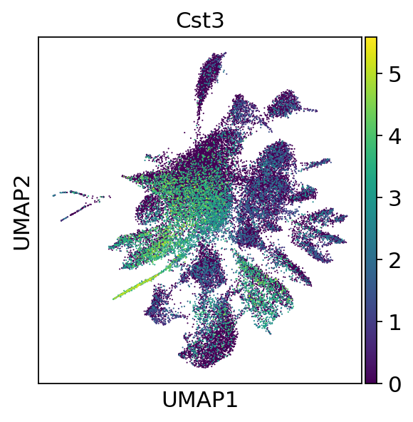

sc.pl.umap(adata, color=["Cst3"], use_raw=False)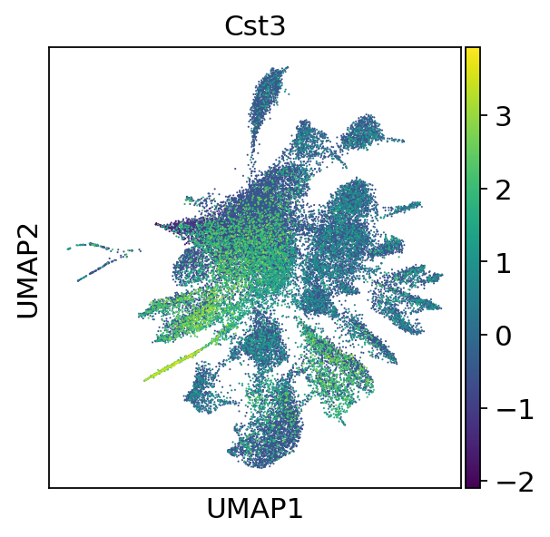

sc.pl.embedding(adata,"umap",color=["leiden"])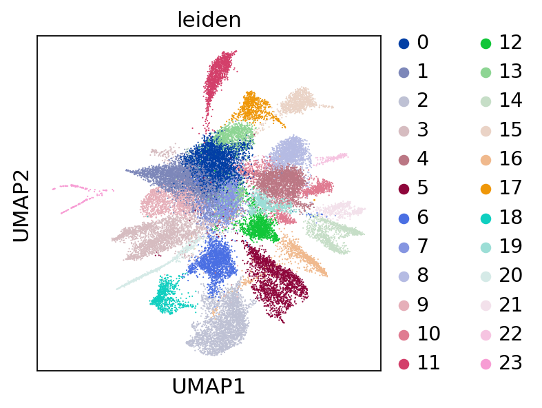

Add Spatial Coordinates

spatial_df = pd.read_csv("./Outs/WTH1092_filtered_feature_bc_matrix/cell_locations.tsv.gz",index_col=0,sep='\t')
spatial_df.columns = ['spatial_1', 'spatial_2']
spatial_df = pd.merge(adata.obs, spatial_df, left_index=True, right_index=True)[["spatial_1","spatial_2"]]
adata.obsm["spatial"] = spatial_df.values

adata

output

AnnData object with n_obs × n_vars = 32758 × 4960
obs: 'n_genes_by_counts', 'total_counts', 'total_counts_mt', 'pct_counts_mt', 'leiden'
var: 'gene_ids', 'feature_types', 'mt', 'n_cells_by_counts', 'mean_counts', 'pct_dropout_by_counts', 'total_counts', 'highly_variable', 'means', 'dispersions', 'dispersions_norm', 'mean', 'std'
uns: 'log1p', 'hvg', 'pca', 'neighbors', 'umap', 'tsne', 'leiden', 'leiden_colors'
obsm: 'X_pca', 'X_umap', 'X_tsne', 'spatial'
varm: 'PCs'
obsp: 'distances', 'connectivities'

sc.settings.set_figure_params(figsize=(10, 7))

Save the result.

sc.settings.set_figure_params(figsize=(15, 7))
sc.pl.embedding(adata,"spatial",color=["leiden"])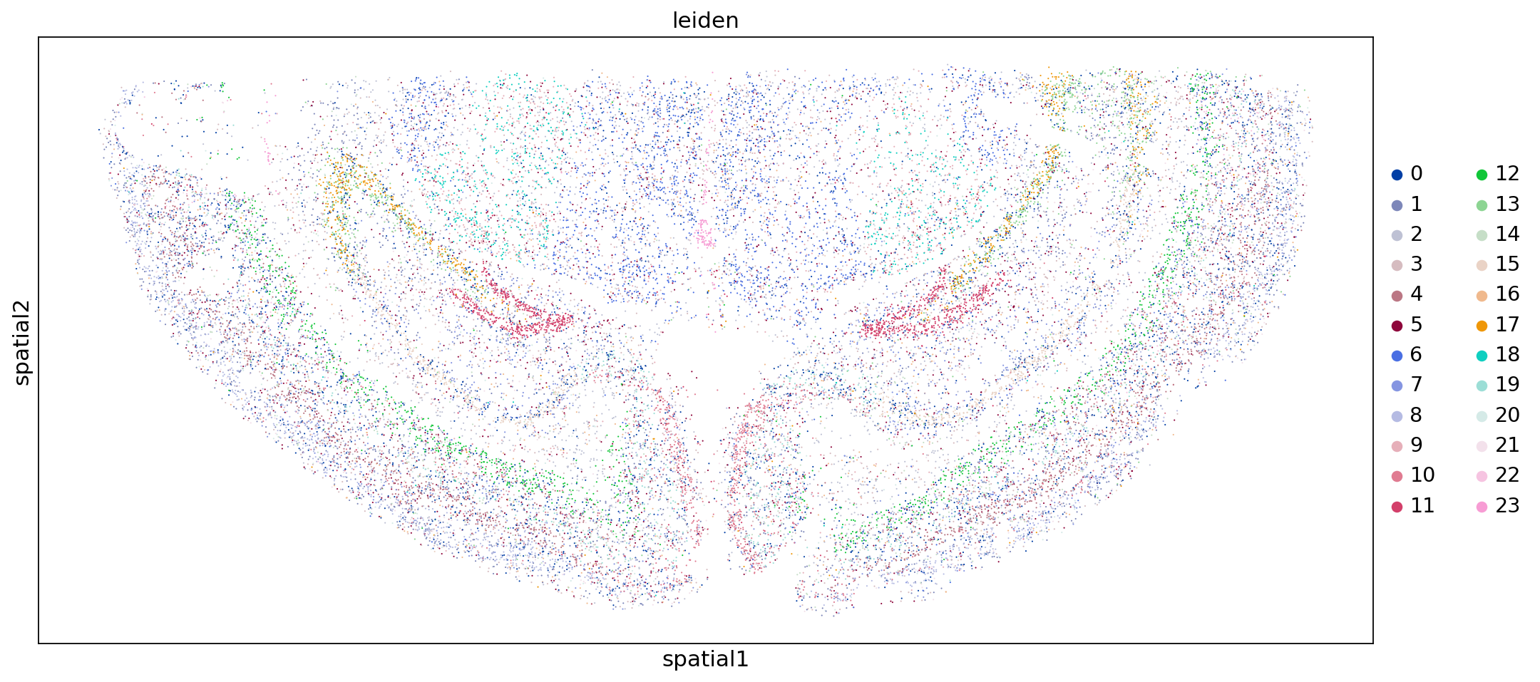

Add Cell Annotation Results

Next, we add the cell annotation results to each cell so we can see the distribution of different cell types in space.
The process of SeekSpace cell annotation is exactly the same as ordinary single-cell annotation.
We have previously annotated major groups and subgroups for the demo data, and the annotation results are in the annotation.csv file.
Next, we simply read and process it.

cell_anno = pd.read_csv("./annotation.csv",index_col=0,sep=',')

adata.obs = pd.merge(adata.obs,cell_anno,left_index=True,right_index=True)

adata

output

AnnData object with n_obs × n_vars = 32758 × 4960
obs: 'n_genes_by_counts', 'total_counts', 'total_counts_mt', 'pct_counts_mt', 'leiden', 'Sub_CellType', 'Main_CellType'
var: 'gene_ids', 'feature_types', 'mt', 'n_cells_by_counts', 'mean_counts', 'pct_dropout_by_counts', 'total_counts', 'highly_variable', 'means', 'dispersions', 'dispersions_norm', 'mean', 'std'
uns: 'log1p', 'hvg', 'pca', 'neighbors', 'umap', 'tsne', 'leiden', 'leiden_colors'
obsm: 'X_pca', 'X_umap', 'X_tsne', 'spatial'
varm: 'PCs'
obsp: 'distances', 'connectivities'

sc.settings.set_figure_params(figsize=(7, 7))
sc.pl.embedding(adata,"umap",color=["Main_CellType"])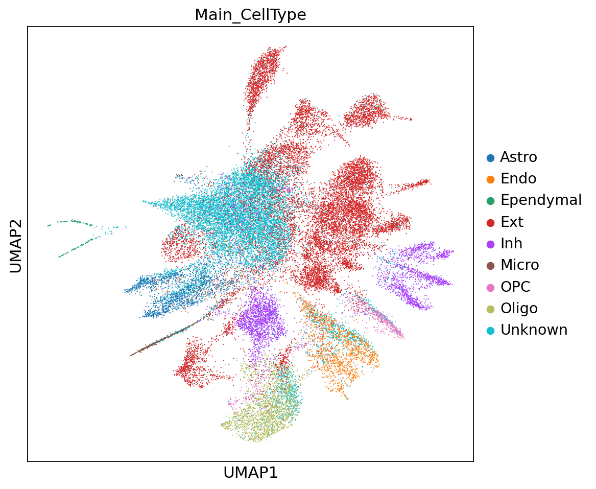

sc.settings.set_figure_params(figsize=(7, 7))
sc.pl.embedding(adata,"umap",color=[ "Sub_CellType"])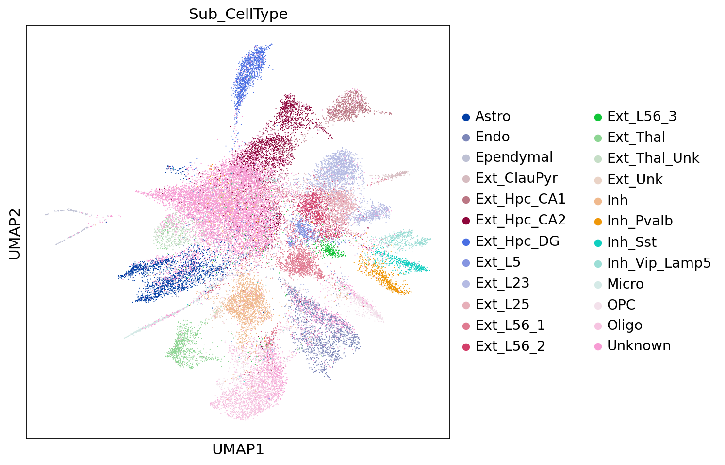

sc.settings.set_figure_params(figsize=(15, 7))
sc.pl.embedding(adata,"spatial",color=["Main_CellType"])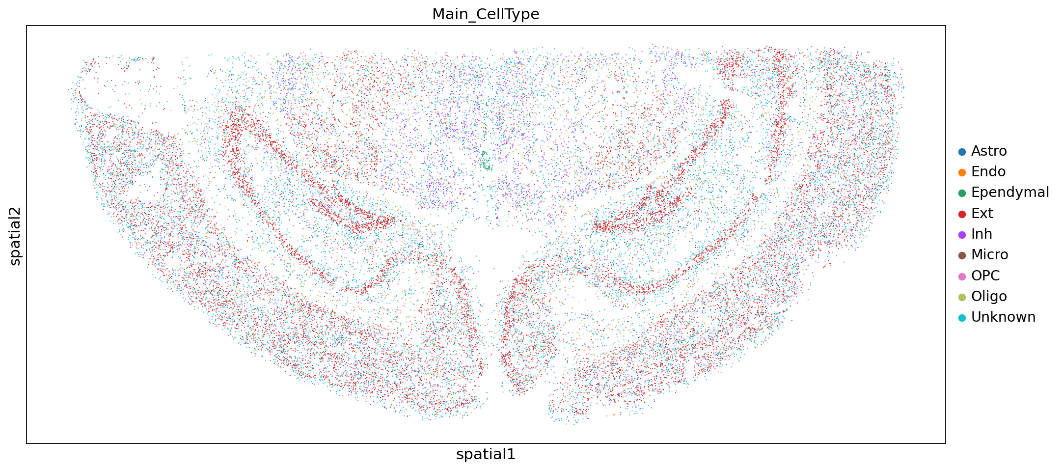

sc.settings.set_figure_params(figsize=(15, 7))
sc.pl.embedding(adata,"spatial",color=["Sub_CellType"])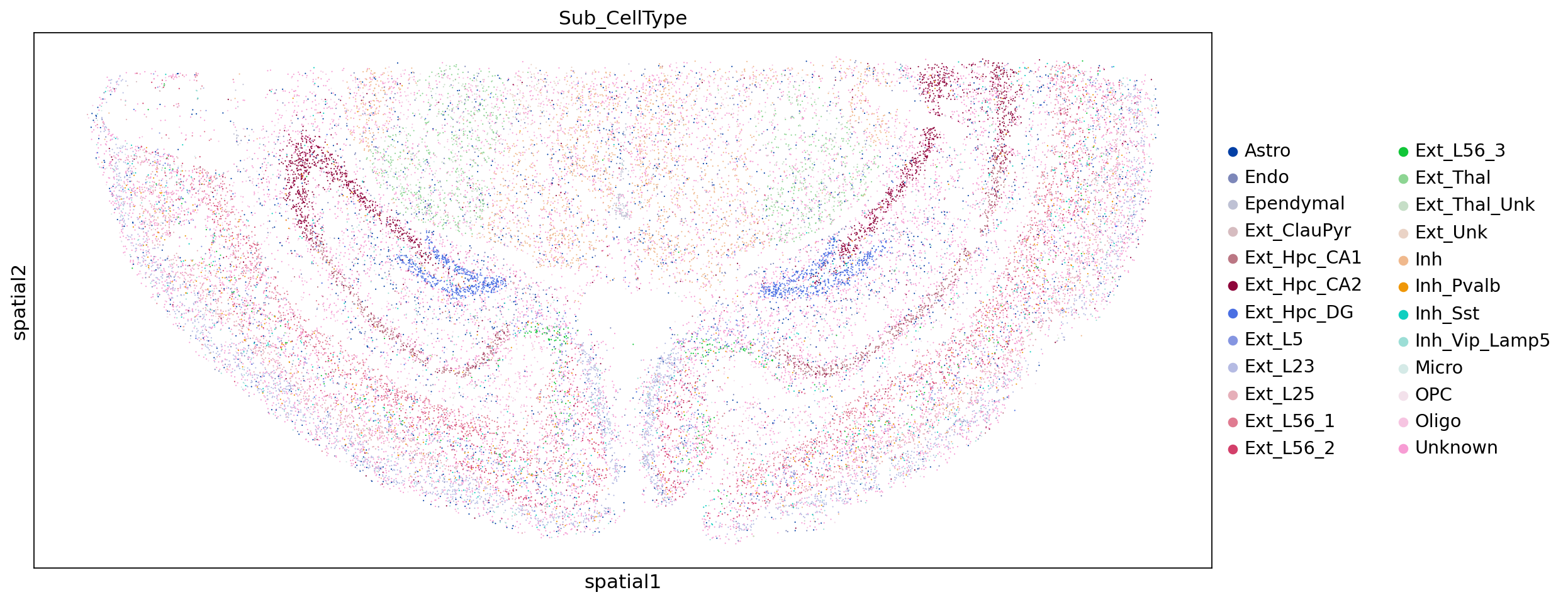

adata.write("WTH1092_demo_mouse_brain.h5ad")