SeekSpace 空间转录组数据分析教程 (Scanpy / 小鼠脑)

作者: SeekGene

时长: 9 分钟

字数: 1.8k 字

更新: 2026-02-28

阅读: 0 次

空间转录组 Notebooks 分析指南 基础分析

背景信息

本⽂档是关于寻因 SeekSpace 技术所得到的数据及其 scanpy 分析⽅法的说明。
寻因 SeekSpace 技术可以检测到单细胞精度的基因表达数据，同时也能定位出每个细胞在组织中的空间坐标。
SeekSpace 的数据分析简便易学，能够很方便地兼容常见单细胞转录组的分析软件，例如 Seurat 和 scanpy。
本数据为基于 SeekSpace 技术的⼩⿏脑的空间数据。数据中包含 32,758 个细胞的单细胞转录组矩阵，空间坐标矩阵，组织 DAPI 染⾊图⽚和 HE 图片。

⽂件说明

SeekSpace 技术的配套的基础数据处理的软件是 SeekSpace® Tools，该软件可以从测序文库中识别细胞的表达信息，同时可以识别出每个细胞在空间上的位置。
经过 SeekSpace® Tools 软件处理之后所得到的结果文件格式如下：

├── WTH1092_filtered_feature_bc_matrix # 表达矩阵⽬录，可以使⽤Seurat 的 Read10X 命令进⾏读取
│ ├── barcodes.tsv.gz
│ ├── features.tsv.gz
│ ├── matrix.mtx.gz
│ └── cell_locations.tsv.gz 为⼩⿏脑测序数据中细胞的空间坐标⽂件。第 1 列是 barcode，顺序与 matrix 中的 filtered_feature_bc_matrix/barcode 中细胞的顺序⼀致；第 2 列和第 3 列分别为该 barcode 所代表的细胞的空间位置（即空间芯⽚上的像素坐标）。

├── WTH1092_aligned_DAPI.png # 为⼩⿏脑组织切⽚的 DAPI 染⾊图⽚
├── WTH1092_aligned_HE.png
├── WTH1092_aligned_HE_TIMG.png
├── seekspace_of_Seurat.ipynb # 为使⽤Seurat 分析该⼩⿏脑空间数据的 jupyter 示例⽂件
└── seekspace_of_scanpy.ipynb # 为使⽤scanpy 分析该⼩⿏脑空间数据的 jupyter 示例⽂件
SeekSpace 技术中一个像素点的大小是约为 0.2653 微米，将像素点的坐标乘以 0.2653 即可转换计算细胞在真实空间上的距离。

import scanpy# Core scverse libraries
import scanpy as sc
import anndata as ad
import pandas as pd
# Data retrieval
import pooch

import warnings  
warnings.filterwarnings("ignore")

sc.settings.verbosity = 3  # verbosity: errors (0), warnings (1), info (2), hints (3)
sc.logging.print_header()
sc.settings.set_figure_params(dpi=80, facecolor="white")

output

scanpy==1.9.8 anndata==0.9.2 umap==0.5.6 numpy==1.22.4 scipy==1.10.1 pandas==2.0.3 scikit-learn==1.3.2 statsmodels==0.14.1 igraph==0.9.9 pynndescent==0.5.12

读取数据矩阵

adata = sc.read_10x_mtx(
    "./Outs/WTH1092_filtered_feature_bc_matrix/",
    cache=True
)

output

... reading from cache file cache/Outs-WTH1092_filtered_feature_bc_matrix-matrix.h5ad

adata.var_names_make_unique()

adata

output

AnnData object with n_obs × n_vars = 32758 × 32285
var: 'gene_ids', 'feature_types'

降维聚类

## Preprocessing
adata.var["mt"] = adata.var_names.str.startswith("mt-")
sc.pp.calculate_qc_metrics(
    adata, qc_vars=["mt"], percent_top=None, log1p=False, inplace=True
)

sc.pp.normalize_total(adata, target_sum=1e4)
sc.pp.log1p(adata)
sc.pp.highly_variable_genes(adata, min_mean=0.0125, max_mean=3, min_disp=0.5)

adata.raw = adata
adata = adata[:, adata.var.highly_variable]
sc.pp.regress_out(adata, ["total_counts", "pct_counts_mt"])
sc.pp.scale(adata, max_value=10)

output

normalizing counts per cell
finished (0:00:00)
extracting highly variable genes
finished (0:00:01)
--> added
'highly_variable', boolean vector (adata.var)
'means', float vector (adata.var)
'dispersions', float vector (adata.var)
'dispersions_norm', float vector (adata.var)
regressing out ['total_counts', 'pct_counts_mt']
sparse input is densified and may lead to high memory use
finished (0:02:49)

## Principal component analysis
sc.tl.pca(adata, svd_solver="arpack")

output

computing PCA
on highly variable genes
with n_comps=50
finished (0:00:15)

## Computing the neighborhood graph
sc.pp.neighbors(adata, n_neighbors=10, n_pcs=40)

output

computing neighbors
using 'X_pca' with n_pcs = 40
finished: added to \`.uns['neighbors']\`
\`.obsp['distances']\`, distances for each pair of neighbors
\`.obsp['connectivities']\`, weighted adjacency matrix (0:00:23)

## Embedding the neighborhood graph
#sc.tl.paga(adata)
#sc.pl.paga(adata, plot=False)  # remove `plot=False` if you want to see the coarse-grained graph
#sc.tl.umap(adata, init_pos='paga')

sc.tl.umap(adata)
sc.tl.tsne(adata)

output

computing UMAP
finished: added
'X_umap', UMAP coordinates (adata.obsm) (0:00:21)
computing tSNE
using 'X_pca' with n_pcs = 50
using sklearn.manifold.TSNE
finished: added
'X_tsne', tSNE coordinates (adata.obsm) (0:01:44)

## Clustering the neighborhood graph
sc.tl.leiden(
    adata,
    resolution=0.9,
    random_state=0,
    n_iterations=2,
    directed=False,
)

output

running Leiden clustering
finished: found 24 clusters and added
'leiden', the cluster labels (adata.obs, categorical) (0:00:01)

sc.pl.umap(adata, color=['Cst3'])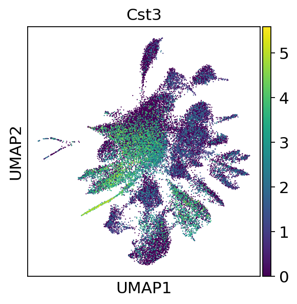

sc.pl.umap(adata, color=["Cst3"], use_raw=False)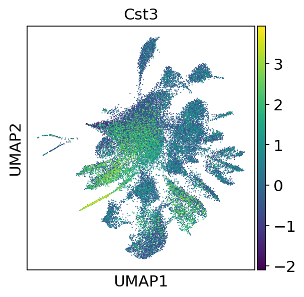

sc.pl.embedding(adata,"umap",color=["leiden"])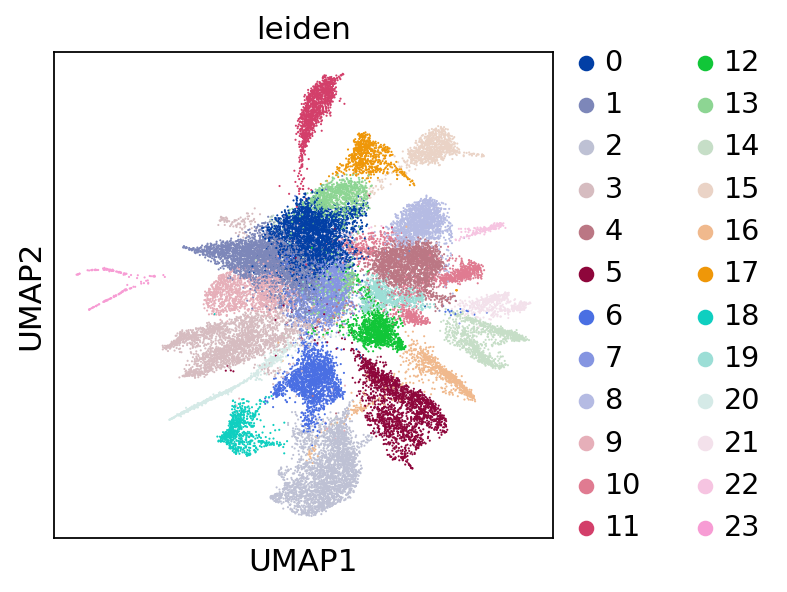

添加空间坐标

spatial_df = pd.read_csv("./Outs/WTH1092_filtered_feature_bc_matrix/cell_locations.tsv.gz",index_col=0,sep='\t')
spatial_df.columns = ['spatial_1', 'spatial_2']
spatial_df = pd.merge(adata.obs, spatial_df, left_index=True, right_index=True)[["spatial_1","spatial_2"]]
adata.obsm["spatial"] = spatial_df.values

adata

output

AnnData object with n_obs × n_vars = 32758 × 4960
obs: 'n_genes_by_counts', 'total_counts', 'total_counts_mt', 'pct_counts_mt', 'leiden'
var: 'gene_ids', 'feature_types', 'mt', 'n_cells_by_counts', 'mean_counts', 'pct_dropout_by_counts', 'total_counts', 'highly_variable', 'means', 'dispersions', 'dispersions_norm', 'mean', 'std'
uns: 'log1p', 'hvg', 'pca', 'neighbors', 'umap', 'tsne', 'leiden', 'leiden_colors'
obsm: 'X_pca', 'X_umap', 'X_tsne', 'spatial'
varm: 'PCs'
obsp: 'distances', 'connectivities'

sc.settings.set_figure_params(figsize=(10, 7))

Save the result.

sc.settings.set_figure_params(figsize=(15, 7))
sc.pl.embedding(adata,"spatial",color=["leiden"])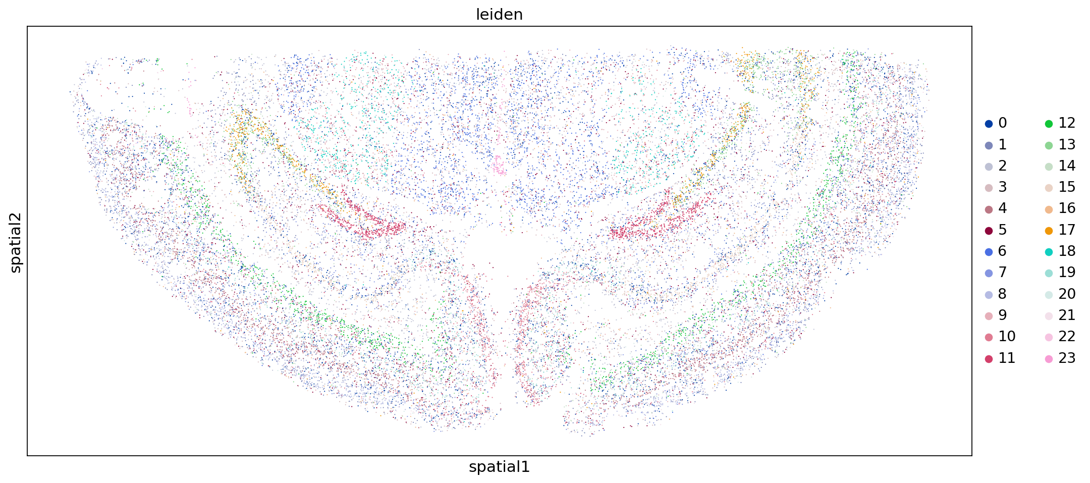

添加细胞注释结果

接下来我们再把细胞的注释结果添加到每个细胞上，这样我们就可以看不同的细胞类型在空间上的分布情况了。
SeekSpace 细胞注释的过程，跟普通的单细胞注释的过程完全一致。
我们之前已经对 demo 数据进行了大群和亚群的注释，注释的结果文件放在了 anntation.csv 文件中。
接下来我们简单的读入处理一下。

cell_anno = pd.read_csv("./annotation.csv",index_col=0,sep=',')

adata.obs = pd.merge(adata.obs,cell_anno,left_index=True,right_index=True)

adata

output

AnnData object with n_obs × n_vars = 32758 × 4960
obs: 'n_genes_by_counts', 'total_counts', 'total_counts_mt', 'pct_counts_mt', 'leiden', 'Sub_CellType', 'Main_CellType'
var: 'gene_ids', 'feature_types', 'mt', 'n_cells_by_counts', 'mean_counts', 'pct_dropout_by_counts', 'total_counts', 'highly_variable', 'means', 'dispersions', 'dispersions_norm', 'mean', 'std'
uns: 'log1p', 'hvg', 'pca', 'neighbors', 'umap', 'tsne', 'leiden', 'leiden_colors'
obsm: 'X_pca', 'X_umap', 'X_tsne', 'spatial'
varm: 'PCs'
obsp: 'distances', 'connectivities'

sc.settings.set_figure_params(figsize=(7, 7))
sc.pl.embedding(adata,"umap",color=["Main_CellType"])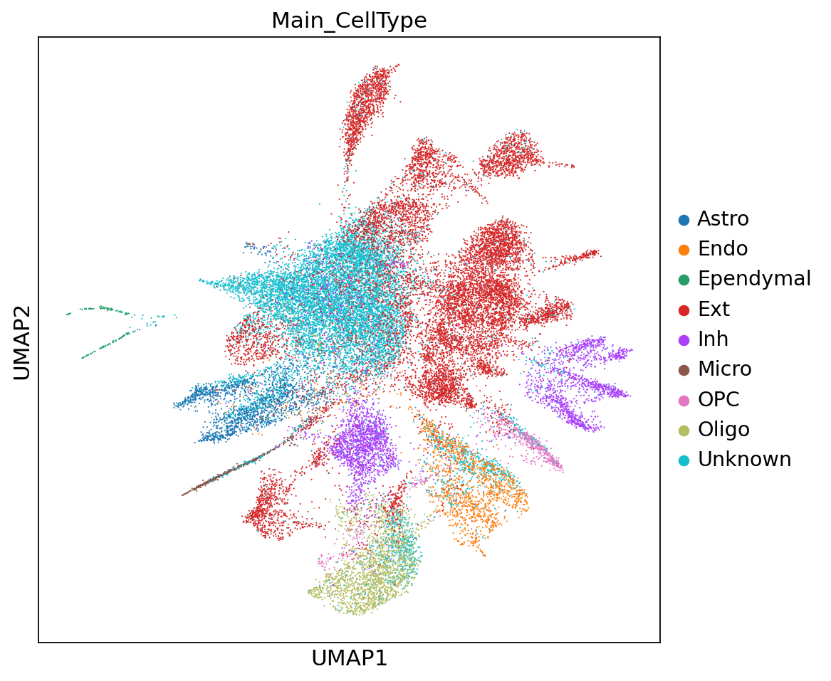

sc.settings.set_figure_params(figsize=(7, 7))
sc.pl.embedding(adata,"umap",color=[ "Sub_CellType"])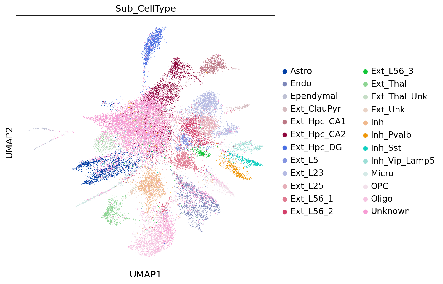

sc.settings.set_figure_params(figsize=(15, 7))
sc.pl.embedding(adata,"spatial",color=["Main_CellType"])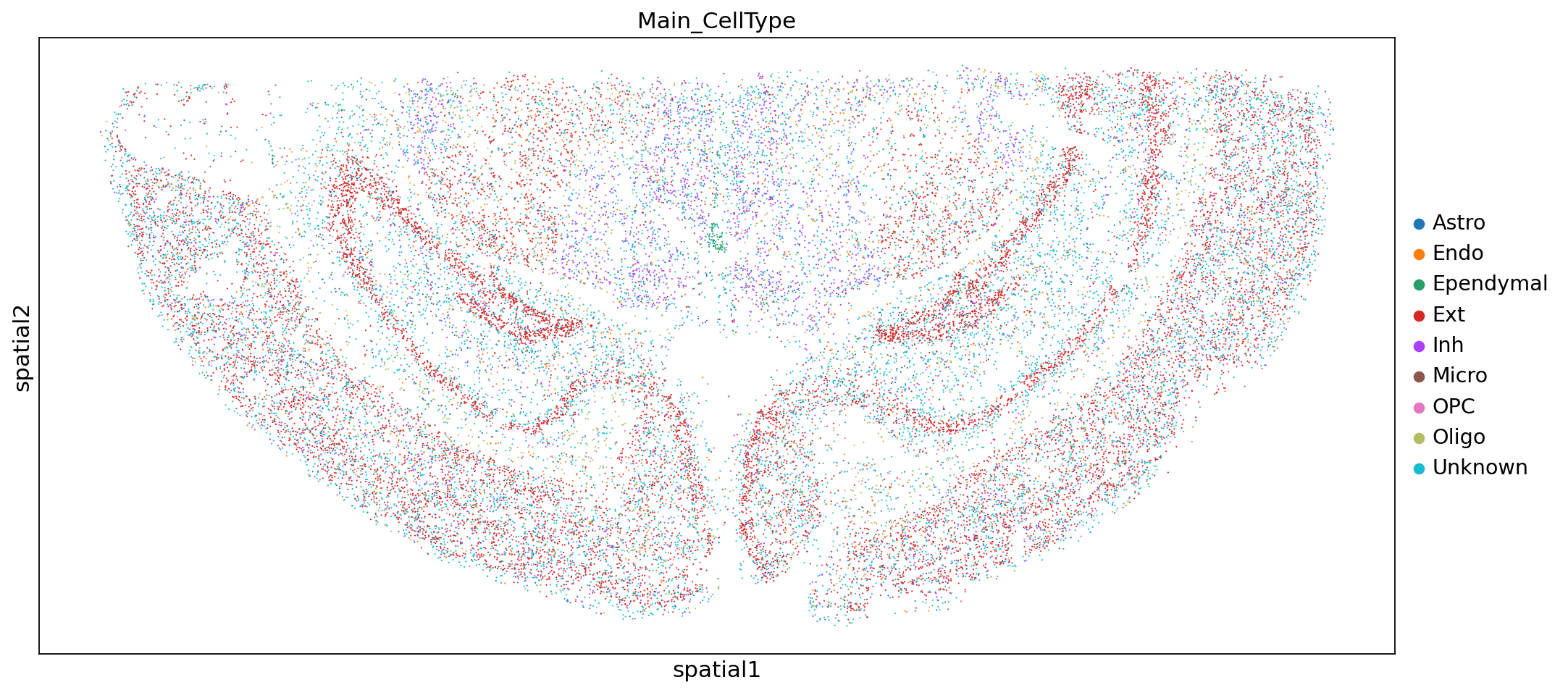

sc.settings.set_figure_params(figsize=(15, 7))
sc.pl.embedding(adata,"spatial",color=["Sub_CellType"])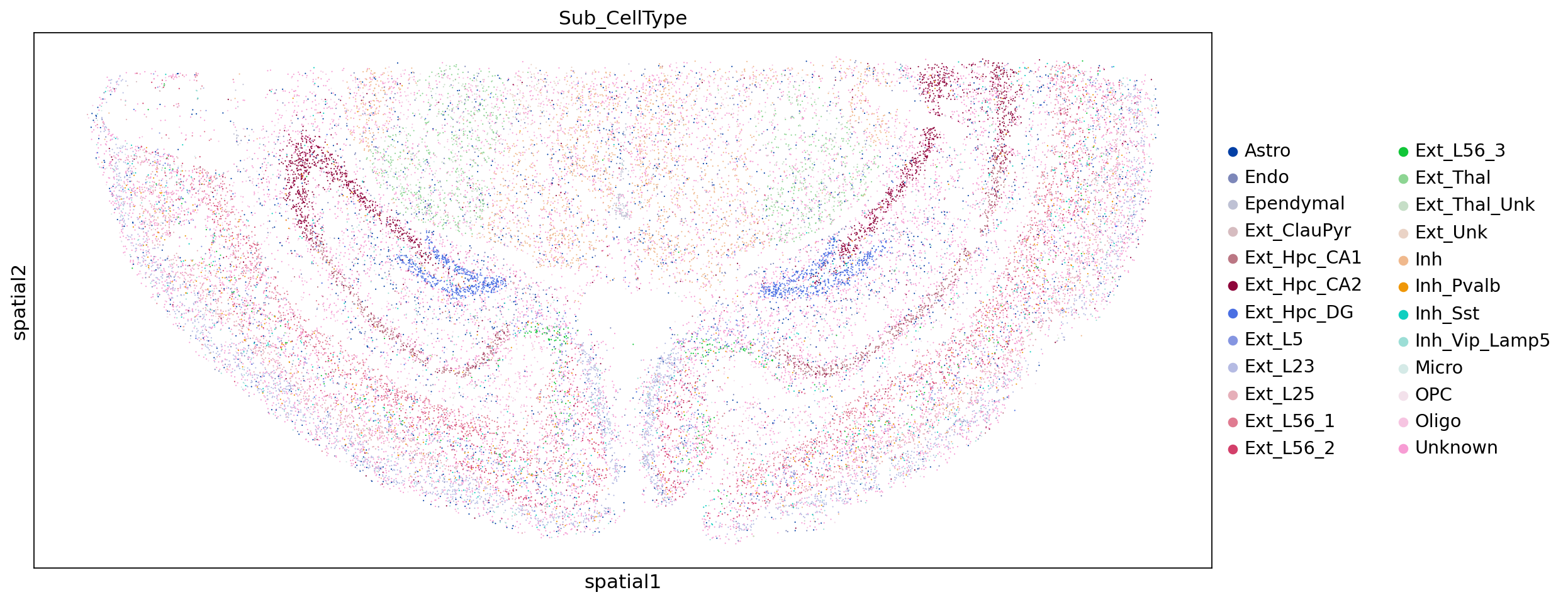

adata.write("WTH1092_demo_mouse_brain.h5ad")