SeekSpace Advanced Analysis: Spatial Cell Type Density Plotting
Time: 8 min
Words: 1.4k words
Updated: 2026-02-28
Reads: 0 times
python
import numpy as np
import pandas as pd
import matplotlib.pyplot as plt
from scipy.stats import gaussian_kde
from mpl_toolkits.mplot3d import Axes3D
Data Loading
First use R to save spatial coordinates and annotation results from rds
Read Spatial Coordinates
python
spatial_df = pd.read_csv("/PROJ2/FLOAT/weichendan/seekspace/SGS2401017/allsamples/00data/down_oss/ndGBM_5_2/ndGBM_5_2_barcode_centers.csv",index_col=0,sep=',')
spatial_df.drop(columns=['RNA_snn_res.0.8'], inplace=True)
Read Annotation Results
python
#celltype_df = pd.read_csv('/PROJ2/FLOAT/weichendan/seekspace/SGS2401017/allsamples/08mistyR/ndGBM_5_2_celltype.csv', index_col=0)
celltype_df = pd.read_csv("/PROJ2/FLOAT/weichendan/seekspace/SGS2401017/updata_allsamples/00data/scanpy_obs.csv")
celltype_df = celltype_df.drop(celltype_df.columns[0], axis=1)
#celltype_df['new_cell_id'] = celltype_df['new_cell_id'].str.replace('_9', '')
celltype_df['new_cell_id'] = celltype_df['new_cell_id'].str.replace(r'_\d+$', '', regex=True)
celltype_df = celltype_df.set_index('new_cell_id')
celltype_df = celltype_df[celltype_df['sample_id'].str.contains("ndGBM_5_2")]
python
spatial_df = spatial_df[spatial_df.index.isin(celltype_df.index)]
spatial_df = spatial_df.reindex(celltype_df.index)
Merge Data
python
merged_df = pd.merge(celltype_df, spatial_df, left_index=True, right_index=True,how="inner")python
merged_df| sample_id | cell_type | all_celltype | new_group | x | y | |
|---|---|---|---|---|---|---|
| new_cell_id | ||||||
| AGAGCCCCGATAGCTACCCTAATAACG | ndGBM_5_2 | Glioma | AC | GBM | 27913 | 15055 |
| CACCGTTATGGGAAACGTCCTATTAGG | ndGBM_5_2 | Fibroblast | Fibroblast | GBM | 29920 | 4106 |
| GCCATTCTACGCCTTTGCTAAGTACGA | ndGBM_5_2 | Glioma | AC | GBM | 34538 | 1969 |
| TAAGTCGCGACATCCGGCTAAGTACGA | ndGBM_5_2 | Oligodendrocyte | Oligodendrocyte | GBM | 27680 | 10535 |
| TACGTCCTACGAAGTGGGGACTGTGGA | ndGBM_5_2 | Fibroblast | Fibroblast | GBM | 43135 | 11168 |
| ... | ... | ... | ... | ... | ... | ... |
| CGCGTGACGATGCAAGGAAGGCACTAT | ndGBM_5_2 | Endothelial_cell | Endothelial_cell | GBM | 33528 | 12544 |
| GCCAGGTATGAGTCCGGGGACTGTGGA | ndGBM_5_2 | Endothelial_cell | Endothelial_cell | GBM | 40550 | 7503 |
| TGGGTTAATGACGTCGAAAGGCACTAT | ndGBM_5_2 | Endothelial_cell | Endothelial_cell | GBM | 20952 | 13660 |
| CCCGGAACGAGTCAGCCCCTAATAACG | ndGBM_5_2 | Endothelial_cell | Endothelial_cell | GBM | 41631 | 16713 |
| TCAGGGCGCTTTCTATCAGCGACGGAT | ndGBM_5_2 | Endothelial_cell | Endothelial_cell | GBM | 34379 | 11688 |
14055 rows × 6 columns
Plot 3D Spatial Density Map
Taking cell type AC as an example, plot its 3D spatial density map
python
merged_df1 = merged_df[merged_df['all_celltype']=="AC"][['x', 'y']]

# Calculate Density Distribution
xy = np.vstack([merged_df1.x, merged_df1.y])
kde = gaussian_kde(xy, bw_method=0.2)
xmin, xmax = merged_df1.x.min(), merged_df1.x.max()
ymin, ymax = merged_df1.y.min(), merged_df1.y.max()
xgrid = np.linspace(xmin, xmax, 200)
ygrid = np.linspace(ymin, ymax, 200)
X, Y = np.meshgrid(xgrid, ygrid)
Z = kde(np.vstack([X.ravel(), Y.ravel()])).reshape(X.shape)

# Create Canvas
fig = plt.figure(figsize=(15, 5))

# ---------------------------
# 3D Density Plot (Key View Settings)
# ---------------------------
ax3d = fig.add_subplot(111, projection='3d')

### Set Length:Width:Height
ax3d.set_box_aspect([15, 5, 5])

## Remove Grid
ax3d.grid(False)

# Plot Density Surface
surf = ax3d.plot_surface(X, Y, Z, cmap='RdYlGn_r',
                        rstride=5, cstride=5,
                        alpha=1, antialiased=True,
                        edgecolor='none')

# View Angle Parameters (Key Adjustment)
ax3d.view_init(elev=25, azim=-90)  # Adjust axis projection direction via azim
#ax3d.set_proj_type('ortho')         # Orthographic projection to eliminate perspective distortion

# Sync Axis Ranges
ax3d.set_xlim(xmin, xmax)
ax3d.set_ylim(ymin, ymax)
ax3d.set_zlim(0, Z.max()*1.1)

# Remove Axis Ticks
ax3d.set_xticks([])
ax3d.set_yticks([])
ax3d.set_zticks([])

# Remove Axis Lines
ax3d.xaxis.line.set_color((0,0,0,0))
ax3d.yaxis.line.set_color((0,0,0,0))
ax3d.zaxis.line.set_color((0,0,0,0))

# Remove Axis Labels
ax3d.set_xlabel('')
ax3d.set_ylabel('')
ax3d.set_zlabel('')

# Hide Redundant Labels
ax3d.set_xticklabels([])
ax3d.set_yticklabels([])
#ax3d.set_zlabel('Density', labelpad=15, fontsize=12)
# Make background and three walls white
ax3d.set_facecolor('white')
ax3d.xaxis.set_pane_color((1.0, 1.0, 1.0, 1.0))
ax3d.yaxis.set_pane_color((1.0, 1.0, 1.0, 1.0))
ax3d.zaxis.set_pane_color((1.0, 1.0, 1.0, 1.0))

plt.subplots_adjust(left=0, right=1, top=1, bottom=0)

#plt.savefig('output.png', dpi=300)
plt.show()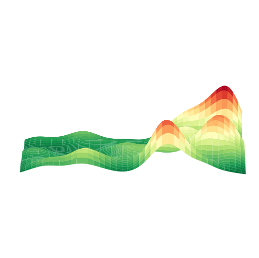
Plot 3D Spatial Density Mapping
Taking cell type AC as an example, plot its 3D spatial density mapping
python
merged_df1 = merged_df[merged_df['all_celltype']=="AC"][['x', 'y']]

# Calculate Density Distribution
xy = np.vstack([merged_df1.x, merged_df1.y])
kde = gaussian_kde(xy, bw_method=0.2)
xmin, xmax = merged_df1.x.min(), merged_df1.x.max()
ymin, ymax = merged_df1.y.min(), merged_df1.y.max()
xgrid = np.linspace(xmin, xmax, 200)
ygrid = np.linspace(ymin, ymax, 200)
X, Y = np.meshgrid(xgrid, ygrid)
Z = kde(np.vstack([X.ravel(), Y.ravel()])).reshape(X.shape)

# Create Canvas
fig = plt.figure(figsize=(15, 5))

# ---------------------------
# 3D Density Plot (Key View Settings)
# ---------------------------
ax3d = fig.add_subplot(111, projection='3d')

### Set Length:Width:Height
ax3d.set_box_aspect([15, 5, 0.1])

## Remove Grid
ax3d.grid(False)

# Plot Density Surface
surf = ax3d.plot_surface(X, Y, Z, cmap='RdYlGn_r',
                        rstride=5, cstride=5,
                        alpha=1, antialiased=True,
                        edgecolor='none')

# View Angle Parameters (Key Adjustment)
ax3d.view_init(elev=25, azim=-90)  # Adjust axis projection direction via azim
#ax3d.set_proj_type('ortho')         # Orthographic projection to eliminate perspective distortion

# Sync Axis Ranges
ax3d.set_xlim(xmin, xmax)
ax3d.set_ylim(ymin, ymax)
ax3d.set_zlim(0, Z.max()*1.1)

# Remove Axis Ticks
ax3d.set_xticks([])
ax3d.set_yticks([])
ax3d.set_zticks([])

# Remove Axis Lines
ax3d.xaxis.line.set_color((0,0,0,0))
ax3d.yaxis.line.set_color((0,0,0,0))
ax3d.zaxis.line.set_color((0,0,0,0))

# Remove Axis Labels
ax3d.set_xlabel('')
ax3d.set_ylabel('')
ax3d.set_zlabel('')

# Hide Redundant Labels
ax3d.set_xticklabels([])
ax3d.set_yticklabels([])
#ax3d.set_zlabel('Density', labelpad=15, fontsize=12)
# Make background and three walls white
ax3d.set_facecolor('white')
ax3d.xaxis.set_pane_color((1.0, 1.0, 1.0, 1.0))
ax3d.yaxis.set_pane_color((1.0, 1.0, 1.0, 1.0))
ax3d.zaxis.set_pane_color((1.0, 1.0, 1.0, 1.0))

plt.subplots_adjust(left=0, right=1, top=1, bottom=0)

#plt.savefig('output.png', dpi=300)
plt.show()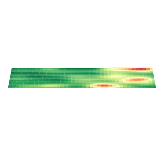
Plot 2D Density Map
python
fig2d, ax2d = plt.subplots(figsize=(6, 4))
contour = ax2d.contourf(X, Y, Z, levels=20, cmap='RdYlGn_r')

# Axis Settings
ax2d.set(xlim=(xmin, xmax), ylim=(ymin, ymax), aspect='equal')

# Remove Axis Ticks
ax2d.set_xticks([])
ax2d.set_yticks([])

# Remove Axis Labels
ax2d.set_xlabel('')
ax2d.set_ylabel('')

plt.show()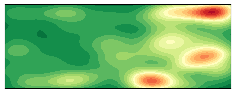
python
python