SeekSpace Advanced Analysis: Neighborhood Enrichment and Co-occurrence Analysis Based on Squidpy

Author: SeekGene

Time: 18 min

Words: 3.5k words

Updated: 2026-02-28

Reads: 0 times

Spatial-seq Analysis Guide Notebooks Niche Analysis

Select execution environment 'cellcharter-env'

Squidpy is a tool for analyzing and visualizing spatial data. Built on top of scanpy and anndata, it inherits modularity and scalability. It provides analysis tools utilizing spatial coordinates of data and tissue images (if available).
Analysis content mainly includes:

• Neighborhood Enrichment
• Co-occurrence Analysis
• Variable Genes
• Dispersion Level

Data Loading and Preprocessing

Read based on three matrix files, additionally adding spatial location and cell annotation (can be any cell clustering) results.

adata = sc.read_10x_mtx(
    "/PROJ2/FLOAT/weichendan/seekspace/WTH1092/demo_WTH1092/Outs/WTH1092_filtered_feature_bc_matrix/",
    cache=True
)

adata

output

AnnData object with n_obs × n_vars = 32758 × 32285
var: 'gene_ids', 'feature_types'

adata.var_names_make_unique() 
sc.pp.filter_cells(adata, min_genes=200)
sc.pp.filter_genes(adata, min_cells=3)

adata.var["mt"] = adata.var_names.str.startswith("mt-")
sc.pp.calculate_qc_metrics(
    adata, qc_vars=["mt"], percent_top=None, log1p=False, inplace=True
)

adata = adata[adata.obs.n_genes_by_counts < 2500, :]
adata = adata[adata.obs.pct_counts_mt < 5, :].copy()

sc.pp.normalize_total(adata, target_sum=1e4)
sc.pp.log1p(adata)
sc.pp.highly_variable_genes(adata, min_mean=0.0125, max_mean=3, min_disp=0.5)

adata.raw = adata

adata = adata[:, adata.var.highly_variable]
sc.pp.regress_out(adata, ["total_counts", "pct_counts_mt"])
sc.pp.scale(adata, max_value=10)

sc.tl.pca(adata, svd_solver="arpack")
sc.pp.neighbors(adata, n_neighbors=10, n_pcs=40)
sc.tl.umap(adata)
sc.tl.tsne(adata)

output

/PROJ2/FLOAT/weichendan/software/micromamba/envs/cellcharter-env/lib/python3.9/site-packages/anndata/_core/anndata.py:1209: ImplicitModificationWarning: Trying to modify attribute \`.var\` of view, initializing view as actual.
df[key] = c
/PROJ2/FLOAT/weichendan/software/micromamba/envs/cellcharter-env/lib/python3.9/site-packages/tqdm/auto.py:21: TqdmWarning: IProgress not found. Please update jupyter and ipywidgets. See https://ipywidgets.readthedocs.io/en/stable/user_install.html
from .autonotebook import tqdm as notebook_tqdm

adata

output

AnnData object with n_obs × n_vars = 22512 × 3546
obs: 'n_genes', 'n_genes_by_counts', 'total_counts', 'total_counts_mt', 'pct_counts_mt'
var: 'gene_ids', 'feature_types', 'n_cells', 'mt', 'n_cells_by_counts', 'mean_counts', 'pct_dropout_by_counts', 'total_counts', 'highly_variable', 'means', 'dispersions', 'dispersions_norm', 'mean', 'std'
uns: 'log1p', 'hvg', 'pca', 'neighbors', 'umap', 'tsne'
obsm: 'X_pca', 'X_umap', 'X_tsne'
varm: 'PCs'
obsp: 'distances', 'connectivities'

spatial_df = pd.read_csv("/PROJ2/FLOAT/weichendan/seekspace/WTH1092/demo_WTH1092/Outs/WTH1092_filtered_feature_bc_matrix/cell_locations.tsv.gz",index_col=0,sep='\t')
spatial_df.columns = ["spatial_1","spatial_2"]
spatial_df = pd.merge(adata.obs, spatial_df, left_index=True, right_index=True)[["spatial_1","spatial_2"]]

adata.obsm["spatial"] = spatial_df.values

spatial_df

	spatial_1	spatial_2
TTGTGTTATGCAAGAGGTAGTCATACG	33195	11954
TGCGACGATGACGATACCTAAGTACGA	25664	15747
ACCTGAACGAAGGGTCAGCTCTGCTTC	36614	13290
CACTGGGTACGGTCGACCCTAATAACG	35019	10923
AAGATAGCGAAGGAGGGCTAAGTACGA	42849	13006
...	...	...
TCAAGCAGCTGTTACCATTCTGCGCTC	17118	14572
ACCCTTGCGAACTCAACGCTCTGCTTC	34011	13369
GTTCTATATGCGGACTGGCTCTGCTTC	15772	12816
TACCGAATACCTCCGACGCTCTGCTTC	21987	16150
AATGAAGGCTCTTGAACAGCGACGGAT	29200	4941

22512 rows × 2 columns

cell_anno = pd.read_csv("/PROJ2/FLOAT/weichendan/seekspace/WTH1092/annotation.csv",index_col=0)
cell_anno = cell_anno[["Main_CellType","Sub_CellType"]]

adata.obs = pd.merge(adata.obs,cell_anno,left_index=True,right_index=True)

adata

output

AnnData object with n_obs × n_vars = 22512 × 3546
obs: 'n_genes', 'n_genes_by_counts', 'total_counts', 'total_counts_mt', 'pct_counts_mt', 'Main_CellType', 'Sub_CellType'
var: 'gene_ids', 'feature_types', 'n_cells', 'mt', 'n_cells_by_counts', 'mean_counts', 'pct_dropout_by_counts', 'total_counts', 'highly_variable', 'means', 'dispersions', 'dispersions_norm', 'mean', 'std'
uns: 'log1p', 'hvg', 'pca', 'neighbors', 'umap', 'tsne'
obsm: 'X_pca', 'X_umap', 'X_tsne', 'spatial'
varm: 'PCs'
obsp: 'distances', 'connectivities'

Major Group Annotation Results:

sc.settings.set_figure_params(figsize=(10, 5))
sc.pl.embedding(adata,"spatial",color=["Main_CellType"])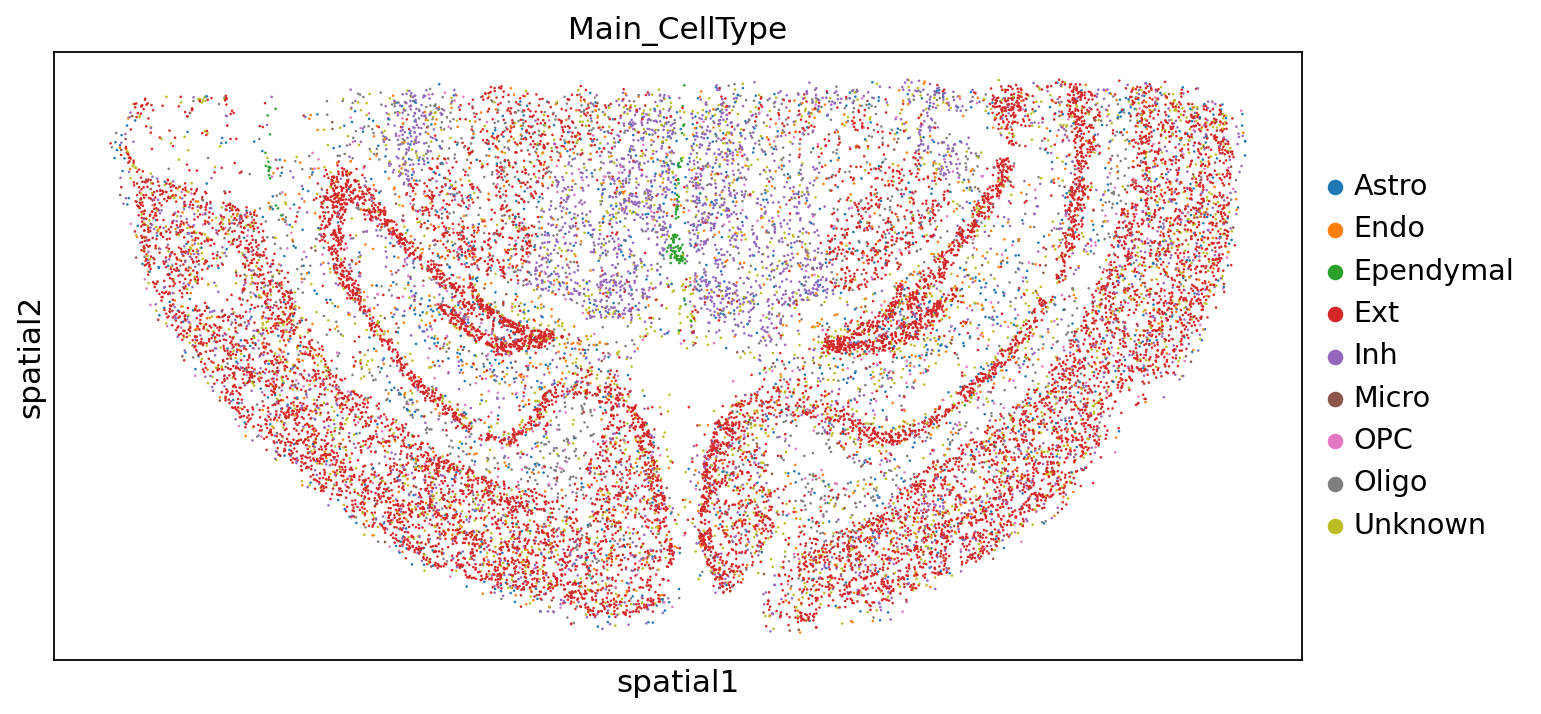

Subgroup Annotation Results:

sc.settings.set_figure_params(figsize=(10, 5))
sc.pl.embedding(adata,"spatial",color=["Sub_CellType"])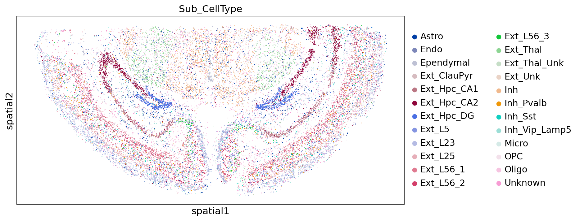

Neighborhood Enrichment

Calculating neighborhood enrichment helps us identify cell clusters sharing common neighborhood structures across the tissue.
In short, this is an enrichment score for cluster spatial proximity: if cells belonging to two different clusters are usually close to each other, they will have a high score and can be defined as enriched. On the other hand, if they are far apart and rarely neighbors, the score will be low and can be defined as depleted.

sq.gr.spatial_neighbors(adata)
sq.gr.nhood_enrichment(adata, cluster_key="Sub_CellType")

output

00%|██████████| 1000/1000 [00:01<00:00, 534.15/s]

adata

output

AnnData object with n_obs × n_vars = 22512 × 3546
obs: 'n_genes', 'n_genes_by_counts', 'total_counts', 'total_counts_mt', 'pct_counts_mt', 'Main_CellType', 'Sub_CellType'
var: 'gene_ids', 'feature_types', 'n_cells', 'mt', 'n_cells_by_counts', 'mean_counts', 'pct_dropout_by_counts', 'total_counts', 'highly_variable', 'means', 'dispersions', 'dispersions_norm', 'mean', 'std'
uns: 'log1p', 'hvg', 'pca', 'neighbors', 'umap', 'tsne', 'Main_CellType_colors', 'Sub_CellType_colors', 'spatial_neighbors', 'Sub_CellType_nhood_enrichment'
obsm: 'X_pca', 'X_umap', 'X_tsne', 'spatial'
varm: 'PCs'
obsp: 'distances', 'connectivities', 'spatial_connectivities', 'spatial_distances'

sq.pl.nhood_enrichment(adata, cluster_key="Sub_CellType", figsize=(5, 10))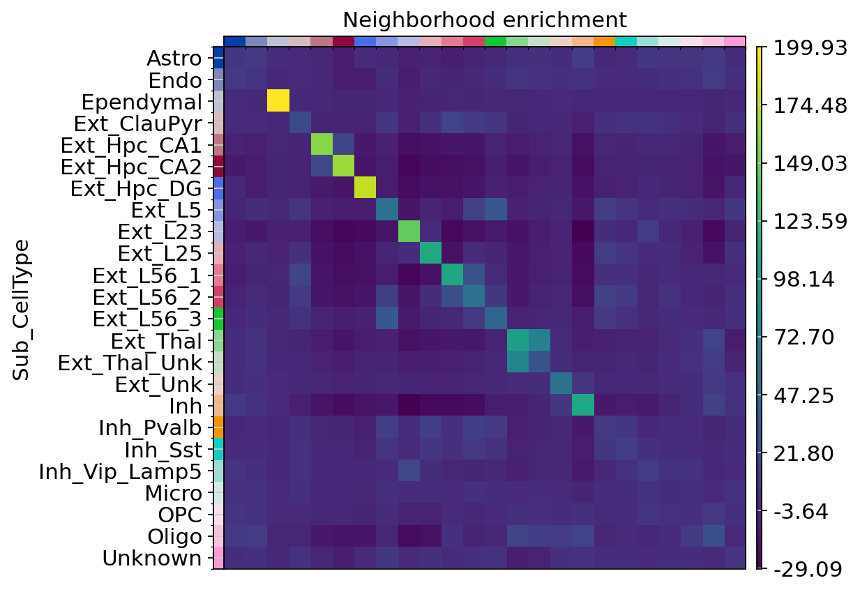

Figure Legend: Neighborhood enrichment analysis between cell clusters in spatial coordinates.

Spatial Dimension Co-occurrence Analysis

Besides neighborhood enrichment scores, we can visualize cluster co-occurrence in the spatial dimension. This is similar to the analysis above but runs on raw spatial coordinates rather than the data matrix.

sq.gr.co_occurrence(adata, cluster_key="Sub_CellType")

output

00%|██████████| 1/1 [03:23<00:00, 203.97s/]

adata

output

AnnData object with n_obs × n_vars = 22512 × 3546
obs: 'n_genes', 'n_genes_by_counts', 'total_counts', 'total_counts_mt', 'pct_counts_mt', 'Main_CellType', 'Sub_CellType'
var: 'gene_ids', 'feature_types', 'n_cells', 'mt', 'n_cells_by_counts', 'mean_counts', 'pct_dropout_by_counts', 'total_counts', 'highly_variable', 'means', 'dispersions', 'dispersions_norm', 'mean', 'std'
uns: 'log1p', 'hvg', 'pca', 'neighbors', 'umap', 'tsne', 'Main_CellType_colors', 'Sub_CellType_colors', 'spatial_neighbors', 'Sub_CellType_nhood_enrichment', 'Sub_CellType_co_occurrence'
obsm: 'X_pca', 'X_umap', 'X_tsne', 'spatial'
varm: 'PCs'
obsp: 'distances', 'connectivities', 'spatial_connectivities', 'spatial_distances'

np.unique(adata.obs['Sub_CellType'])

output

array(['Astro', 'Endo', 'Ependymal', 'Ext_ClauPyr', 'Ext_Hpc_CA1',
'Ext_Hpc_CA2', 'Ext_Hpc_DG', 'Ext_L23', 'Ext_L25', 'Ext_L5',
'Ext_L56_1', 'Ext_L56_2', 'Ext_L56_3', 'Ext_Thal', 'Ext_Thal_Unk',
'Ext_Unk', 'Inh', 'Inh_Pvalb', 'Inh_Sst', 'Inh_Vip_Lamp5', 'Micro',
'OPC', 'Oligo', 'Unknown'], dtype=object)

import matplotlib.pyplot as plt
sq.pl.co_occurrence(
    adata,
    cluster_key="Sub_CellType",
    clusters="Astro",
    figsize=(10, 4)
)
# Get legend on current axes (if any)
legend = plt.gca().get_legend()

if legend is not None:
    # Get legend handles and labels
    handles, labels = legend.legend_handles, [t.get_text() for t in legend.texts]   
    # Remove old legend
    legend.remove()
    # Add new legend and set ncol=2
    plt.legend(
        handles=handles,
        labels=labels,
        loc='center left',  # Or specify position, e.g., 'upper right'
        bbox_to_anchor=(1, 0.5), # Place to the right of axes (1 means outside right boundary)
        ncol=2,       # Set to two columns
    )

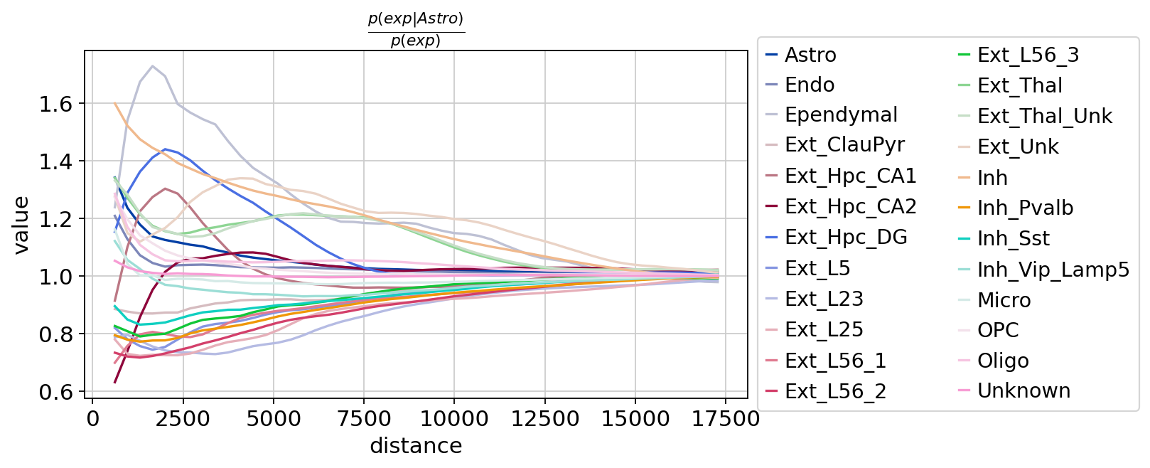
Figure Legend: Cluster co-occurrence score for each cell. In the tissue, as the distance threshold increases, the cluster co-occurrence score for each cell changes gradually. X-axis is distance, Y-axis is co-occurrence score.

Spatially Variable Genes Moran's I

Spatially Variable Genes (SVGs) refer to genes with significant variation in expression patterns across different spatial locations (e.g., different regions in tissue sections, different domains in developmental processes) in spatial transcriptomics data. These genes are usually closely related to tissue microenvironment, cell type distribution, developmental gradients, pathological states, etc., and are key entry points for resolving spatial tissue structure and functional heterogeneity. Next, we can find genes showing spatial patterns. Here, we provide a simple method based on the famous Moran's I statistic.

genes = adata[:, adata.var.highly_variable].var_names.values[:1000]
sq.gr.spatial_autocorr(
    adata,
    mode="moran",
    genes=genes,
    n_perms=100,
    n_jobs=1,
)

output

00%|██████████| 100/100 [00:51<00:00, 1.94/s]

adata

output

AnnData object with n_obs × n_vars = 22512 × 3546
obs: 'n_genes', 'n_genes_by_counts', 'total_counts', 'total_counts_mt', 'pct_counts_mt', 'Main_CellType', 'Sub_CellType'
var: 'gene_ids', 'feature_types', 'n_cells', 'mt', 'n_cells_by_counts', 'mean_counts', 'pct_dropout_by_counts', 'total_counts', 'highly_variable', 'means', 'dispersions', 'dispersions_norm', 'mean', 'std'
uns: 'log1p', 'hvg', 'pca', 'neighbors', 'umap', 'tsne', 'Main_CellType_colors', 'Sub_CellType_colors', 'spatial_neighbors', 'Sub_CellType_nhood_enrichment', 'Sub_CellType_co_occurrence', 'moranI'
obsm: 'X_pca', 'X_umap', 'X_tsne', 'spatial'
varm: 'PCs'
obsp: 'distances', 'connectivities', 'spatial_connectivities', 'spatial_distances'

Variable Gene Assessment Results:

adata.uns["moranI"].head(10)

	I	pval_norm	var_norm	pval_z_sim	pval_sim	var_sim	pval_norm_fdr_bh	pval_z_sim_fdr_bh	pval_sim_fdr_bh
Wfdc2	0.469195	0.0	0.000013	0.0	0.009901	0.000021	0.0	0.0	0.025987
Dpp10	0.339641	0.0	0.000013	0.0	0.009901	0.000017	0.0	0.0	0.025987
Tshz2	0.315615	0.0	0.000013	0.0	0.009901	0.000023	0.0	0.0	0.025987
Hpca	0.304144	0.0	0.000013	0.0	0.009901	0.000017	0.0	0.0	0.025987
Spag17	0.298851	0.0	0.000013	0.0	0.009901	0.000023	0.0	0.0	0.025987
Fibcd1	0.298201	0.0	0.000013	0.0	0.009901	0.000024	0.0	0.0	0.025987
Tmem212	0.261650	0.0	0.000013	0.0	0.009901	0.000011	0.0	0.0	0.025987
Ccdc146	0.261100	0.0	0.000013	0.0	0.009901	0.000021	0.0	0.0	0.025987
Synpo2	0.240745	0.0	0.000013	0.0	0.009901	0.000014	0.0	0.0	0.025987
Camk2n1	0.233325	0.0	0.000013	0.0	0.009901	0.000016	0.0	0.0	0.025987

Spatial expression of top 5 variable genes on tissue section:

adata.uns["moranI"].index[0:5]

output

Index(['Wfdc2', 'Dpp10', 'Tshz2', 'Hpca', 'Spag17'], dtype='object')

#sq.pl.spatial_scatter(adata, color=adata.uns["moranI"].index[0:5])
sc.pl.embedding(adata,"spatial",color=adata.uns["moranI"].index[0:4])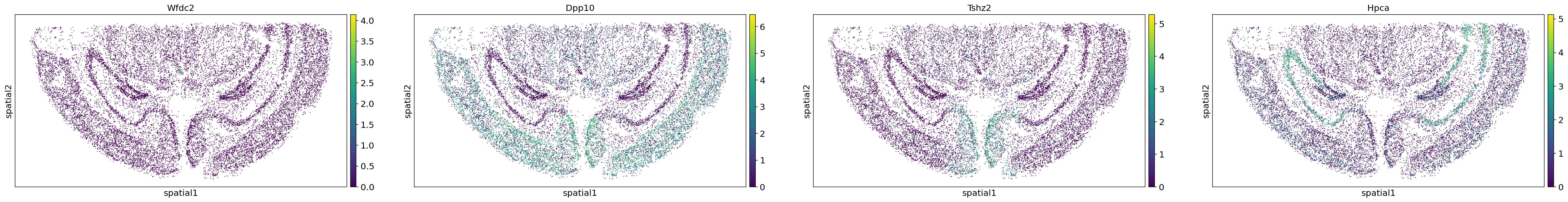

Figure Legend: Expression of four spatially variable genes (Wfdc2, Dpp10, Tshz2, and Hpca) calculated via Moran's I spatial autocorrelation analysis. These genes appear to exhibit distinct pattern characteristics and specific expression for different cell types.

Spatial Dispersion Level of Cell Clusters

Besides neighborhood enrichment scores, we can further investigate spatial organization of cell types in tissue using Ripley's statistics. Ripley's statistics allow analysts to assess whether discrete annotations (e.g., cell types) are aggregated, dispersed, or randomly distributed over the region of interest.

mode = "L"
sq.gr.ripley(adata, cluster_key="Sub_CellType", mode=mode, max_dist=500)

adata

output

AnnData object with n_obs × n_vars = 22512 × 3546
obs: 'n_genes', 'n_genes_by_counts', 'total_counts', 'total_counts_mt', 'pct_counts_mt', 'Main_CellType', 'Sub_CellType'
var: 'gene_ids', 'feature_types', 'n_cells', 'mt', 'n_cells_by_counts', 'mean_counts', 'pct_dropout_by_counts', 'total_counts', 'highly_variable', 'means', 'dispersions', 'dispersions_norm', 'mean', 'std'
uns: 'log1p', 'hvg', 'pca', 'neighbors', 'umap', 'tsne', 'Main_CellType_colors', 'Sub_CellType_colors', 'spatial_neighbors', 'Sub_CellType_nhood_enrichment', 'Sub_CellType_co_occurrence', 'moranI', 'Sub_CellType_ripley_L'
obsm: 'X_pca', 'X_umap', 'X_tsne', 'spatial'
varm: 'PCs'
obsp: 'distances', 'connectivities', 'spatial_connectivities', 'spatial_distances'

adata.uns["Sub_CellType_ripley_L"]

output

{'L_stat': bins Sub_CellType stats
0 0.000000 Astro 0.000000
1 10.204082 Astro 1.637580
2 20.408163 Astro 2.315888
3 30.612245 Astro 3.171160
4 40.816327 Astro 3.375957
... ... ... ...n 1195 459.183673 Unknown 60.034669
1196 469.387755 Unknown 61.332776
1197 479.591837 Unknown 62.609327
1198 489.795918 Unknown 63.813106
1199 500.000000 Unknown 64.839684

[1200 rows x 3 columns],
'sims_stat': bins simulations stats
0 0.000000 0 0.000000
1 10.204082 0 0.000000
2 20.408163 0 0.818790
3 30.612245 0 1.157944
4 40.816327 0 1.157944
... ... ... ...n 4995 459.183673 99 20.486117
4996 469.387755 99 20.713929
4997 479.591837 99 21.209662
4998 489.795918 99 21.694070
4999 500.000000 99 22.137633

[5000 rows x 3 columns],
'bins': array([ 0. , 10.20408163, 20.40816327, 30.6122449 ,
40.81632653, 51.02040816, 61.2244898 , 71.42857143,
81.63265306, 91.83673469, 102.04081633, 112.24489796,
122.44897959, 132.65306122, 142.85714286, 153.06122449,
163.26530612, 173.46938776, 183.67346939, 193.87755102,
204.08163265, 214.28571429, 224.48979592, 234.69387755,
244.89795918, 255.10204082, 265.30612245, 275.51020408,
285.71428571, 295.91836735, 306.12244898, 316.32653061,
326.53061224, 336.73469388, 346.93877551, 357.14285714,
367.34693878, 377.55102041, 387.75510204, 397.95918367,
408.16326531, 418.36734694, 428.57142857, 438.7755102 ,
448.97959184, 459.18367347, 469.3877551 , 479.59183673,
489.79591837, 500. ]),
'pvalues': array([[0. , 0.00990099, 0.00990099, ..., 0.00990099, 0.00990099,
0.00990099],
[0. , 0.00990099, 0.00990099, ..., 0.00990099, 0.00990099,
0.00990099],
[0. , 0. , 0.32673267, ..., 0.00990099, 0.00990099,
0.00990099],
...,
[0. , 0.06930693, 0.05940594, ..., 0. , 0. ,
0. ],
[0. , 0.00990099, 0.00990099, ..., 0.00990099, 0.00990099,
0.00990099],
[0. , 0.00990099, 0.00990099, ..., 0.00990099, 0.00990099,
0.00990099]])}

sq.pl.ripley(adata, cluster_key="Sub_CellType", mode=mode)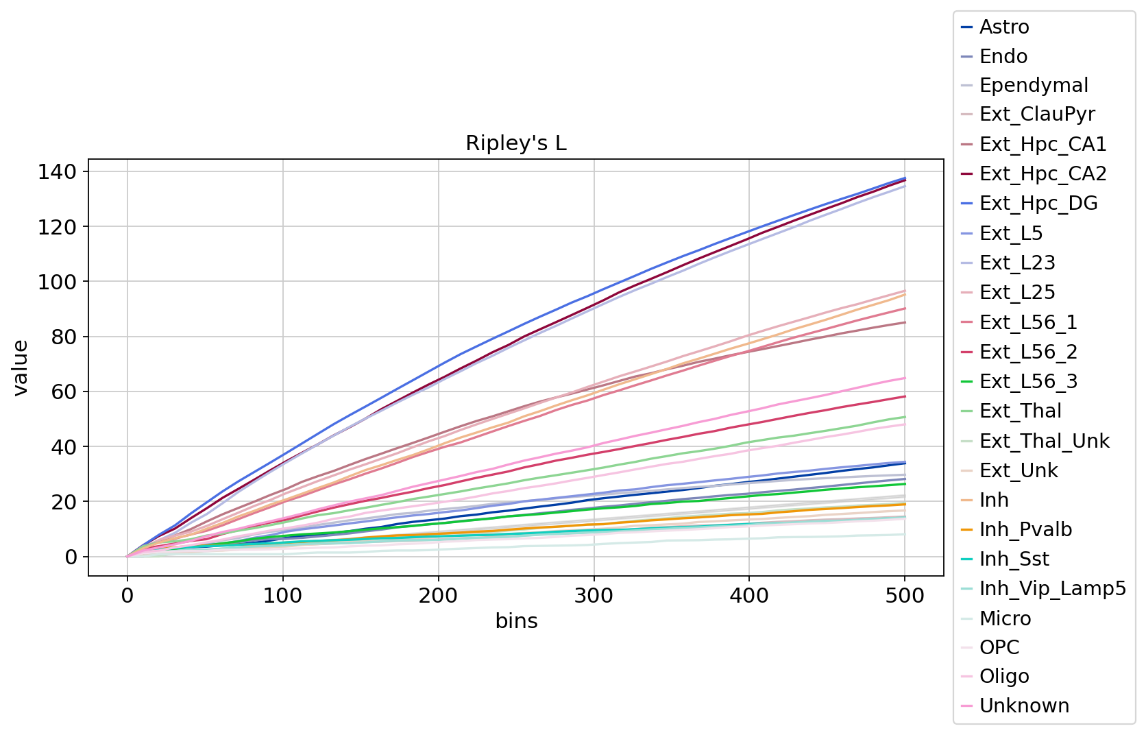

Figure Legend: Change in Ripley's L value as distance increases. X-axis is distance, Y-axis is dispersion level.