SeekSpace 高级分析:基于 Squidpy 的邻域富集与共现分析
执行环境选择 cellcharter-env
Squidpy 是一种用于分析和可视化空间数据的工具。它建立在 scanpy 和 anndata 之上,继承了模块性和可伸缩性。它提供了利用数据的空间坐标以及组织图像(如果有)的分析工具。
分析内容主要包括:
- 邻域富集
- 共现分析
- 高变基因
- 离散程度
数据加载和预处理
基于三个矩阵文件进行读取,另外添加空间位置和细胞注释(可以是任何细胞分群)结果。
adata = sc.read_10x_mtx(
    "/PROJ2/FLOAT/weichendan/seekspace/WTH1092/demo_WTH1092/Outs/WTH1092_filtered_feature_bc_matrix/",
    cache=True
)adatavar: 'gene_ids', 'feature_types'
adata.var_names_make_unique()
sc.pp.filter_cells(adata, min_genes=200)
sc.pp.filter_genes(adata, min_cells=3)

adata.var["mt"] = adata.var_names.str.startswith("mt-")
sc.pp.calculate_qc_metrics(
    adata, qc_vars=["mt"], percent_top=None, log1p=False, inplace=True
)

adata = adata[adata.obs.n_genes_by_counts < 2500, :]
adata = adata[adata.obs.pct_counts_mt < 5, :].copy()

sc.pp.normalize_total(adata, target_sum=1e4)
sc.pp.log1p(adata)
sc.pp.highly_variable_genes(adata, min_mean=0.0125, max_mean=3, min_disp=0.5)

adata.raw = adata

adata = adata[:, adata.var.highly_variable]
sc.pp.regress_out(adata, ["total_counts", "pct_counts_mt"])
sc.pp.scale(adata, max_value=10)

sc.tl.pca(adata, svd_solver="arpack")
sc.pp.neighbors(adata, n_neighbors=10, n_pcs=40)
sc.tl.umap(adata)
sc.tl.tsne(adata)df[key] = c
/PROJ2/FLOAT/weichendan/software/micromamba/envs/cellcharter-env/lib/python3.9/site-packages/tqdm/auto.py:21: TqdmWarning: IProgress not found. Please update jupyter and ipywidgets. See https://ipywidgets.readthedocs.io/en/stable/user_install.html
from .autonotebook import tqdm as notebook_tqdm
adataobs: 'n_genes', 'n_genes_by_counts', 'total_counts', 'total_counts_mt', 'pct_counts_mt'
var: 'gene_ids', 'feature_types', 'n_cells', 'mt', 'n_cells_by_counts', 'mean_counts', 'pct_dropout_by_counts', 'total_counts', 'highly_variable', 'means', 'dispersions', 'dispersions_norm', 'mean', 'std'
uns: 'log1p', 'hvg', 'pca', 'neighbors', 'umap', 'tsne'
obsm: 'X_pca', 'X_umap', 'X_tsne'
varm: 'PCs'
obsp: 'distances', 'connectivities'
spatial_df = pd.read_csv("/PROJ2/FLOAT/weichendan/seekspace/WTH1092/demo_WTH1092/Outs/WTH1092_filtered_feature_bc_matrix/cell_locations.tsv.gz",index_col=0,sep='\t')
spatial_df.columns = ["spatial_1","spatial_2"]
spatial_df = pd.merge(adata.obs, spatial_df, left_index=True, right_index=True)[["spatial_1","spatial_2"]]

adata.obsm["spatial"] = spatial_df.valuesspatial_df| spatial_1 | spatial_2 | |
|---|---|---|
| TTGTGTTATGCAAGAGGTAGTCATACG | 33195 | 11954 |
| TGCGACGATGACGATACCTAAGTACGA | 25664 | 15747 |
| ACCTGAACGAAGGGTCAGCTCTGCTTC | 36614 | 13290 |
| CACTGGGTACGGTCGACCCTAATAACG | 35019 | 10923 |
| AAGATAGCGAAGGAGGGCTAAGTACGA | 42849 | 13006 |
| ... | ... | ... |
| TCAAGCAGCTGTTACCATTCTGCGCTC | 17118 | 14572 |
| ACCCTTGCGAACTCAACGCTCTGCTTC | 34011 | 13369 |
| GTTCTATATGCGGACTGGCTCTGCTTC | 15772 | 12816 |
| TACCGAATACCTCCGACGCTCTGCTTC | 21987 | 16150 |
| AATGAAGGCTCTTGAACAGCGACGGAT | 29200 | 4941 |
22512 rows × 2 columns
cell_anno = pd.read_csv("/PROJ2/FLOAT/weichendan/seekspace/WTH1092/annotation.csv",index_col=0)
cell_anno = cell_anno[["Main_CellType","Sub_CellType"]]

adata.obs = pd.merge(adata.obs,cell_anno,left_index=True,right_index=True)adataobs: 'n_genes', 'n_genes_by_counts', 'total_counts', 'total_counts_mt', 'pct_counts_mt', 'Main_CellType', 'Sub_CellType'
var: 'gene_ids', 'feature_types', 'n_cells', 'mt', 'n_cells_by_counts', 'mean_counts', 'pct_dropout_by_counts', 'total_counts', 'highly_variable', 'means', 'dispersions', 'dispersions_norm', 'mean', 'std'
uns: 'log1p', 'hvg', 'pca', 'neighbors', 'umap', 'tsne'
obsm: 'X_pca', 'X_umap', 'X_tsne', 'spatial'
varm: 'PCs'
obsp: 'distances', 'connectivities'
大群注释结果:
sc.settings.set_figure_params(figsize=(10, 5))
sc.pl.embedding(adata,"spatial",color=["Main_CellType"])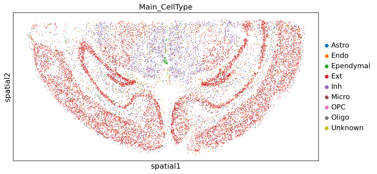
亚群注释结果:
sc.settings.set_figure_params(figsize=(10, 5))
sc.pl.embedding(adata,"spatial",color=["Sub_CellType"])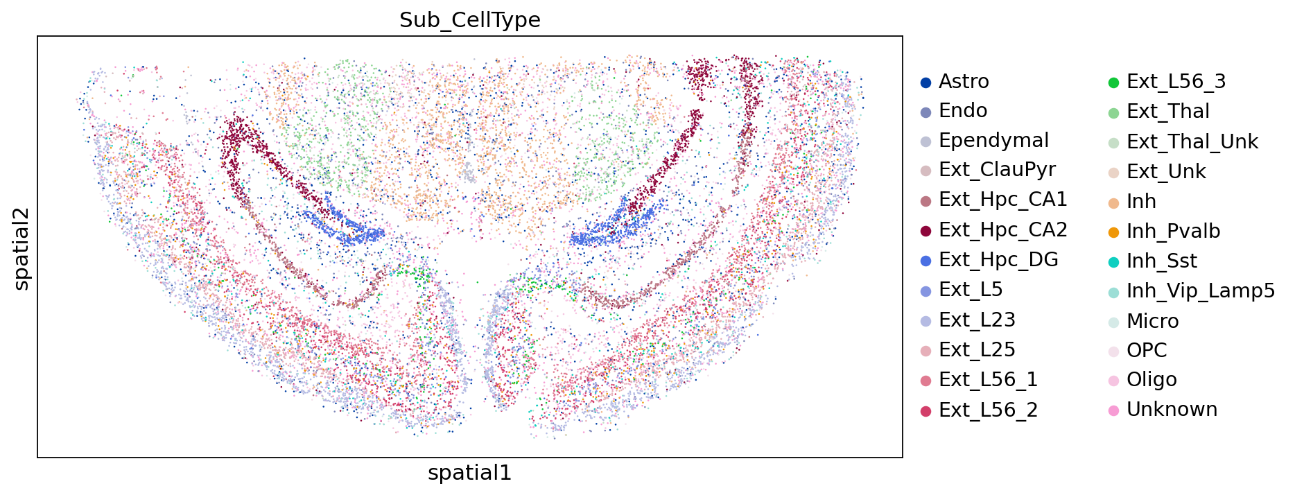
邻域富集
计算邻域富集可以帮助我们识别在整个组织中共享共同邻域结构的细胞 cluster。
简而言之,这是聚类空间接近度的富集分数:如果属于两个不同聚类的细胞通常彼此接近,那么它们将具有高分并且可以被定义为 enriched。另一方面,如果他们相距很远,因此很少是邻居,那么分数就会很低,可以将其定义为 depleted。
sq.gr.spatial_neighbors(adata)
sq.gr.nhood_enrichment(adata, cluster_key="Sub_CellType")adataobs: 'n_genes', 'n_genes_by_counts', 'total_counts', 'total_counts_mt', 'pct_counts_mt', 'Main_CellType', 'Sub_CellType'
var: 'gene_ids', 'feature_types', 'n_cells', 'mt', 'n_cells_by_counts', 'mean_counts', 'pct_dropout_by_counts', 'total_counts', 'highly_variable', 'means', 'dispersions', 'dispersions_norm', 'mean', 'std'
uns: 'log1p', 'hvg', 'pca', 'neighbors', 'umap', 'tsne', 'Main_CellType_colors', 'Sub_CellType_colors', 'spatial_neighbors', 'Sub_CellType_nhood_enrichment'
obsm: 'X_pca', 'X_umap', 'X_tsne', 'spatial'
varm: 'PCs'
obsp: 'distances', 'connectivities', 'spatial_connectivities', 'spatial_distances'
sq.pl.nhood_enrichment(adata, cluster_key="Sub_CellType", figsize=(5, 10))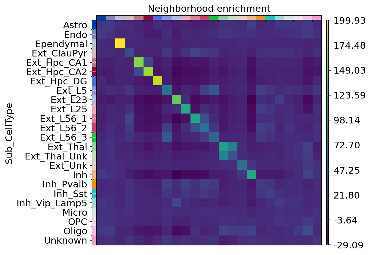
图注:空间坐标中细胞簇之间的邻域富集分析。
空间维度共现分析
除了邻域富集得分外,我们还可以在空间维度上可视化集群共存。这是对上述分析的类似分析,但它不在数据矩阵上运行,而是在原始空间坐标上运行。
sq.gr.co_occurrence(adata, cluster_key="Sub_CellType")adataobs: 'n_genes', 'n_genes_by_counts', 'total_counts', 'total_counts_mt', 'pct_counts_mt', 'Main_CellType', 'Sub_CellType'
var: 'gene_ids', 'feature_types', 'n_cells', 'mt', 'n_cells_by_counts', 'mean_counts', 'pct_dropout_by_counts', 'total_counts', 'highly_variable', 'means', 'dispersions', 'dispersions_norm', 'mean', 'std'
uns: 'log1p', 'hvg', 'pca', 'neighbors', 'umap', 'tsne', 'Main_CellType_colors', 'Sub_CellType_colors', 'spatial_neighbors', 'Sub_CellType_nhood_enrichment', 'Sub_CellType_co_occurrence'
obsm: 'X_pca', 'X_umap', 'X_tsne', 'spatial'
varm: 'PCs'
obsp: 'distances', 'connectivities', 'spatial_connectivities', 'spatial_distances'
np.unique(adata.obs['Sub_CellType'])'Ext_Hpc_CA2', 'Ext_Hpc_DG', 'Ext_L23', 'Ext_L25', 'Ext_L5',
'Ext_L56_1', 'Ext_L56_2', 'Ext_L56_3', 'Ext_Thal', 'Ext_Thal_Unk',
'Ext_Unk', 'Inh', 'Inh_Pvalb', 'Inh_Sst', 'Inh_Vip_Lamp5', 'Micro',
'OPC', 'Oligo', 'Unknown'], dtype=object)
import matplotlib.pyplot as plt
sq.pl.co_occurrence(
    adata,
    cluster_key="Sub_CellType",
    clusters="Astro",
    figsize=(10, 4)
)
# 获取当前 axes 上的图例(如果有)
legend = plt.gca().get_legend()

if legend is not None:
    # 获取图例的句柄和标签
    handles, labels = legend.legend_handles, [t.get_text() for t in legend.texts]
    # 移除旧的图例
    legend.remove()
    # 添加新的图例,并设置 ncol=2
    plt.legend(
        handles=handles,
        labels=labels,
        loc='center left',  # 或者指定位置,如 'upper right'
        bbox_to_anchor=(1, 0.5), # 放在 axes 的右侧(1 表示 axes 右边界之外)
        ncol=2,       # 设置为两列
    )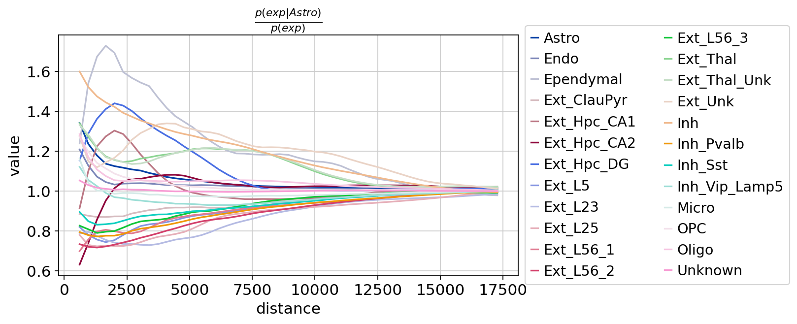
图注:每个细胞的聚类共现评分。在组织中,随着距离阈值的增加,每个细胞的聚类共现评分逐渐变化。横轴是距离,纵轴是共现评分
空间高变基因 Moran’s I
空间高变基因(Spatially Variable Genes, SVGs)是指在空间转录组数据中,在不同空间位置(如组织切片中的不同区域、发育过程中的不同结构域等)表达模式具有显著变异的基因。这些基因通常与组织微环境、细胞类型分布、发育梯度、病理状态等密切相关,是解析空间组织结构和功能异质性的关键切入点。 接下来可以找到显示空间模式的基因,在这里,我们提供了一种基于著名的 Moran's I 统计数据的简单方法。
genes = adata[:, adata.var.highly_variable].var_names.values[:1000]
sq.gr.spatial_autocorr(
    adata,
    mode="moran",
    genes=genes,
    n_perms=100,
    n_jobs=1,
)adataobs: 'n_genes', 'n_genes_by_counts', 'total_counts', 'total_counts_mt', 'pct_counts_mt', 'Main_CellType', 'Sub_CellType'
var: 'gene_ids', 'feature_types', 'n_cells', 'mt', 'n_cells_by_counts', 'mean_counts', 'pct_dropout_by_counts', 'total_counts', 'highly_variable', 'means', 'dispersions', 'dispersions_norm', 'mean', 'std'
uns: 'log1p', 'hvg', 'pca', 'neighbors', 'umap', 'tsne', 'Main_CellType_colors', 'Sub_CellType_colors', 'spatial_neighbors', 'Sub_CellType_nhood_enrichment', 'Sub_CellType_co_occurrence', 'moranI'
obsm: 'X_pca', 'X_umap', 'X_tsne', 'spatial'
varm: 'PCs'
obsp: 'distances', 'connectivities', 'spatial_connectivities', 'spatial_distances'
高变基因评估结果:
adata.uns["moranI"].head(10)| I | pval_norm | var_norm | pval_z_sim | pval_sim | var_sim | pval_norm_fdr_bh | pval_z_sim_fdr_bh | pval_sim_fdr_bh | |
|---|---|---|---|---|---|---|---|---|---|
| Wfdc2 | 0.469195 | 0.0 | 0.000013 | 0.0 | 0.009901 | 0.000021 | 0.0 | 0.0 | 0.025987 |
| Dpp10 | 0.339641 | 0.0 | 0.000013 | 0.0 | 0.009901 | 0.000017 | 0.0 | 0.0 | 0.025987 |
| Tshz2 | 0.315615 | 0.0 | 0.000013 | 0.0 | 0.009901 | 0.000023 | 0.0 | 0.0 | 0.025987 |
| Hpca | 0.304144 | 0.0 | 0.000013 | 0.0 | 0.009901 | 0.000017 | 0.0 | 0.0 | 0.025987 |
| Spag17 | 0.298851 | 0.0 | 0.000013 | 0.0 | 0.009901 | 0.000023 | 0.0 | 0.0 | 0.025987 |
| Fibcd1 | 0.298201 | 0.0 | 0.000013 | 0.0 | 0.009901 | 0.000024 | 0.0 | 0.0 | 0.025987 |
| Tmem212 | 0.261650 | 0.0 | 0.000013 | 0.0 | 0.009901 | 0.000011 | 0.0 | 0.0 | 0.025987 |
| Ccdc146 | 0.261100 | 0.0 | 0.000013 | 0.0 | 0.009901 | 0.000021 | 0.0 | 0.0 | 0.025987 |
| Synpo2 | 0.240745 | 0.0 | 0.000013 | 0.0 | 0.009901 | 0.000014 | 0.0 | 0.0 | 0.025987 |
| Camk2n1 | 0.233325 | 0.0 | 0.000013 | 0.0 | 0.009901 | 0.000016 | 0.0 | 0.0 | 0.025987 |
top5 高变基因在组织切片上的空间表达情况:
adata.uns["moranI"].index[0:5]#sq.pl.spatial_scatter(adata, color=adata.uns["moranI"].index[0:5])
sc.pl.embedding(adata,"spatial",color=adata.uns["moranI"].index[0:4])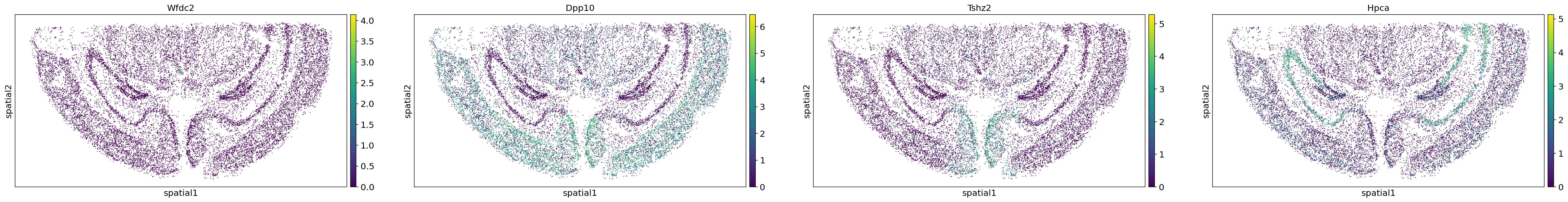
图注:通过 Moran‘s I 空间自相关分析计算得出的四个空间变异基因(Wfdc2、Dpp10、Tshz2 和 Hpca)的表达情况。这些基因似乎呈现出不同的模式特征,并对不同细胞类型具有特异性表达。
细胞分群在空间上的离散程度
除了邻域富集评分外,我们还可以通过 Ripley 统计数据进一步研究组织中细胞类型的空间组织。Ripley 的统计数据允许分析人员评估离散注释(例如细胞类型)在感兴趣的区域上是聚集的,分散的还是随机分布的。
mode = "L"
sq.gr.ripley(adata, cluster_key="Sub_CellType", mode=mode, max_dist=500)adataobs: 'n_genes', 'n_genes_by_counts', 'total_counts', 'total_counts_mt', 'pct_counts_mt', 'Main_CellType', 'Sub_CellType'
var: 'gene_ids', 'feature_types', 'n_cells', 'mt', 'n_cells_by_counts', 'mean_counts', 'pct_dropout_by_counts', 'total_counts', 'highly_variable', 'means', 'dispersions', 'dispersions_norm', 'mean', 'std'
uns: 'log1p', 'hvg', 'pca', 'neighbors', 'umap', 'tsne', 'Main_CellType_colors', 'Sub_CellType_colors', 'spatial_neighbors', 'Sub_CellType_nhood_enrichment', 'Sub_CellType_co_occurrence', 'moranI', 'Sub_CellType_ripley_L'
obsm: 'X_pca', 'X_umap', 'X_tsne', 'spatial'
varm: 'PCs'
obsp: 'distances', 'connectivities', 'spatial_connectivities', 'spatial_distances'
adata.uns["Sub_CellType_ripley_L"]0 0.000000 Astro 0.000000
1 10.204082 Astro 1.637580
2 20.408163 Astro 2.315888
3 30.612245 Astro 3.171160
4 40.816327 Astro 3.375957
... ... ... ...n 1195 459.183673 Unknown 60.034669
1196 469.387755 Unknown 61.332776
1197 479.591837 Unknown 62.609327
1198 489.795918 Unknown 63.813106
1199 500.000000 Unknown 64.839684
[1200 rows x 3 columns],
'sims_stat': bins simulations stats
0 0.000000 0 0.000000
1 10.204082 0 0.000000
2 20.408163 0 0.818790
3 30.612245 0 1.157944
4 40.816327 0 1.157944
... ... ... ...n 4995 459.183673 99 20.486117
4996 469.387755 99 20.713929
4997 479.591837 99 21.209662
4998 489.795918 99 21.694070
4999 500.000000 99 22.137633
[5000 rows x 3 columns],
'bins': array([ 0. , 10.20408163, 20.40816327, 30.6122449 ,
40.81632653, 51.02040816, 61.2244898 , 71.42857143,
81.63265306, 91.83673469, 102.04081633, 112.24489796,
122.44897959, 132.65306122, 142.85714286, 153.06122449,
163.26530612, 173.46938776, 183.67346939, 193.87755102,
204.08163265, 214.28571429, 224.48979592, 234.69387755,
244.89795918, 255.10204082, 265.30612245, 275.51020408,
285.71428571, 295.91836735, 306.12244898, 316.32653061,
326.53061224, 336.73469388, 346.93877551, 357.14285714,
367.34693878, 377.55102041, 387.75510204, 397.95918367,
408.16326531, 418.36734694, 428.57142857, 438.7755102 ,
448.97959184, 459.18367347, 469.3877551 , 479.59183673,
489.79591837, 500. ]),
'pvalues': array([[0. , 0.00990099, 0.00990099, ..., 0.00990099, 0.00990099,
0.00990099],
[0. , 0.00990099, 0.00990099, ..., 0.00990099, 0.00990099,
0.00990099],
[0. , 0. , 0.32673267, ..., 0.00990099, 0.00990099,
0.00990099],
...,
[0. , 0.06930693, 0.05940594, ..., 0. , 0. ,
0. ],
[0. , 0.00990099, 0.00990099, ..., 0.00990099, 0.00990099,
0.00990099],
[0. , 0.00990099, 0.00990099, ..., 0.00990099, 0.00990099,
0.00990099]])}
sq.pl.ripley(adata, cluster_key="Sub_CellType", mode=mode)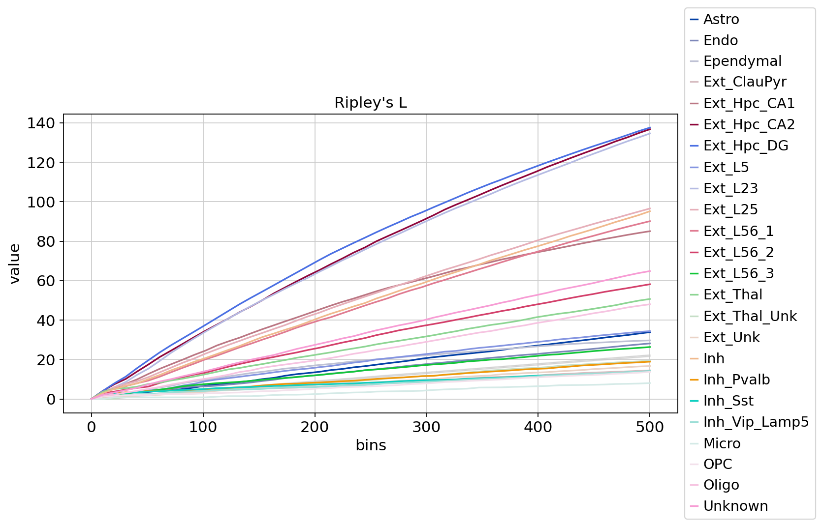
图注:随着距离的增加 Ripley’s L 值的变化。横轴是距离,纵轴是离散值的高低。