stLearn Advanced Spatial Transcriptomics Analysis: Ligand-Receptor Interaction Hotspot Identification

Author: SeekGene

Time: 18 min

Words: 3.5k words

Updated: 2026-02-28

Reads: 0 times

Spatial-seq Analysis Guide Notebooks Cell Communication Analysis

Background Introduction

stLearn uses ligand-receptor co-expression information between neighboring spots and cell type diversity to calculate ligand-receptor (LR) scores. It can identify hotspot regions within a given tissue where LR interactions between cell types are more likely to occur compared to the spatial distribution of random non-interacting gene pairs (i.e., considering communication between neighboring cells and LR co-expression).

stLearn Calculation Results

import stlearn as st
import numpy as np
import pandas as pd
# matplotlib version 3.5.3, higher versions conflict with stlearn
import matplotlib.pyplot as plt
import matplotlib.image as mpimg
import scanpy as sc
import re
import warnings
from PIL import Image
import os

output

/jp_envs/envs/stlearn/lib/python3.9/site-packages/stlearn/tools/microenv/cci/het.py:192: NumbaDeprecationWarning: The keyword argument 'nopython=False' was supplied. From Numba 0.59.0 the default is being changed to True and use of 'nopython=False' will raise a warning as the argument will have no effect. See https://numba.readthedocs.io/en/stable/reference/deprecation.html#deprecation-of-object-mode-fall-back-behaviour-when-using-jit for details.
@jit(parallel=True, nopython=False)

stLearn Cell Communication Module Input Parameters:

• SAMple_name: Sample name
• meta_path: Metadata file path
• spot_diameter_fullres: Size of cell/spot, related to spatial distance range in analysis steps
• species: Species, must be "human" or "mouse"
• meta_celltype_colums_name: Set column name for cell types in adata object obs

sample_name = "N1"
meta_path = "../../data/AY1748480899609/meta.tsv"
spot_diameter_fullres = 50
species = "human"
meta_celltype_colums_name = "CellAnnotation"

• Read SeekSpace data and perform normalization, dimensionality reduction, clustering (input.rds needs to be converted to matrix file beforehand)

adata = sc.read_10x_mtx("./filtered_feature_bc_matrix/")
spatial = pd.read_csv('./filtered_feature_bc_matrix/cell_locations.tsv',sep="\t",index_col=0)
spatial = spatial.loc[:,("x","y")]
selected_rows = spatial.loc[spatial.index.isin(adata.obs_names)]
selected_rows.columns = ["imagecol","imagerow"]
selected_rows = selected_rows.reindex(adata.obs_names)
selected_rows = selected_rows*0.265385
a = st.create_stlearn(count=adata.to_df(),spatial=selected_rows,library_id=sample_name, scale=1,spot_diameter_fullres=spot_diameter_fullres)
a.layers["raw_count"] = a.X
# Preprocessing
st.pp.normalize_total(a)
st.pp.log1p(a)
# Keep raw data
a.raw = a
st.pp.scale(a)
st.em.run_pca(a,n_comps=50,random_state=0)
st.pp.neighbors(a,n_neighbors=25,use_rep='X_pca',random_state=0)
st.tl.clustering.louvain(a,random_state=0)
sc.tl.umap(a)

output

Normalization step is finished in adata.X
Log transformation step is finished in adata.X
Scale step is finished in adata.X
PCA is done! Generated in adata.obsm['X_pca'], adata.uns['pca'] and adata.varm['PCs']


/jp_envs/envs/stlearn/lib/python3.9/site-packages/tqdm/auto.py:21: TqdmWarning: IProgress not found. Please update jupyter and ipywidgets. See https://ipywidgets.readthedocs.io/en/stable/user_install.html
from .autonotebook import tqdm as notebook_tqdm
2025-08-28 17:39:53.325920: I tensorflow/core/platform/cpu_feature_guard.cc:193] This TensorFlow binary is optimized with oneAPI Deep Neural Network Library (oneDNN) to use the following CPU instructions in performance-critical operations: SSE4.1 SSE4.2 AVX AVX2 AVX512F AVX512_VNNI AVX512_BF16 AVX_VNNI AMX_TILE AMX_INT8 AMX_BF16 FMA
To enable them in other operations, rebuild TensorFlow with the appropriate compiler flags.
2025-08-28 17:39:55.109291: I tensorflow/core/util/port.cc:104] oneDNN custom operations are on. You may see slightly different numerical results due to floating-point round-off errors from different computation orders. To turn them off, set the environment variable \`TF_ENABLE_ONEDNN_OPTS=0\`.


Created k-Nearest-Neighbor graph in adata.uns['neighbors']
Applying Louvain cluster ...n Louvain cluster is done! The labels are stored in adata.obs['louvain']

Add annotated cell types to adata object

cluster_name = "celltype"
celltype = pd.read_csv(meta_path,index_col=0,sep = "\t")
celltype = celltype.loc[a.obs.index]
a.obs[cluster_name] = celltype[meta_celltype_colums_name]
a.obs[cluster_name] = a.obs[cluster_name].astype('category')

• Divide spatial slice into length n_, width n_
  Note: To save time, divide the spatial slice into n×n grids (equivalent to bins) for subsequent cell communication analysis (grid_step=True); if you want to calculate cell communication at single-cell level, skip this step (grid_step=False)

grid_step=False
if grid_step:
    #n_ = 125
    print(f'{n_grid} by {n_grid} has this many spots:\n', n_grid*n_grid)
    a = st.tl.cci.grid(a,n_row=n_grid, n_col=n_grid, use_label = cluster_name)
    print(a.shape)

• Load ligand-receptor database, calculate significance of LR expression

lrs = st.tl.cci.load_lrs(['connectomeDB2020_lit'], species=species)



st.tl.cci.run(a, lrs,
                  min_spots = 20, #Filter out any LR pairs with no scores for less than min_spots
                  distance=None, # None defaults to spot+immediate neighbours; distance=0 for within-spot mode
                  n_pairs=10000, # Number of random pairs to generate; low as example, recommend ~10,000
                  n_cpus=12, # Number of CPUs for parallel. If None, detects & use all available.
                  )

output

Calculating neighbours...n 112 spots with no neighbours, 14 median spot neighbours.
Spot neighbour indices stored in adata.obsm['spot_neighbours'] & adata.obsm['spot_neigh_bcs'].
Altogether 1483 valid L-R pairs


Generating backgrounds & testing each LR pair...: 1%|▏ [ time left: 2:49:41 ]

Ligand-Receptor Expression Significance Results

lr_info = a.uns['lr_summary']

lr_info

	n_spots	n_spots_sig	n_spots_sig_pval
THBS1_LRP1	3185	1505	1870
PTPRK_PTPRK	2622	1471	2013
A2M_LRP1	3078	1412	1845
VEGFA_GPC1	3258	1260	1897
PTPRM_PTPRM	2731	1203	1669
...	...	...	...
FGF3_FGFRL1	27	12	24
GHRH_VIPR1	24	12	24
INHBC_ACVR2A	25	12	20
NPPC_NPR3	21	12	20
BMP10_BMPR1A	21	6	13

1483 rows × 3 columns

- Rows: Ligand-Receptor Pairs  
- Column 1 n_spot: Total number of cells/spots with LR interactions without pval filtering  
- Column 2 n_spots_sig: Number of cells/spots with significant LR interactions after corrected pval filtering  
- Column 3 n_spots_sig_pval: Number of cells/spots with LR interactions after filtering by set pval

st.tl.cci.adj_pvals(a, correct_axis='spot',
                   pval_adj_cutoff=0.05, adj_method='fdr_bh')

output

Updated adata.uns[lr_summary]
Updated adata.obsm[lr_scores]
Updated adata.obsm[lr_sig_scores]
Updated adata.obsm[p_vals]
Updated adata.obsm[p_adjs]
Updated adata.obsm[-log10(p_adjs)]

Ligand-Receptor Diagnostic Plot

A key aspect of LR analysis is controlling for LR expression levels and frequency when identifying significant hotspots. Therefore, diagnostic plots should show little correlation between LR hotspots and expression levels/frequency. The following diagnostics help check this; if not, it suggests a larger number of Permutations may be needed.

st.pl.lr_diagnostics(a, show=False,figsize=(15,5))

output

(Figure size 1500x500 with 2 Axes,
array([,
],
dtype=object))

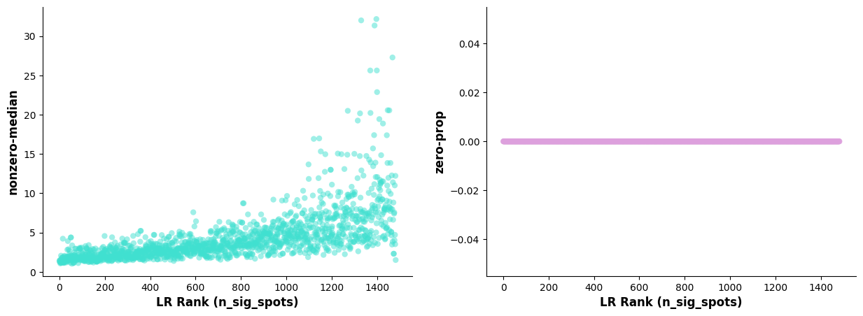
* **Left Plot:** X-axis is sorted LR pairs by n_spots_sig; Y-axis is median expression of LR pairs (non-zero).
* **Right Plot:** X-axis is sorted LR pairs by n_spots_sig; Y-axis is proportion of cells with zero expression of LR pairs.

Scatter Plot of Significant Interacting Ligand-Receptors

#st.pl.lr_summary(a, n_top=500,show=False)
st.pl.lr_summary(a, n_top=50, show=False,figsize=(10,3))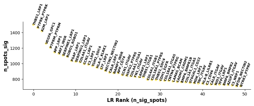

output

Plot based on lr_summary results: Showing top 50 LR pairs. X-axis represents LR pairs sorted by n_spots_sig; Y-axis represents number of cells/spots with significant LR interaction after corrected pval filtering.

Bar Plot of Significant Interacting Ligand-Receptors

st.pl.lr_n_spots(a, n_top=50,max_text=100,show=False,figsize=(11, 3))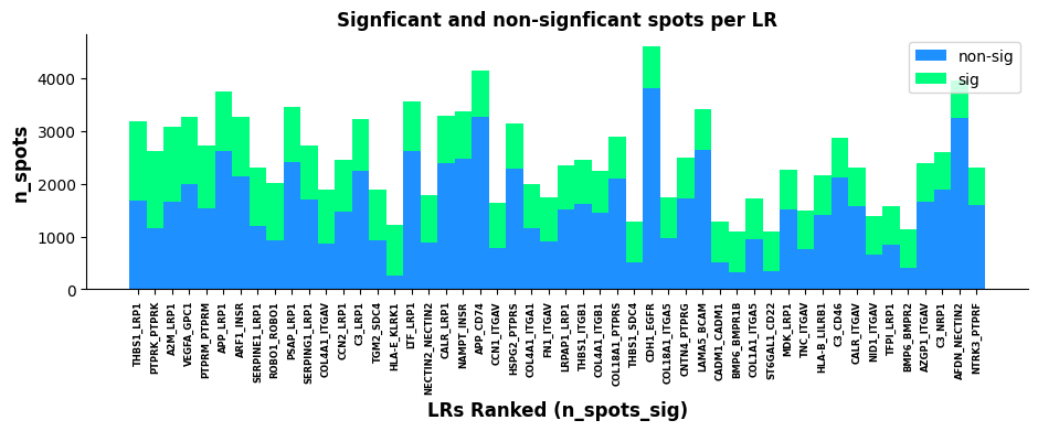

output

(Figure size 1100x300 with 1 Axes,
)

Plot based on lr_summary results: Showing top 500 and top 50 LR pairs. X-axis represents LR pairs sorted by n_spots_sig; Y-axis represents total number of cells/spots with LR interaction (unfiltered by pval); Green and blue represent significant and non-significant LR pairs respectively.

LR Statistics Visualization

Visualize hotspots of significant LR pair co-expression to roughly see areas where interactions of interest are concentrated.

lr_scores = pd.DataFrame(a.obsm["lr_scores"])
lr_scores.columns = lr_info.index
lr_scores.index = a.obs.index

p_vals = pd.DataFrame(a.obsm["p_vals"])
p_vals.columns = lr_info.index
p_vals.index = a.obs.index

p_adjs = pd.DataFrame(a.obsm["p_adjs"])
p_adjs.columns = lr_info.index
p_adjs.index = a.obs.index

log10_p_adjs = pd.DataFrame(a.obsm["-log10(p_adjs)"])
log10_p_adjs.columns = lr_info.index
log10_p_adjs.index = a.obs.index

spatial["LR_score"] = list(lr_scores["THBS1_LRP1"])
spatial["p_vals"] = list(p_vals["THBS1_LRP1"])
spatial["p_adjs"] = list(p_adjs["THBS1_LRP1"])
spatial["-log10(p_adjs)"] = list(log10_p_adjs["THBS1_LRP1"])

spatial

	x	y	LR_score	p_vals	p_adjs	-log10(p_adjs)
Barcode
AACCTGAGCTAGATTAGAGCGACGGAT_1	16898	9879	0.000000	1.0000	1.00000	-0.000000
AAGACAAGCTGATACCTGCTCTGCTTC_1	40296	7851	1.194025	0.0111	0.01353	1.868702
AAGTACCCGAGATAAACAAGGCACTAT_1	31685	6429	-0.203235	1.0000	1.00000	-0.000000
AGAAGCGGCTTCCGATACCTAATAACG_1	16767	17485	-0.460579	1.0000	1.00000	-0.000000
AGACTCAATGAATGCACTTCTGCGCTC_1	11746	14166	-0.203235	1.0000	1.00000	-0.000000
...	...	...	...	...	...	...
TCCGATCCGAAGGAGGGAAGGCACTAT_1	30882	9777	-0.314717	1.0000	1.00000	-0.000000
TGAGGAGGCTCGACAAGTTCTGCGCTC_1	45879	10249	-0.004137	1.0000	1.00000	-0.000000
AGGTCTACGATGTGGAGGCTCTGCTTC_1	54295	6672	0.000000	1.0000	1.00000	-0.000000
TTCCTTCATGCGCTTCGAAGGCACTAT_1	30565	10833	0.000000	1.0000	1.00000	-0.000000
CATAAGCGCTACTCAACGGACTGTGGA_1	16847	944	-0.196527	1.0000	1.00000	-0.000000

20820 rows × 6 columns

# Read spatial HE or DAPI
background_image = mpimg.imread('filtered_feature_bc_matrix/N1_expression.png')

# Create a new figure
fig, ax = plt.subplots(figsize=(12, 8))

# Display background image
ax.imshow(background_image, extent=[0, 55050, 0, 19906], aspect='auto')

# Select numerical column for color gradient (please modify column name based on your data)
# E.g., 'expression_level', 'score', 'intensity', etc.
value_column = 'LR_score'  # Please replace with actual numerical column name

# Create colormap
# Choose different colormaps: 'viridis', 'plasma', 'inferno', 'magma', 'coolwarm', 'RdBu_r', etc.
cmap = plt.cm.viridis
norm = plt.Normalize(vmin=spatial[value_column].min(), 
                    vmax=spatial[value_column].max())

# Create scatter plot, color by numerical column
scatter = ax.scatter(spatial['x'], spatial['y'], 
                    c=spatial[value_column], 
                    cmap=cmap, norm=norm, 
                    alpha=0.7, s=15, edgecolors='none')

# Add colorbar
cbar = plt.colorbar(scatter, ax=ax, shrink=0.8)
cbar.set_label(value_column, fontsize=12)

# Add labels and title
ax.set_xlabel('Spatial_1', fontsize=12)
ax.set_ylabel('Spatial_2', fontsize=12)
ax.set_title(f'THBS1_LRP1 {value_column}', fontsize=14)

# Remove axis ticks (optional, for better aesthetics)
ax.set_xticks([])
ax.set_yticks([])
ax.set_aspect("equal")
# Display plot
plt.tight_layout()
plt.show()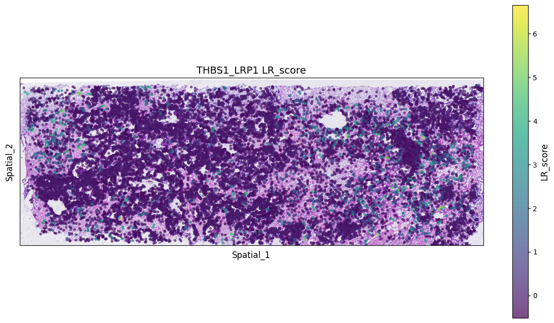

# Read spatial HE or DAPI
background_image = mpimg.imread('filtered_feature_bc_matrix/N1_expression.png')

# Create a new figure
fig, ax = plt.subplots(figsize=(12, 8))

# Display background image
ax.imshow(background_image, extent=[0, 55050, 0, 19906], aspect='auto')

# Select numerical column for color gradient (please modify column name based on your data)
# E.g., 'expression_level', 'score', 'intensity', etc.
value_column = 'p_adjs'  # Please replace with actual numerical column name

# Create colormap
# Choose different colormaps: 'viridis', 'plasma', 'inferno', 'magma', 'coolwarm', 'RdBu_r', etc.
cmap = plt.cm.viridis
norm = plt.Normalize(vmin=spatial[value_column].min(), 
                    vmax=spatial[value_column].max())

# Create scatter plot, color by numerical column
scatter = ax.scatter(spatial['x'], spatial['y'], 
                    c=spatial[value_column], 
                    cmap=cmap, norm=norm, 
                    alpha=0.7, s=15, edgecolors='none')

# Add colorbar
cbar = plt.colorbar(scatter, ax=ax, shrink=0.8)
cbar.set_label(value_column, fontsize=12)

# Add labels and title
ax.set_xlabel('Spatial_1', fontsize=12)
ax.set_ylabel('Spatial_2', fontsize=12)
ax.set_title(f'THBS1_LRP1 {value_column}', fontsize=14)

# Remove axis ticks (optional, for better aesthetics)
ax.set_xticks([])
ax.set_yticks([])
ax.set_aspect("equal")
# Display plot
plt.tight_layout()
plt.show()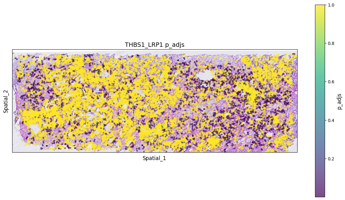

• Predict Significant Interacting Cell Types

st.tl.cci.run_cci(a, cluster_name, # Spot cell information either in data.obs or data.uns
                  min_spots=3, # Minimum number of spots for LR to be tested.
                  sig_spots=True, # Only consider neighbourhoods of spots which had significant LR scores.
                  n_perms=1000, # Permutations of cell information to get background, recommend ~1000
                  n_cpus=16
                 )

output

Getting cached neighbourhood information...n Getting information for CCI counting...n

Counting celltype-celltype interactions per LR and permutating 1000 times.: 0%| [ time left: 31:03:47 ]

Cell Type Diagnostic Plot

Check correlation between LR interaction and cell counts of cell types. If permutations are sufficient, charts below should show little or no correlation; otherwise, increase n_perms.

st.pl.cci_check(a, cluster_name,show=False,figsize=(10,4),cell_label_size=10,axis_text_size=12)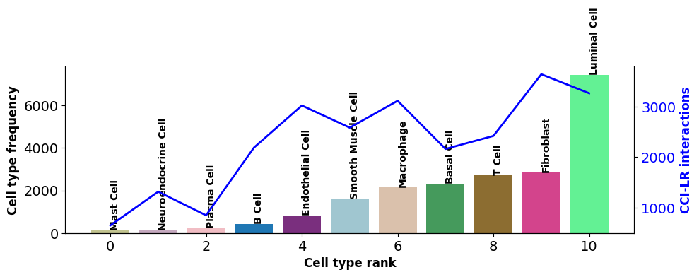

output

(Figure size 1000x400 with 2 Axes,
,
)

X-axis represents cell types; Bar chart left Y-axis represents cell type count; Line chart right Y-axis represents number of interacting LRs for cell type.

CCI Network Plot

st.pl.ccinet_plot(a, cluster_name, return_pos=True,pad=0.3,node_size_exp=0.8)


lr_pair = a.uns['lr_summary'].index.values[0:3]
st.pl.ccinet_plot(a, cluster_name, lr_pair[1], min_counts=2,pad=0.3,node_size_exp=0.8)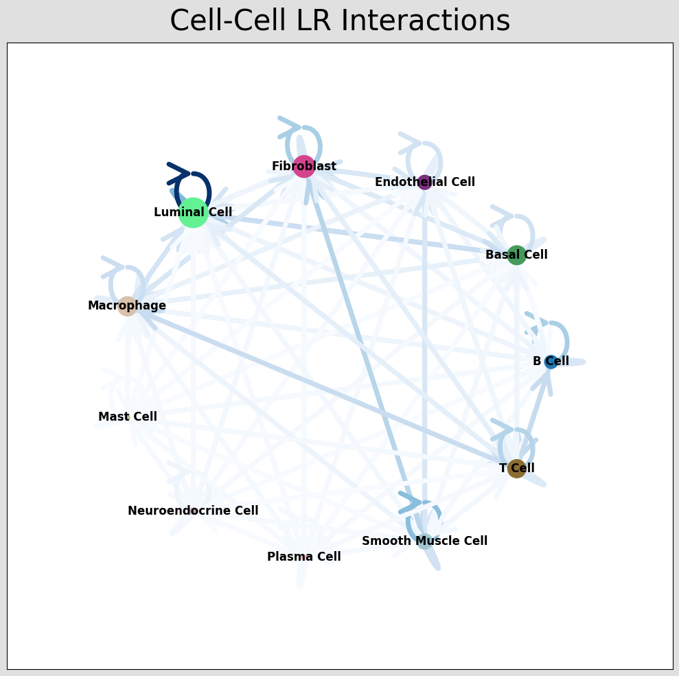

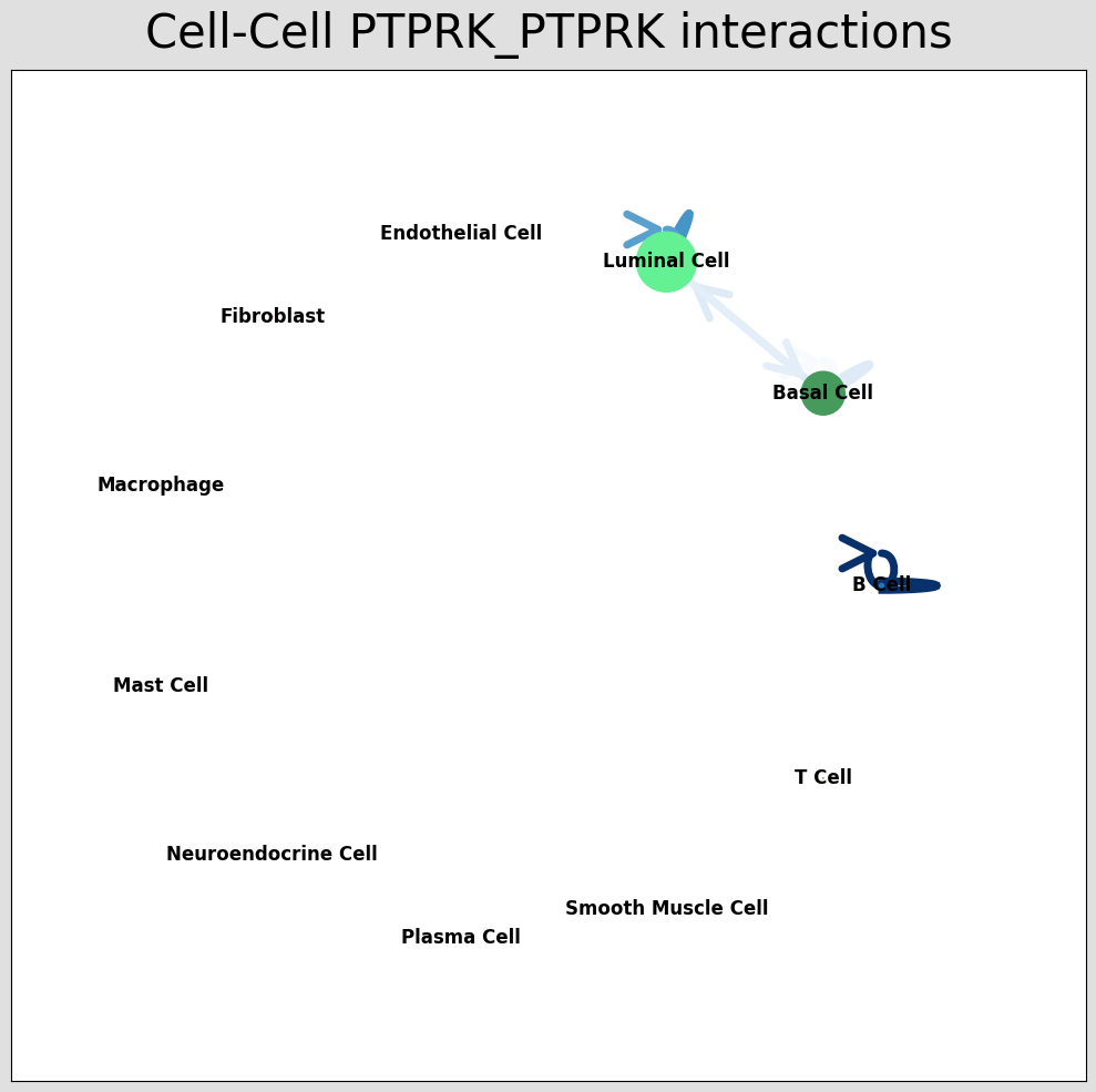
CCI network plot shows cell type interactions for corresponding LR pairs, plotted via per_lr_cci_* results. Each color represents a cell type; lines pointing from a cell type to itself or others represent interactions; line color intensity represents interaction strength.

CCI Chord Diagram

st.pl.lr_chord_plot(a, cluster_name,show=False)


st.pl.lr_chord_plot(a, cluster_name,show=False,lr=lr_pair[1])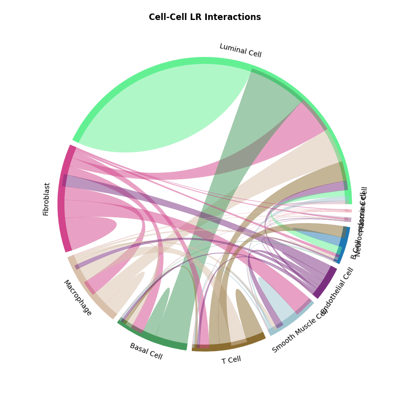

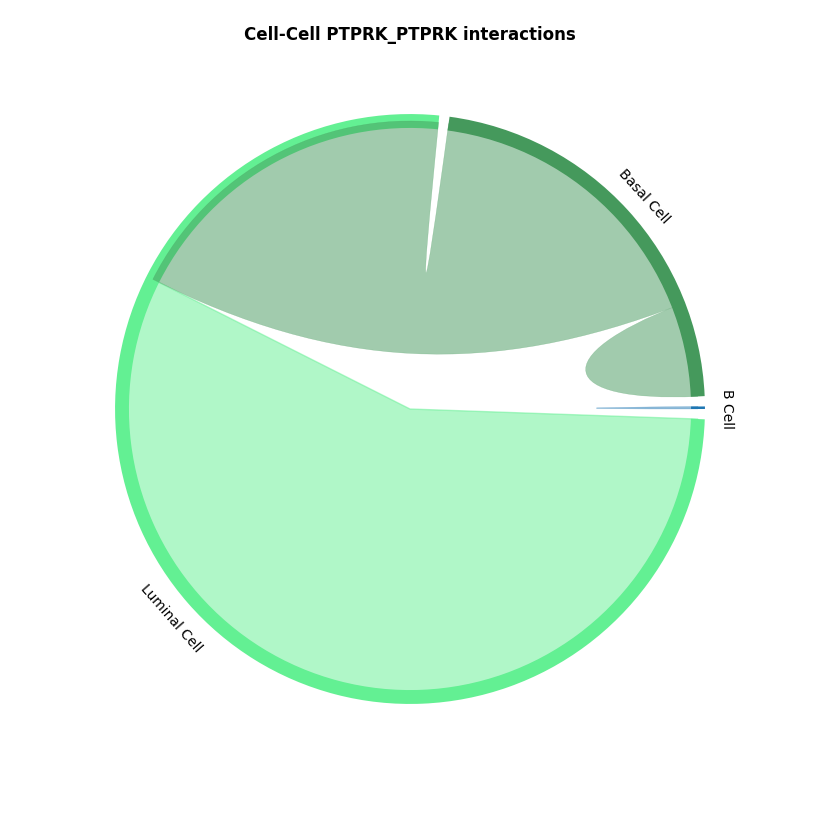
output

(Figure size 800x800 with 1 Axes, Axes:)

CCI chord diagram shows cell type interactions for corresponding LR pairs, plotted via per_lr_cci_* results. Each color represents a cell type; chord width represents interaction strength, wider chords mean stronger interactions.

CCI Heatmap

st.pl.lr_cci_map(a, cluster_name, lrs=None, min_total=100, figsize=(20,4),show=False)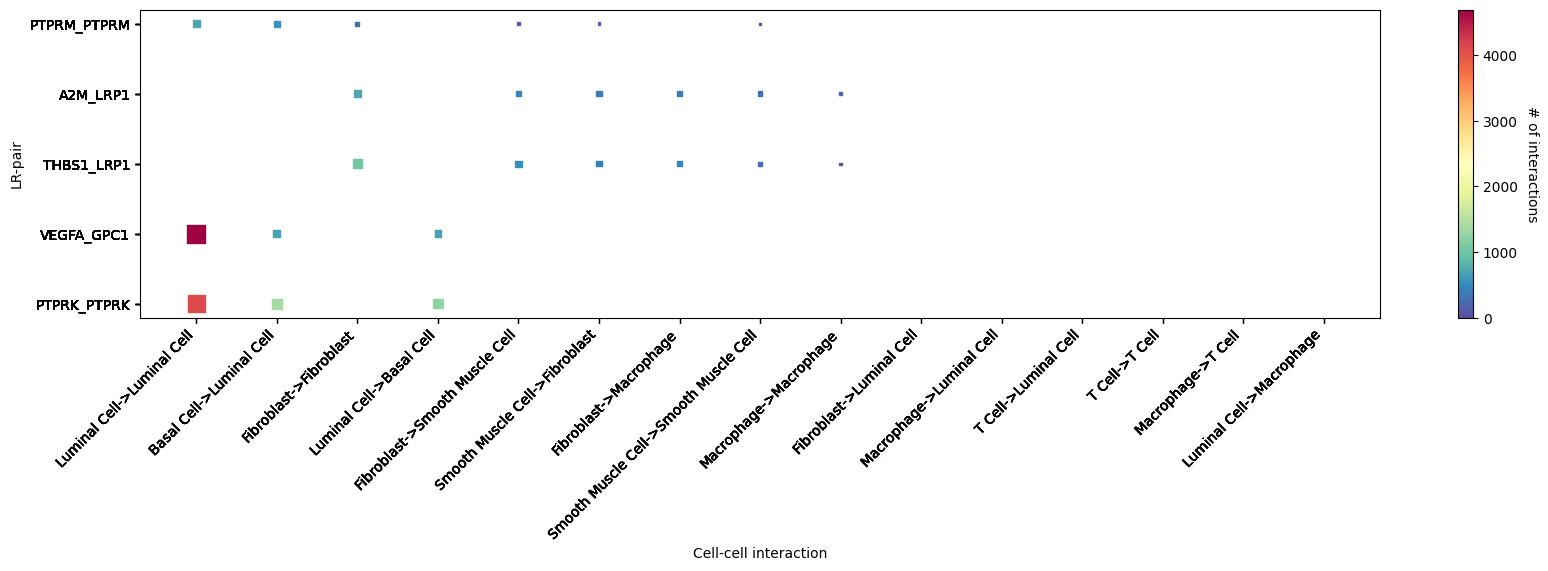

output

CCI heatmap shows LR interactions corresponding to cell types. X-axis represents interacting cell types; Y-axis represents interacting LRs; color represents interaction strength, redder means stronger. Shows top 5 significantly interacting LR pairs.

st.pl.cci_map(a, cluster_name,show=False,figsize=(5,4))


st.pl.cci_map(a, cluster_name, lr=lr_pair[1],show=False,figsize=(5,4))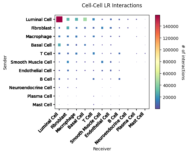

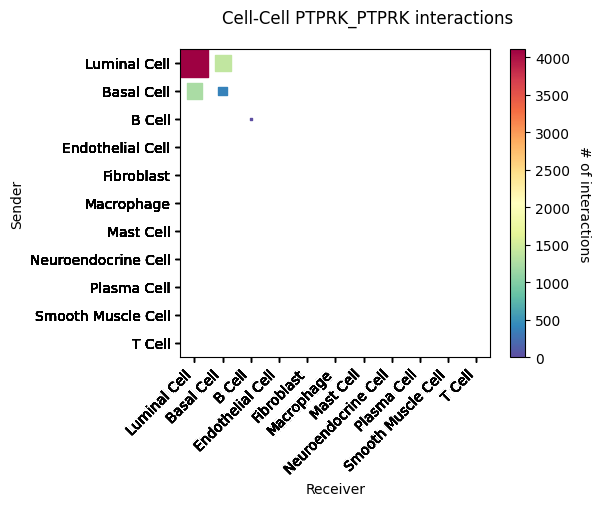
output

CCI heatmap shows cell type interactions. X and Y axes represent cell types; color represents interaction strength between two cell types.

Result Files

• lr_diagnostic_plots.png/pdf LR Diagnostic Plot

• lr_significant_scatter.png/pdf Significant Interacting LR Scatter Plot

• lr_significant_bar.png/pdf Significant Interacting LR Bar Plot

• celltype_lr_diagnostic_plots.png/pdf Cell Type LR Diagnostic Plot

• CCI_network_plots_*.png/pdf Cell Type Interaction Network Plot

• CCI_chord_plots_*.png/pdf Cell Type Interaction Chord Diagram

• *CCI_heatmap_plots.png/pdf Cell Type Interaction Heatmap

Literature Case Analysis

• Literature 1:
  The article "Spatially organized tumor-stroma boundary determines the efficacy of immunotherapy in colorectal cancer patients" used stlearn to reveal cell type interactions at the tumor-stroma boundary.

References

[1] Pham, D., Tan, X., Balderson, B. et al. Robust mapping of spatiotemporal trajectories and cell–cell interactions in healthy and diseased tissues. Nat Commun 14, 7739 (2023).

[2] Feng, Y., Ma, W., Zang, Y. et al. Spatially organized tumor-stroma boundary determines the efficacy of immunotherapy in colorectal cancer patients. Nat Commun 15, 10259 (2024).

Appendix

.xls, .txt: Result data table files, separated by tabs. Unix/Linux/Mac users use less or more commands to view; Windows users use advanced text editors like Notepad++ or Microsoft Excel.

.png: Result image files, bitmap, lossless compression.

.pdf: Result image files, vector graphics, scalable without distortion, convenient for viewing and editing, use Adobe Illustrator for editing, suitable for publication.