stLearn 空间转录组高级分析：受配体交互热点识别

作者: SeekGene

时长: 20 分钟

字数: 4.4k 字

更新: 2026-02-28

阅读: 0 次

空间转录组 分析指南 Notebooks 细胞通讯分析

背景介绍

stLearn 利用邻近位点间的配体（ligand）和受体（receptor）共表达信息以及细胞类型的多样性来计算配体-受体（LR）得分。并且能够在给定的组织内找到热点区域，在这些热点区域内，配受体相比于随机非交互基因对的空间分布，细胞类型间的 LR 交互更可能发生。（即考虑了邻近细胞间的通讯，以及受配体的共表达）

stlearn 的计算结果

import stlearn as st
import numpy as np
import pandas as pd
#matplotlib版本3.5.3，高版本的与stlearn有冲突
import matplotlib.pyplot as plt
import matplotlib.image as mpimg
import scanpy as sc
import re
import warnings
from PIL import Image
import os

output

/jp_envs/envs/stlearn/lib/python3.9/site-packages/stlearn/tools/microenv/cci/het.py:192: NumbaDeprecationWarning: The keyword argument 'nopython=False' was supplied. From Numba 0.59.0 the default is being changed to True and use of 'nopython=False' will raise a warning as the argument will have no effect. See https://numba.readthedocs.io/en/stable/reference/deprecation.html#deprecation-of-object-mode-fall-back-behaviour-when-using-jit for details.
@jit(parallel=True, nopython=False)

stLearn 细胞通讯模块输入参数介绍：

• SAMple_name：样本名
• meta_path：metadata 文件路径
• spot_diameter_fullres：细胞/spot 的大小，与分析步骤中的空间距离范围相关
• species：物种，该处只能填"human"或者"mouse"
• meta_celltype_colums_name：设置 adata 对象 obs 中细胞类型的列名

sample_name = "N1"
meta_path = "../../data/AY1748480899609/meta.tsv"
spot_diameter_fullres = 50
species = "human"
meta_celltype_colums_name = "CellAnnotation"

• 读取 SeekSpace 数据并进行标准化、降维、聚类（需要提前将 input.rds 转化成矩阵文件）

adata = sc.read_10x_mtx("./filtered_feature_bc_matrix/")
spatial = pd.read_csv('./filtered_feature_bc_matrix/cell_locations.tsv',sep="\t",index_col=0)
spatial = spatial.loc[:,("x","y")]
selected_rows = spatial.loc[spatial.index.isin(adata.obs_names)]
selected_rows.columns = ["imagecol","imagerow"]
selected_rows = selected_rows.reindex(adata.obs_names)
selected_rows = selected_rows*0.265385
a = st.create_stlearn(count=adata.to_df(),spatial=selected_rows,library_id=sample_name, scale=1,spot_diameter_fullres=spot_diameter_fullres)
a.layers["raw_count"] = a.X
# Preprocessing
st.pp.normalize_total(a)
st.pp.log1p(a)
# Keep raw data
a.raw = a
st.pp.scale(a)
st.em.run_pca(a,n_comps=50,random_state=0)
st.pp.neighbors(a,n_neighbors=25,use_rep='X_pca',random_state=0)
st.tl.clustering.louvain(a,random_state=0)
sc.tl.umap(a)

output

Normalization step is finished in adata.X
Log transformation step is finished in adata.X
Scale step is finished in adata.X
PCA is done! Generated in adata.obsm['X_pca'], adata.uns['pca'] and adata.varm['PCs']


/jp_envs/envs/stlearn/lib/python3.9/site-packages/tqdm/auto.py:21: TqdmWarning: IProgress not found. Please update jupyter and ipywidgets. See https://ipywidgets.readthedocs.io/en/stable/user_install.html
from .autonotebook import tqdm as notebook_tqdm
2025-08-28 17:39:53.325920: I tensorflow/core/platform/cpu_feature_guard.cc:193] This TensorFlow binary is optimized with oneAPI Deep Neural Network Library (oneDNN) to use the following CPU instructions in performance-critical operations: SSE4.1 SSE4.2 AVX AVX2 AVX512F AVX512_VNNI AVX512_BF16 AVX_VNNI AMX_TILE AMX_INT8 AMX_BF16 FMA
To enable them in other operations, rebuild TensorFlow with the appropriate compiler flags.
2025-08-28 17:39:55.109291: I tensorflow/core/util/port.cc:104] oneDNN custom operations are on. You may see slightly different numerical results due to floating-point round-off errors from different computation orders. To turn them off, set the environment variable \`TF_ENABLE_ONEDNN_OPTS=0\`.


Created k-Nearest-Neighbor graph in adata.uns['neighbors']
Applying Louvain cluster ...n Louvain cluster is done! The labels are stored in adata.obs['louvain']

将注释好的细胞类型添加到adata对象中

cluster_name = "celltype"
celltype = pd.read_csv(meta_path,index_col=0,sep = "\t")
celltype = celltype.loc[a.obs.index]
a.obs[cluster_name] = celltype[meta_celltype_colums_name]
a.obs[cluster_name] = a.obs[cluster_name].astype('category')

• 将空间切片划分为长为 n_，宽为 n_
  注：为了节省时间，将空间片子划分成 n×n 的格子(相当于 bin)，进行后续细胞通讯分析（grid_step=True）；若想以单细胞级别计算细胞通讯，这一步可不做运行（grid_step=False）

grid_step=False
if grid_step:
    #n_ = 125
    print(f'{n_grid} by {n_grid} has this many spots:\n', n_grid*n_grid)
    a = st.tl.cci.grid(a,n_row=n_grid, n_col=n_grid, use_label = cluster_name)
    print(a.shape)

• 加载受配体库，计算受配体表达的显著性

lrs = st.tl.cci.load_lrs(['connectomeDB2020_lit'], species=species)



st.tl.cci.run(a, lrs,
                  min_spots = 20, #Filter out any LR pairs with no scores for less than min_spots
                  distance=None, # None defaults to spot+immediate neighbours; distance=0 for within-spot mode
                  n_pairs=10000, # Number of random pairs to generate; low as example, recommend ~10,000
                  n_cpus=12, # Number of CPUs for parallel. If None, detects & use all available.
                  )

output

Calculating neighbours...n 112 spots with no neighbours, 14 median spot neighbours.
Spot neighbour indices stored in adata.obsm['spot_neighbours'] & adata.obsm['spot_neigh_bcs'].
Altogether 1483 valid L-R pairs


Generating backgrounds & testing each LR pair...: 1%|▏ [ time left: 2:49:41 ]

受配体表达显著性结果

lr_info = a.uns['lr_summary']

lr_info

	n_spots	n_spots_sig	n_spots_sig_pval
THBS1_LRP1	3185	1505	1870
PTPRK_PTPRK	2622	1471	2013
A2M_LRP1	3078	1412	1845
VEGFA_GPC1	3258	1260	1897
PTPRM_PTPRM	2731	1203	1669
...	...	...	...
FGF3_FGFRL1	27	12	24
GHRH_VIPR1	24	12	24
INHBC_ACVR2A	25	12	20
NPPC_NPR3	21	12	20
BMP10_BMPR1A	21	6	13

1483 rows × 3 columns

- 行：受配体对  
- 第一列 n_spot：未经过 pval 过滤受配体对互作的细胞/spot 数量（总）  
- 第二列 n_spots_sig：经过矫正后的 pval 过滤后的受配体对显著互作的细胞/spot 数量  
- 第三列 n_spots_sig_pval：根据设定的 pval 过滤后的受配体对互作的细胞/spot 数量

st.tl.cci.adj_pvals(a, correct_axis='spot',
                   pval_adj_cutoff=0.05, adj_method='fdr_bh')

output

Updated adata.uns[lr_summary]
Updated adata.obsm[lr_scores]
Updated adata.obsm[lr_sig_scores]
Updated adata.obsm[p_vals]
Updated adata.obsm[p_adjs]
Updated adata.obsm[-log10(p_adjs)]

受配体诊断图

受配体分析的一个关键方面是在确定显著 hotspot 时，控制受配体的表达水平和频率。因此，诊断图应显示受配体对的热点与表达水平和表达频率之间几乎没有相关性。以下诊断方法可以帮助检查和确认这一点；如果不是这样，表明可能需要更大数量的 Permutations。

st.pl.lr_diagnostics(a, show=False,figsize=(15,5))

output

(Figure size 1500x500 with 2 Axes,
array([,
],
dtype=object))

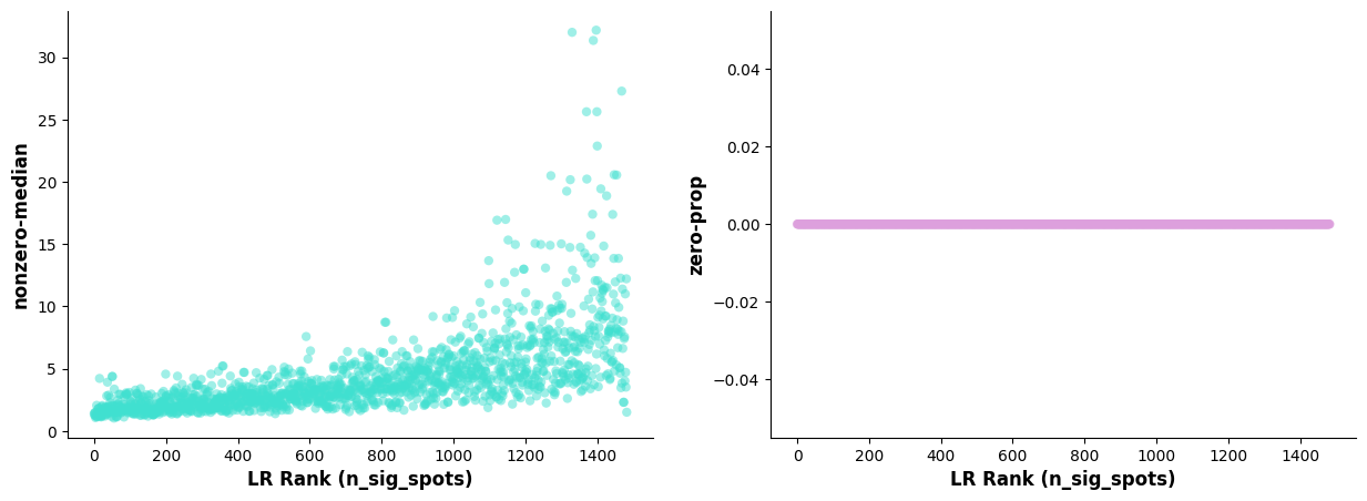
* **左图：** 横轴为 n_spots_sig 的排序受配体对;纵轴为受配体对(非零)表达中位值。
* **右图：** 横轴为 n_spots_sig 的排序受配体对；纵轴为受配体对表达值为 0 的细胞占所有细胞的比例。

显著互作的受配体散点图

#st.pl.lr_summary(a, n_top=500,show=False)
st.pl.lr_summary(a, n_top=50, show=False,figsize=(10,3))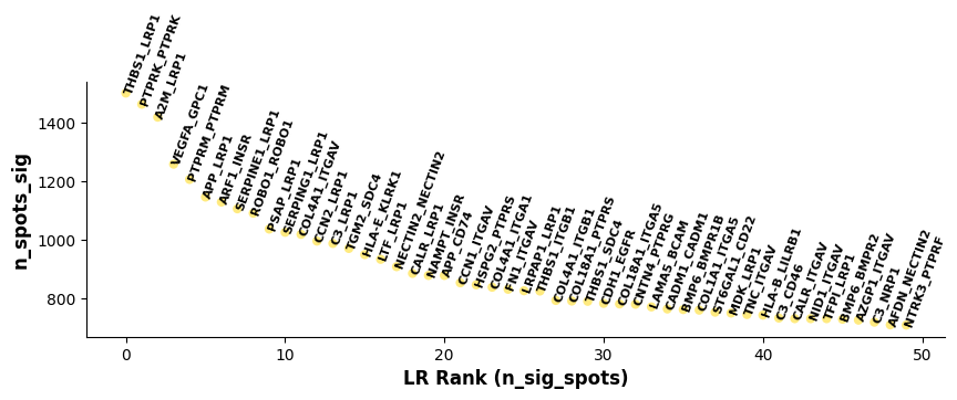

output

基于 lr_summary 的结果作图：展示了 top50 的受配体对。横轴代表 n_spots_sig 的排序受配体对；纵轴代表经 pval 过滤矫正后的受配体对显著互作的细胞/spot 数量。

显著互作的受配体柱状图

st.pl.lr_n_spots(a, n_top=50,max_text=100,show=False,figsize=(11, 3))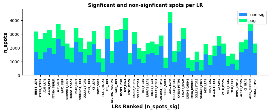

output

(Figure size 1100x300 with 1 Axes,
)

基于 lr_summary 的结果作图：展示了 top500 和 top50 的受配体对。横轴代表 n_spots_sig 的排序受配体对；纵轴代表未经过 pval 过滤受配体对互作的细胞/spot 数量（总）；绿色和蓝色分别代表显著和不显著受配体对。

LR 统计学可视化

可视化显著受配体对共表达的热点区域，可以大致看出感兴趣的受配体对发生互作集中的区域

lr_scores = pd.DataFrame(a.obsm["lr_scores"])
lr_scores.columns = lr_info.index
lr_scores.index = a.obs.index

p_vals = pd.DataFrame(a.obsm["p_vals"])
p_vals.columns = lr_info.index
p_vals.index = a.obs.index

p_adjs = pd.DataFrame(a.obsm["p_adjs"])
p_adjs.columns = lr_info.index
p_adjs.index = a.obs.index

log10_p_adjs = pd.DataFrame(a.obsm["-log10(p_adjs)"])
log10_p_adjs.columns = lr_info.index
log10_p_adjs.index = a.obs.index

spatial["LR_score"] = list(lr_scores["THBS1_LRP1"])
spatial["p_vals"] = list(p_vals["THBS1_LRP1"])
spatial["p_adjs"] = list(p_adjs["THBS1_LRP1"])
spatial["-log10(p_adjs)"] = list(log10_p_adjs["THBS1_LRP1"])

spatial

	x	y	LR_score	p_vals	p_adjs	-log10(p_adjs)
Barcode
AACCTGAGCTAGATTAGAGCGACGGAT_1	16898	9879	0.000000	1.0000	1.00000	-0.000000
AAGACAAGCTGATACCTGCTCTGCTTC_1	40296	7851	1.194025	0.0111	0.01353	1.868702
AAGTACCCGAGATAAACAAGGCACTAT_1	31685	6429	-0.203235	1.0000	1.00000	-0.000000
AGAAGCGGCTTCCGATACCTAATAACG_1	16767	17485	-0.460579	1.0000	1.00000	-0.000000
AGACTCAATGAATGCACTTCTGCGCTC_1	11746	14166	-0.203235	1.0000	1.00000	-0.000000
...	...	...	...	...	...	...
TCCGATCCGAAGGAGGGAAGGCACTAT_1	30882	9777	-0.314717	1.0000	1.00000	-0.000000
TGAGGAGGCTCGACAAGTTCTGCGCTC_1	45879	10249	-0.004137	1.0000	1.00000	-0.000000
AGGTCTACGATGTGGAGGCTCTGCTTC_1	54295	6672	0.000000	1.0000	1.00000	-0.000000
TTCCTTCATGCGCTTCGAAGGCACTAT_1	30565	10833	0.000000	1.0000	1.00000	-0.000000
CATAAGCGCTACTCAACGGACTGTGGA_1	16847	944	-0.196527	1.0000	1.00000	-0.000000

20820 rows × 6 columns

# 读取空间HE或者DAPI
background_image = mpimg.imread('filtered_feature_bc_matrix/N1_expression.png')

# 创建一个新的图形
fig, ax = plt.subplots(figsize=(12, 8))

# 显示底片图像
ax.imshow(background_image, extent=[0, 55050, 0, 19906], aspect='auto')

# 选择用于颜色渐变的数值列（请根据您的数据修改列名）
# 例如：'expression_level', 'score', 'intensity' 等
value_column = 'LR_score'  # 请替换为实际的数值列名

# 创建颜色映射
# 可以选择不同的colormap：'viridis', 'plasma', 'inferno', 'magma', 'coolwarm', 'RdBu_r' 等
cmap = plt.cm.viridis
norm = plt.Normalize(vmin=spatial[value_column].min(), 
                    vmax=spatial[value_column].max())

# 创建散点图，根据数值列设置颜色
scatter = ax.scatter(spatial['x'], spatial['y'], 
                    c=spatial[value_column], 
                    cmap=cmap, norm=norm, 
                    alpha=0.7, s=15, edgecolors='none')

# 添加颜色条
cbar = plt.colorbar(scatter, ax=ax, shrink=0.8)
cbar.set_label(value_column, fontsize=12)

# 添加标签和标题
ax.set_xlabel('Spatial_1', fontsize=12)
ax.set_ylabel('Spatial_2', fontsize=12)
ax.set_title(f'THBS1_LRP1 {value_column}', fontsize=14)

# 移除坐标轴刻度（可选，使图片更美观）
ax.set_xticks([])
ax.set_yticks([])
ax.set_aspect("equal")
# 显示图形
plt.tight_layout()
plt.show()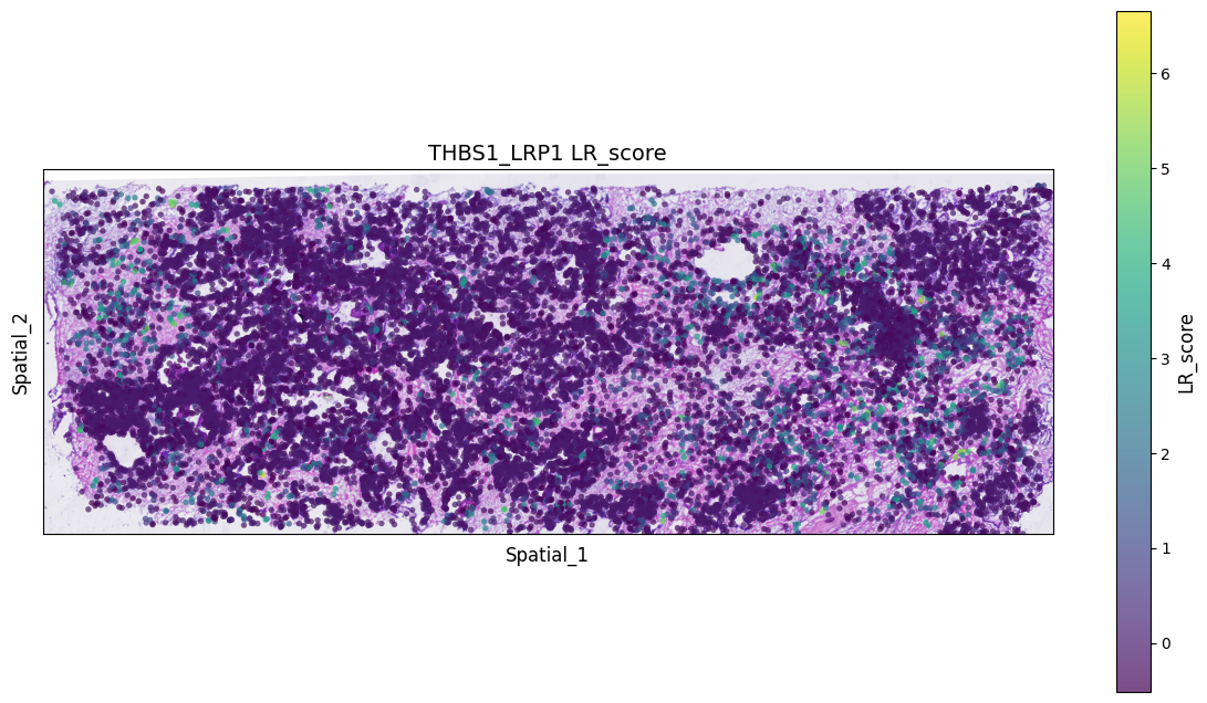

# 读取空间HE或者DAPI
background_image = mpimg.imread('filtered_feature_bc_matrix/N1_expression.png')

# 创建一个新的图形
fig, ax = plt.subplots(figsize=(12, 8))

# 显示底片图像
ax.imshow(background_image, extent=[0, 55050, 0, 19906], aspect='auto')

# 选择用于颜色渐变的数值列（请根据您的数据修改列名）
# 例如：'expression_level', 'score', 'intensity' 等
value_column = 'p_adjs'  # 请替换为实际的数值列名

# 创建颜色映射
# 可以选择不同的colormap：'viridis', 'plasma', 'inferno', 'magma', 'coolwarm', 'RdBu_r' 等
cmap = plt.cm.viridis
norm = plt.Normalize(vmin=spatial[value_column].min(), 
                    vmax=spatial[value_column].max())

# 创建散点图，根据数值列设置颜色
scatter = ax.scatter(spatial['x'], spatial['y'], 
                    c=spatial[value_column], 
                    cmap=cmap, norm=norm, 
                    alpha=0.7, s=15, edgecolors='none')

# 添加颜色条
cbar = plt.colorbar(scatter, ax=ax, shrink=0.8)
cbar.set_label(value_column, fontsize=12)

# 添加标签和标题
ax.set_xlabel('Spatial_1', fontsize=12)
ax.set_ylabel('Spatial_2', fontsize=12)
ax.set_title(f'THBS1_LRP1 {value_column}', fontsize=14)

# 移除坐标轴刻度（可选，使图片更美观）
ax.set_xticks([])
ax.set_yticks([])
ax.set_aspect("equal")
# 显示图形
plt.tight_layout()
plt.show()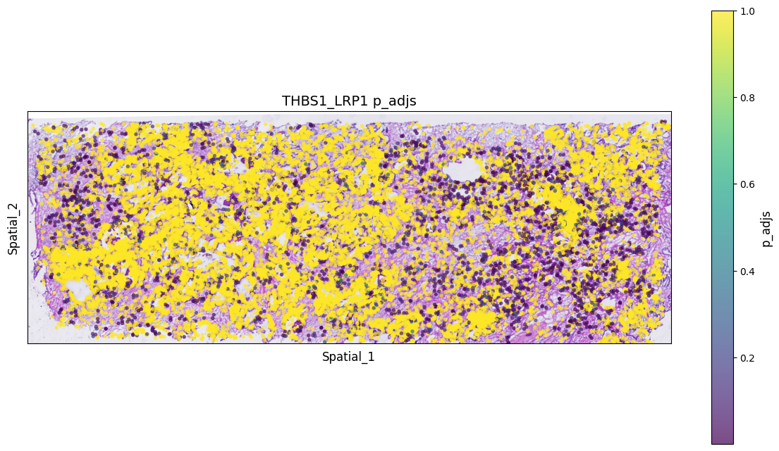

• 预测显著互作的细胞类型

st.tl.cci.run_cci(a, cluster_name, # Spot cell information either in data.obs or data.uns
                  min_spots=3, # Minimum number of spots for LR to be tested.
                  sig_spots=True, # Only consider neighbourhoods of spots which had significant LR scores.
                  n_perms=1000, # Permutations of cell information to get background, recommend ~1000
                  n_cpus=16
                 )

output

Getting cached neighbourhood information...n Getting information for CCI counting...n

Counting celltype-celltype interactions per LR and permutating 1000 times.: 0%| [ time left: 31:03:47 ]

细胞类型诊断图

检查受配体互作和细胞类型的细胞数之间的相关性，如果 permutations 的数量足够，下面的图表应该显示几乎没有或没有相关性；否则，建议将 n_perms（置换次数）的值调高。

st.pl.cci_check(a, cluster_name,show=False,figsize=(10,4),cell_label_size=10,axis_text_size=12)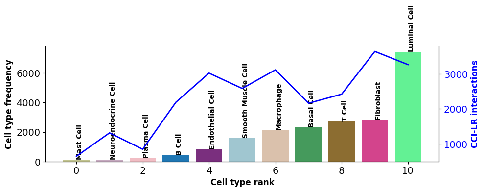

output

(Figure size 1000x400 with 2 Axes,
,
)

横轴代表细胞类型；柱状图对应的左纵轴代表细胞类型数量；折线对应的由纵轴代表细胞类型互作的受配体数量。

CCI 网络图

st.pl.ccinet_plot(a, cluster_name, return_pos=True,pad=0.3,node_size_exp=0.8)


lr_pair = a.uns['lr_summary'].index.values[0:3]
st.pl.ccinet_plot(a, cluster_name, lr_pair[1], min_counts=2,pad=0.3,node_size_exp=0.8)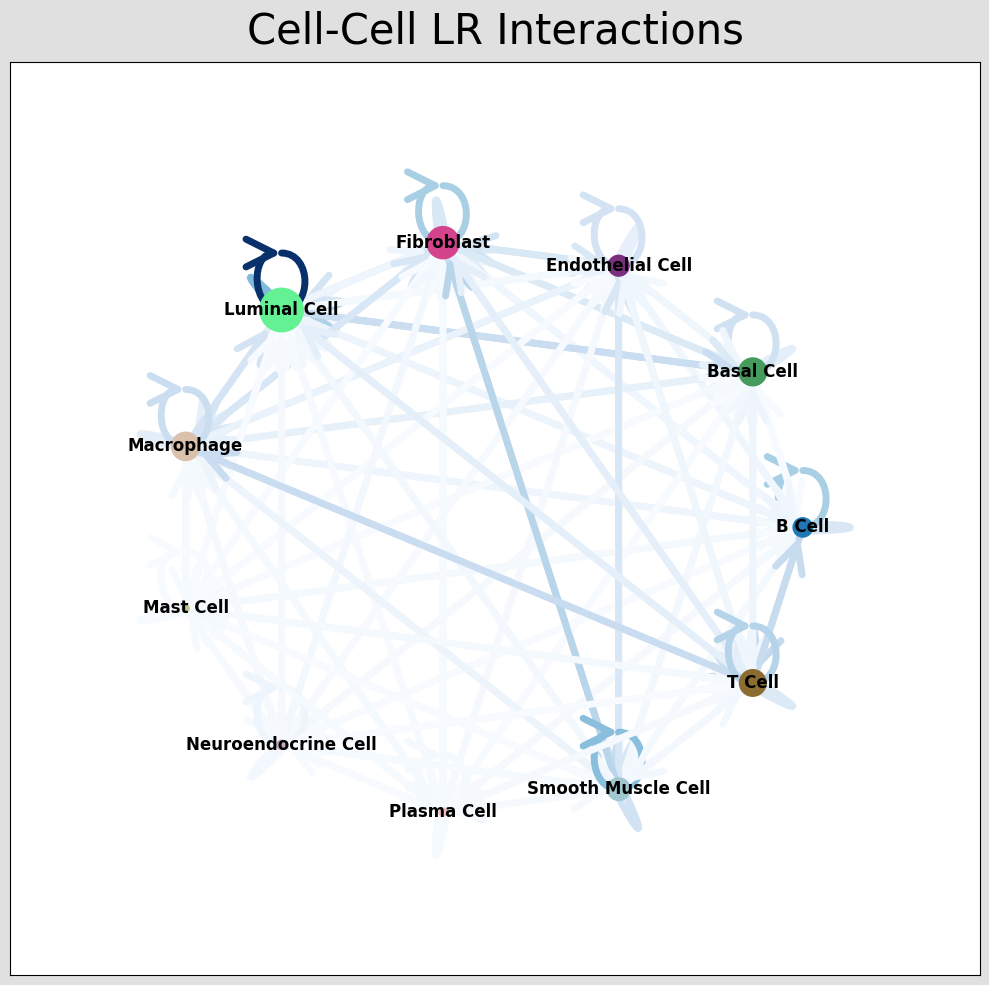

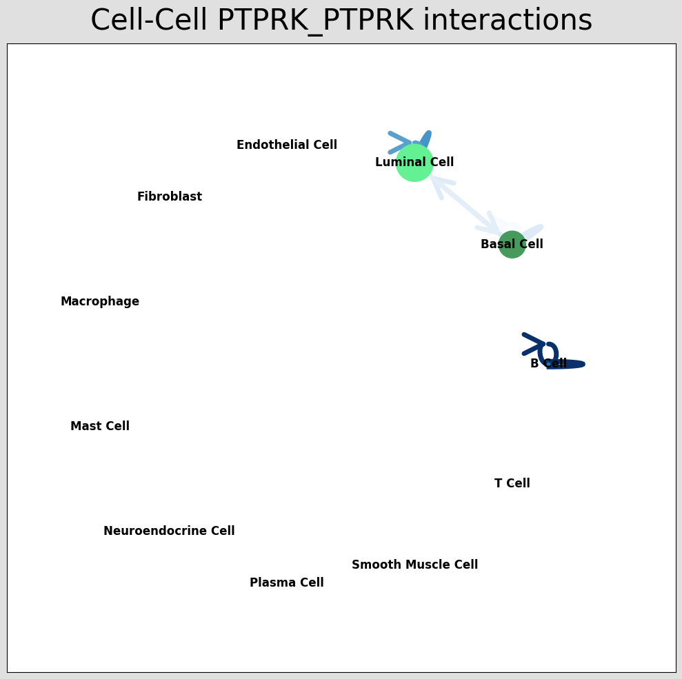
细胞通讯网络图中展示对应受配体对的细胞类型互作情况，通过结果 per_lr_cci_*绘制的。每一种颜色代表着一种细胞类型；线条从一个细胞类型指向自己或者其他的细胞类型，代表着互作的情况；线条颜色的深浅代表着细胞类型之间互作的强度。

CCI 和弦图

st.pl.lr_chord_plot(a, cluster_name,show=False)


st.pl.lr_chord_plot(a, cluster_name,show=False,lr=lr_pair[1])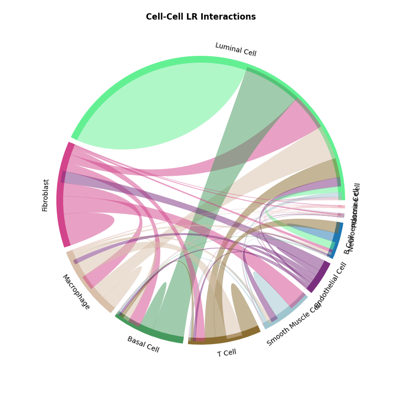

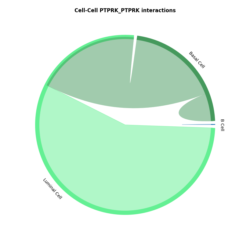
output

(Figure size 800x800 with 1 Axes, Axes:)

细胞通讯和弦图中展示对应受配体对的细胞类型互作情况，通过结果 per_lr_cci_*绘制的。每一种颜色代表着一种细胞类型；弦的宽度表示细胞间相互作用的强度，较宽的弦表示较强的相互作用，较窄的弦表示较弱的相互作用。

CCI 热图

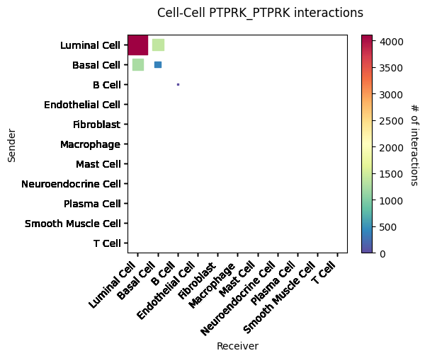
st.pl.lr_cci_map(a, cluster_name, lrs=None, min_total=100, figsize=(20,4),show=False)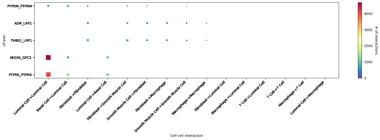

output

细胞通讯热图中展示细胞类型对应的受配体互作情况。横轴代表互作的细胞类型；纵轴代表互作的受配体；颜色代表着互作强度，颜色越红，互作越强。展示了 top5 显著互作较强的受配体对

st.pl.cci_map(a, cluster_name,show=False,figsize=(5,4))


st.pl.cci_map(a, cluster_name, lr=lr_pair[1],show=False,figsize=(5,4))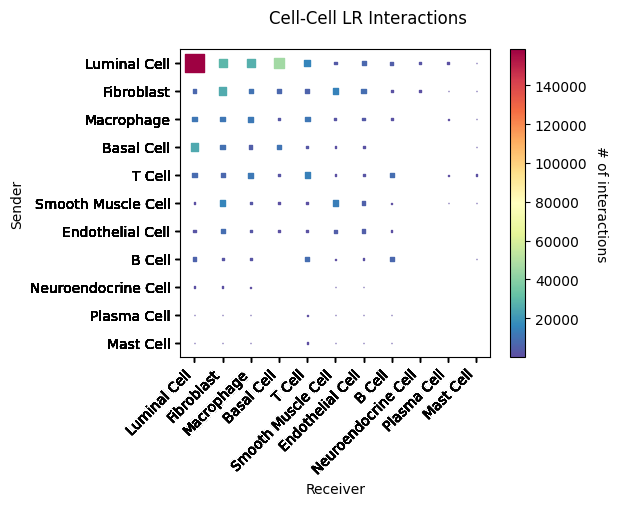

output

细胞通讯热图中展示细胞类型的互作情况。横轴和纵轴代表着细胞类型；颜色代表着两个细胞类型互作强度。

结果文件

• lr_diagnostic_plots.png/pdf 受配体诊断图

• lr_significant_scatter.png/pdf 显著互作的受配体散点图

• lr_significant_bar.png/pdf 显著互作的受配体柱状图

• celltype_lr_diagnostic_plots.png/pdf 细胞类型受配体诊断图

• CCI_network_plots_*.png/pdf 细胞类型互作网络图

• CCI_chord_plots_*.png/pdf 细胞类型互作和弦图

• *CCI_heatmap_plots.png/pdf 细胞类型互作热图

文献案例解析

• 文献一：
  文献《Spatially organized tumor-stroma boundary determines the efficacy of immunotherapy in colorectal cancer patients》使用 stlearn 去揭示肿瘤与基质区的交界处的细胞类型互作情况。

参考文献

[1] Pham, D., Tan, X., Balderson, B. et al. Robust mapping of spatiotemporal trajectories and cell–cell interactions in healthy and diseased tissues. Nat Commun 14, 7739 (2023).
[2] Feng, Y., Ma, W., Zang, Y. et al. Spatially organized tumor-stroma boundary determines the efficacy of immunotherapy in colorectal cancer patients. Nat Commun 15, 10259 (2024).

附录

.xls,.txt ：结果数据表格文件，文件以制表符（Tab）分隔。unix/Linux/Mac 用户使用 less 或 more 命令查看；windows 用户使用高级文本编辑器 Notepad++ 等查看，也可以用 Microsoft Excel 打开。

.png：结果图像文件，位图，无损压缩。

.pdf：结果图像文件，矢量图，可以放大和缩小而不失真，方便用户查看和编辑处理，可使用 Adobe Illustrator 进行图片编辑，用于文章发表等。