Banksy spatial clustering principles installation code examples and interpretation
Introduction
NOTE
This document introduces the principles, installation, usage, and result interpretation of the Banksy (BANKSY) spatial clustering R package, suitable for cell type identification and spatial domain segmentation in single-cell spatial transcriptomics data.
Principle Overview
IMPORTANT
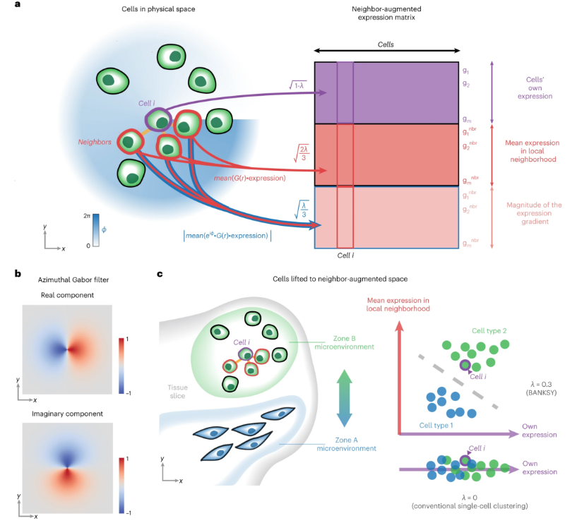
Banksy is a spatial omics clustering method that enhances each cell's feature vector by integrating the mean expression of its spatial neighbors and spatial gradient features, thereby improving clustering. This approach can:
- Improve cell type assignment in noisy data.
- Distinguish subtle cell subtypes influenced by the microenvironment.
- Identify spatial domains with similar microenvironments.
Banksy is applicable to various spatial transcriptomics technologies (e.g., SeekSpace, Slide-seq, MERFISH, CosMX, etc.) and is scalable to large datasets.
Data Preparation
Example Data
The official Banksy R package provides mouse hippocampus spatial transcriptomics data for direct testing.
# Load example data
library(Banksy)
data(hippocampus)
gcm <- hippocampus$expression
locs <- as.matrix(hippocampus$locations)
User Data
- Expression matrix (genes × cells/spots).
- Spatial coordinates matrix (cells/spots × 2).
Environment Installation
IMPORTANT
Requires R >= 4.4.0. Bioconductor installation is recommended.
# Install via Bioconductor
if (!requireNamespace("BiocManager", quietly = TRUE))
    install.packages("BiocManager")
BiocManager::install('Banksy')

# Or install the latest version from GitHub
if (!requireNamespace("remotes", quietly = TRUE))
    install.packages("remotes")
remotes::install_github("prabhakarlab/Banksy")
TIP
It is recommended to also install SpatialExperiment, scuttle, scater, ggplot2, and cowplot for data processing and visualization.
BiocManager::install(c("SpatialExperiment", "scuttle", "scater"))
install.packages(c("ggplot2", "cowplot"))
Example Workflow
# Load required packages
library(Banksy)
library(SpatialExperiment)
library(scuttle)
library(scater)
library(ggplot2)
library(cowplot)

# Construct SpatialExperiment object
se <- SpatialExperiment(assay = list(counts = gcm), spatialCoords = locs)

# Quality control and normalization
qcstats <- perCellQCMetrics(se)
thres <- quantile(qcstats$total, c(0.05, 0.98))
keep <- (qcstats$total > thres[1]) & (qcstats$total < thres[2])
se <- se[, keep]
se <- computeLibraryFactors(se)
assay(se, "normcounts") <- normalizeCounts(se, log = FALSE)

# Compute Banksy neighborhood features
lambda <- c(0, 0.2)
k_geom <- c(15, 30)
se <- Banksy::computeBanksy(se, assay_name = "normcounts", compute_agf = TRUE, k_geom = k_geom)

# Dimensionality reduction and clustering
set.seed(1000)
se <- Banksy::runBanksyPCA(se, use_agf = TRUE, lambda = lambda)
se <- Banksy::runBanksyUMAP(se, use_agf = TRUE, lambda = lambda)
se <- Banksy::clusterBanksy(se, use_agf = TRUE, lambda = lambda, resolution = 1.2)
se <- Banksy::connectClusters(se)

# Visualization
cnames <- colnames(colData(se))
cnames <- cnames[grep("^clust", cnames)]
colData(se) <- cbind(colData(se), spatialCoords(se))
plot_nsp <- plotColData(se, x = "sdimx", y = "sdimy", point_size = 0.6, colour_by = cnames[1])
plot_bank <- plotColData(se, x = "sdimx", y = "sdimy", point_size = 0.6, colour_by = cnames[2])
plot_grid(plot_nsp + coord_equal(), plot_bank + coord_equal(), ncol = 2)
Parameter Description
| Parameter | Description |
|---|---|
| lambda | Weight of spatial neighborhood features; 0 for non-spatial, 0.2 recommended for cell typing. |
| k_geom | Number of spatial neighbors, recommended 15 and 30. |
| use_agf | Whether to use neighborhood mean and gradient features. |
| resolution | Clustering resolution, affects the number of clusters. |
| assay_name | Name of the expression matrix used (e.g., normcounts). |
WARNING
- The recommended lambda value may differ for datasets with different spatial resolutions; see the official documentation for details.
- For large datasets, high-performance computing resources are recommended.
Main Results Interpretation
- Clustering labels: The clust_* columns in colData(se) correspond to clustering results under different lambda values.
- Dimensionality reduction: UMAP and other coordinates are stored in reducedDims(se).
- Visualization: Use plotColData, plotReducedDim, etc., to visualize spatial clustering.
NOTE
Banksy clustering results can be used for downstream spatial subtype analysis, domain identification, microenvironment studies, etc.